Reliability theory in operational research

A Thesis Submitted for the Degree of PhD

at the

University of St Andrews

1991

Full metadata for this item is available in

St Andrews Research Repository

at:

http://research-repository.st-andrews.ac.uk/

Please use this identifier to cite or link to this item:

http://hdl.handle.net/10023/13745

FADIL AJAB AL-BAIDHANI

A thesis submitted for the Degree of Doctor of Philosophy at the University of St. Andrews

Department of Mathematical and Computational Sciences Division of Statistics

INFORMATION TO ALL USERS

The quality of this reproduction is dependent upon the quality of the copy submitted.

In the unlikely event that the author did not send a com plete manuscript and there are missing pages, these will be noted. Also, if material had to be removed,

a note will indicate the deletion.

uest

ProQuest 10167343

Published by ProQuest LLO (2017). Copyright of the Dissertation is held by the Author.

All rights reserved.

This work is protected against unauthorized copying under Title 17, United States C ode Microform Edition © ProQuest LLO.

ProQuest LLO.

789 East Eisenhower Parkway P.Q. Box 1346

my wife Selma my children, Mohammed, Inas, and Mohanned

and

to the memory of my mother

Signed ( F. A. Al-Baidhani ) Dated:

Signed ( F. A. Al-Baidhani ) Dated:

Signature of Supervisor ( C. D. Sinclair ) Dated:

I Fadil Ajab Naher Al- Baidhani hereby certify that this thesis has been composed by myself, that it is a record of my own work, and that it has not been accepted in partial or com plete fulfilm ent of any other degree of* professional q u a lifica tio n .

DECLARATION

I was admitted to the Faculty of Science of the University of St Andrews under Ordinance General No. 12 in January 1986, and

as a candidate for the degree of Ph. D. in October 1986.

I

DECLARATION

Special gratitude is due to Prof. R. M, Cormack who made it possible for me to pursue my research at the University of St Andrews.

No words can express the gratitude felt to my wife, Selma, for her support, encouragement and patience.

Finally I am indebted to the Government of the Republic of Iraq for financial support.

understand that I am giving permission for it to be made

I

University Library for the time being in force, subject to any copyright vested In the work being affected thereby. I also understand that the title and abstract will be published, and that a copy of the work may be made and supplied to any bona fide library or research worker.

ACKNOWLEDGEMENTS

Without the incessant guidance and help of my supervisor Mr.

0. D. Sinclair this work would not have been possible. I am

extremely grateful to him for his continuous encouragement ^ throughout the course of this study.

estimating the parameters of the Weibull and Beta distributions using several different techniques. These distributions are used

in the area of reliability testing and it is important to achieve v-the best estimates possible of v-the parameters involved. After

considering several accepted methods of estim ating the relevant parameters, it is considered that the best method depends on the aim of the analysis, and on the value of the shape param eter p. For estimating the two-param eter Weibull distribution, it is recommended that Generalized Least Squares (GLS) is the best method to use for values of p between 0.5 and 30. However, Maximum Likelihood Estimator (MLE) is a good method for estimating quantiles.

On this basis, the three-parameter Weibull distribution is Investigated. The traditional parametrization is compared with a new parametrization developed in this work. By considering parameter effects and intrinsic curvature it is shown that the new parametrization results in a linear effect of the shape parameter. Also it has advantages in quantile estimation because of its ability to provide estimates for a wider range of data sets.

DECLARATIONS

ACKNOWLEDGEMENTS

ABSTRACT

LIST OF TABLES

LIST OF FIGURES

LIST OF PLATES

NOTATION

CHAPTER 1 1

1.1 INTRODUCTION 1

1.2 ESTIMATION 4

1.3 THE STRUCTURE OF THE THESIS 6

PARAMETERS OF THE WEIBULL DISTRIBUTION

2.1 INTRODUCTION 11

2.2 THE METHODS 14

2.3 EXAMPLES 22

2.4 SIMULATION 36

2.5 SUMMARY AND CONCLUSION 62

CHAPTER 3 63

A NEW PARAMETRIZATION AND GENERALIZATION OF THE THREE-PARAMETER WEIBULL

DISTRIBUTION

3.1 INTRODUCTION 64

3.2 A NEW PARAMETRIZATION AND GENERALIZATION OF THE

THREE-PARAMETER WEIBULL DISTRIBUTION 70

3.3 COMPARISON BETWEEN THE ORDINARY WEIBULL DISTRIBUTION AND THE NEW PARAMETRIZATION

(K > 0) 74

'3

■I

3.6 SIMULATION 104

3.7 SUMMARY AND CONCLUSIONS 112

CHAPTER 4 114

ESTIMATION OF PARAMETERS OF THE BETA DISTRIBUTION

4.1 INTRODUCTION 115

4.2 METHODS FOR THE TWO PARAMETERS CASE 11 8

4.3 METHODS FOR THE FOUR PARAMETERS CASE 1 2 0

4.4 EXAMPLE 134

4.5 SIMULATION 140

4.6 SUMMARY AND CONCLUSIONS 18 0

FOR FURTHER RESEARCH

5.1 INTRODUCTION 184

5.2 POINT ESTIMATION FOR THE TWO-PARAMETER

WEIBULL DISTRIBUTION 1 85

5.3 USE OF GW DISTRIBUTION 18 7

5.4 POINT ESTIMATION FOR THE FOUR-PARAMETER BETA

DISTRIBUTION 189 |

5.5 ASYMPTOTIC DISTRIBUTION OF ESTIMATORS 1 92

5.6 APPLICATION TO CERAMICS 193

5.7 FINAL REMARKS 193

REFERENCES 194

2.1b Estimated values of parameters for sample number 2

using various methods. 23

2.2 Summary of the results of various methods. 24

2.3a GLS for the two-parameter Weibull distribution, and Anderson-Darling test statistic values. 26

2.3b MLE for the two-parameter Weibull distribution, and Anderson-Darling test statistic values. 27

2.4 Observed relative efficiencies for estimators of

Weibull parameters p and a (n=25). 41

2.5 Average relative efficiency of each estimator across

param etrizations. 42

2.6 Monte Carlo simulation of the Weibull parameters based on 1000 random samples, with sample size n, shape parameter p, scale parameter a, standar

deviation (SD), bias, and root mean square error (RMSE)

for both parameters. 45'

2.7 Estimated variance of a and p when a =1. 46

3.1 Some properties of the GW distribution. 72

3.2 Incremental values of k, p and their values of skewness

and kurtosis. 76

3.3 Illustrative data set. 79

3.4a MLE of the two-parameter Weibull distribution,

Anderson-Darling test statistic values, and 1% critical

value of A^. 100

3.4b PWM of the three-parameter Weibull distribution, Anderson-Darling test statistic values, and the

coefficient of skewness. 100

3.4c PWM of the GW distribution (case k > 0), Anderson-Darling test statistic values, and 5% critical value

of A^. 101

3.5 Estimated values of the parameters of the GW

distribution, the Anderson-Darling test statistic value,

and the coefficient of skewness. 102

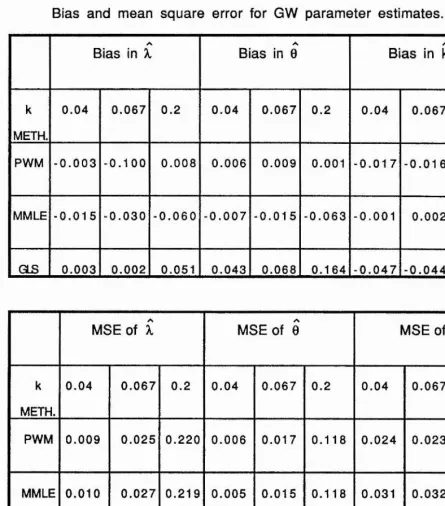
3.6 Bias and mean square error for GW parameter

estim ates. 106

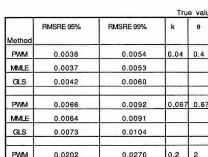
3.7 Root mean squared relative error of the predicted quantiles for data sets where MMLE found

MMLE. 11 0

3.10 Root mean squared relative error of the predicted quantiles for data sets that give positive k

estim ate. 111

4.1a Regression equations to obtain smooth values of correlation coefficient for estimating the parameter

a. 127

4.1b Regression equation to obtain smooth values of

correlation coefficient for estimating the parameter

c. 127

4.2 Deviance for the fit of the numbers of observed

correlation coefficients that lie below the smoothed

critical values 129

4.3 Estimated values of the parameters of Beta

distribution, and the values of the Anderson-Darling

test statistic. 135

4.4a Result of 200 simulations with q=10 used to

compare four methods of estimation through the RMSE, bias, and variance for estimators a, c, p, and q. 143

4.4b Result of 200 simulations with q=3 used to compare

■4i

4.5a Result of 74 simulations with q=10 used to compare four methods of estimation through the RMSE, bias, and variance for estimators a, c, p, and q. 145

4.5b Result of 129 simulations with q«3 used to compare four methods of estimation through the RMSE, bias, and

variance for estimators a, c, p, and q. 146 I

4.6 Comparison of methods using Bias, Variance, and RMSE

of 5% and 95% quantiles when (p, q) are (2, 3) for 200 f

data sets. 149

i

4.7 Comparison of methods using Bias, Variance, and RMSE

of 5% and 95% quantiles when (p, q) are (2, 3) for 129 | data sets for which the ME is feasible. 1 50

4.8 Comparison of methods using Bias, Variance, and RMSE ^

J

data sets. 151

4.9 Comparison of methods using Bias, Variance, and RMSE | of 5% and 95% quantiles when (p, q) are (2, 10) for 74

GLS. 28

2.1b Cdf and Edf of the ceramic data of size 50 of the

two-parameter Weibull distribution fitted by GLS. 29 I

2.1c Histogram of the ceramic data of size 50 and pdf of the two-parameter Weibull distribution fitted by

MLE. 30

2.1 d Cdf and Edf of the ceramic data of size 50 of the two-parameter Weibull distribution fitted by MLE. 31

2.2a Histogram of the ceramic data of size 45 and pdf of the two-parameter Weibull distribution fitted by

GLS. 32

2.2b Cdf and Edf of the ceramic data of size 45 of the

two-parameter Weibull distribution fitted by GLS. 33

2.2c Histogram of the ceramic data of size 45 and pdf of

1

MLE. 34

2.2d Cdf and Edf of the ceramic data of size 45 of the

two-parameter Weibull distribution fitted by MLE. 35

2.3 Empirical efficiency of estimates of shape parameter by various methods, from simulated sample of

size 10. 51

-i'-2.4 Empirical efficiency of estimates of shape parameter by various methods, from simulated sample of

size 25. 52

2.5 Empirical efficiency of estimates of scale parameter by various methods, from simulated sample of size

10. 54

2.6 Empirical efficiency of estimates of scale parameter by various methods, from simulated sample of size

25. 55

2.7 The root mean square relative error of estimates of the 95% percent quantile with parameters estimated by various methods from simulated sample of size 10. 57

2.8 The root mean square relative error of estimates of the 95% percent quantile with parameters estimated by various methods from simulated sample of

size 25. 58

2.9 The root mean square relative error of estimates of the 99% percent quantile with parameters estimated by various methods from simulated sample of size 10. 59

2.11 Variability of RE for shape and scale parameters using

GLS. 61

■I

2.10 The root mean square relative error of estimates of the 99% percent quantile with parameters estimated by

various methods from simulated sample of size 25. 60 f

I

3.2a Pdf of Weibull distribution with different values of p

and same a=1. 68

3.2b Pdf of Weibull distribution with different values of p, same mean and standard deviation (i.e standarised

version). 69

3.3 Hazard functions for GW with k > 0 and k < 0. 73

3.4 The relation between skewness and shape parameter

k for the GW distribution. 74

3.5 Points corresponding to equal increments in k for GW parametrization of Weibull distribution. 77

3.6 Points corresponding to equal increments in p for the

ordinary Weibull distribution. 78

3.7 Sample space representation of data

(equation 3.3.1). 82

3.8 Sample space representation of data

(equation 3.3.2). 83

3.9 The profile likelihood for Smith's sample 1 with his

param etrization, 85

3.10 The profile likelihood for the Smith's sample 1 with

3.11a Cdf for the two- and three-parameter Weibull

distributions with Edf of the Ceramic data set of size

26. 98

3.11b Cdf for the two- and three-parameter Weibull

distributions with Edf of the Ceramic data set of size

32. 99

3.12 Histogram of the fiber data and pdf of the GW

distribution. 103

4.1a Quantile-quantile plot of the theoretical quantiles for sample number 25 with q=10 against the ordered data, illustrating an upper outlier. 131

4.1b Probability-plot of the sample number 106 with q=10 against four parameter Beta distribution,

illustrating lower outliers. 132

4.2a Probability-plot of the Caterpillar Right Rear Brake data against the three parameter Beta distribution. 138

4.2b Probability-plot of the Caterpillar Right Rear Brake data against the two parameter Weibull

distribu tion . 139

4.3 Histogram of estimated values obtained by MMLE of (a) 5% and (b) 95% quantiles with q=3. 155

4.6 4.7 4.8 4.9 4.10 4.11 4.12 4.13

Histogram o (a) 5% and

Histogram o (a) 5% and

Histogram o (a) 5% and

Histogram o (a) 5% and

Histogram o (a) 5% and

Histogram o (a) 5% and

Histogram o

estimated values obtained by SMLE of b) 95% quantiles with q-3. 158

estimated values obtained by ME of b) 95% quantiles with q=3. 159

estimated values obtained by MMLE of (b) 95% quantiles with q=10. 160

estimated values obtained by CORBPE of b) 95% quantiles with q=10. 161

estimated values obtained by SMLE of b) 95% quantiles with q=10. 162

estimated values obtained by SME of b) 95% quantiles with q=10. 163

estimated values obtained by ME of

(a) 5% and (b) 95% quantiles with q=10. 164

Plot of the square root of A and -LL vs number of observations. The estimated values are obtained by

4.15 Plot of the square root of A^ and -LL vs number of observations. The estimated values are obtained by

SMLE with q=3. 169

4.16 Plot of the square root of P ? and -LL vs number of observations. The estimated values are obtained by

SME with q=3. 170

4.17 Plot of the square root of A^ and -LL vs number of observations. The estimated values are obtained by

ME with q=3. 171

p

4.18 Plot of the square root of A and -LL vs number of observations. The estimated values are obtained by

MMLE with q=10. 172

4.19 Plot of the square root of A^ and -LL vs number of observations. The estimated values are obtained by

CORBPE with q=10. 173

4.20 Plot of the square root of A^ and -LL vs number of observations. The estimated values are obtained by

SMLE with q=10. 174

p

4.21 Plot of the square root of A and -LL vs number of observations. The estimated values are obtained by

4.23

4.24

Trimmed mean of the - log likelihood with q=1 0. 178

Trimmed mean of the - log likelihood with q= 3. 179 !

LIST OF PLATES

(a) A torsion type test rig as used in accelerated life testing at N. E. L. .

Notation

pdf Probability density function cd f Cumulative distribution function

H(;) Hazard function

T Life time

Y LogT

X 'Standard' Beta distribution

Z 'Standard' Beta-prime

t Observed value of T

t Sample mean

t.j first order statistic in a sample of lifetimes m'j. rth moment about the origin for the sample

rth moment about the origin for the population tp General quantile of order p (0 < p < 1)

G/V Generalized Weibull distribution

GEV Generalized extreme value distribution а, u, p Scale, threshold and shape parameters of

the Weibull distribution

б,1, k Scale, location and shape parameters of the GW distribution

0, Ç, k Scale, location and shape parameters of the GEV distribution

p, q Shape parameters of the Beta distribution a, c Location/Scale parameters of the Beta

d istrib u tio n

Pi Plotting position

Anderson Darling statistic

LL The logarithm of the likelihood funcation

TM Trimmed mean

pQ Correlation coefficient between the points used for estimating the parameter a

Pc Correlation coefficient between the points used for estimating the parameter c

as Skewness

ag Unbiased estimator

r{.) Gamma function

y(.) Digamma function

n Sample size

N Number of simulated samples

- Indicate estimators Indicates transposed

9 Scale parameter equal to a’ P EQTR The empirical Q on Test ratio M q p s Probability weighted moments of T GLS Generalized Least Squares

OLS Ordinary Least Squares

HAZ Empirical Cumulative Hazard

MLE Maximum Likelihood Estimator

MMLE Modified Maximum Likelihood Estimator GSM Order Statistics Method

TOT Generalization of the Total 0 on Test Estimator

MM2 ME2 MLE2 BPE G A SME SMLE CORBPE FE RB MSRE RMSE MSE RMSRE

Mixed Method 2

Moment estimator for the two parameter Beta d istrib u tio n

Maximum likelihood esimator for the two parameter Beta distribution

Beta prime estimator Group method

GM followed by ME2

GM followed by ME2 and MLE2 GM followed by BPE

Relative efficiency Relative bias

Mean squared relative error

Square root of the mean squared error Mean squared error

Square root of the mean squared relative error

i

Statisticians have for long been interested in the statistical analysis of what has been called ' lifetime, survival, or failure time data’ (Lawless 1982). Such analysis is of great interest, not only to the statistician as a valuable area of statistical research in its own theoretical light, but also of very practical interest to scientists and engineers in other fields such as

medicine and high technology, who need effective statistical | tools to estimate the reliability, for example, of a component or

a system over a given period of time. There is interest in the I analysis of the data from testing strength of materials where

the stress at which failure occurs follow s sim ilar

distributions. Recent developments in use of ceramics in | engineering because of their behaviour at high temperatures

have stimulated research into the reliability of components 1 made of ceramic materials, in Japan, USA, and UK. At the

Weibull or generalized Weibull) will suffice for all stresses and | volumes;

(ii) how the parameters of this distribution are effected by f changes in stress or in volume.

When this has been established it will be possible for a design engineer to predict quantiles etc. of lifetime (or strength) distributions at stresses and for volumes other than those subject to direct observation.

There are many traditional ways of dealing with lifetime data but there are also a number of contemporary techniques. One model underlying many techniques is the Weibull distribution (Weibull 1939), which has been typically used as the model for wearout or fatigue type failures. Its flexibility and simple expression for the pdf, survivor and hazard functions make it more widely used as a lifetime distribution model than other lifetime models such as the Gamma, Lognormal and Beta distribu tion s.

Let us immediately turn to a consideration of the Weibull distribution. If we take T to be the Weibull variable then its pdf

is given In (2.1.1) with a > 0, and p > 0 as scale and shape |

i

is appropriate when there is a time u before which no deaths or ; failures can occur. If u is known, then the observations t-u can

be treated as samples from the two-parameter Weibull

distribution. If u is treated as an unknown parameter, matters

I

In this work a complete sample of data is assumed, instead of censored data, in order to get more and accurate information about the data especially at the tail end of the distribution. Accordingly we focus mainly on small sample sizes (10 - 50).

Assume that a set of n components is tested to failure and the failure times t.,, ..., t^ are recorded, then inferences about the population of components from which the sample was drawn are wanted. The mathematical approach to this problem is to assume that the lifetimes (t^,..., t^) are values of independent random variables (T^,..., T^) with distribution function F(t). If F(t) is known, the population is completely specified and all information can be obtained without recourse to testing. In practice, F(t) is assumed to be known except for a set of unknown parameters and the problem is to estimate these parameters from the sample data. This is the central issue to be

addressed in this thesis. The estimates are subject to sampling . errors. A method of fitting must be chosen which minimizes

these errors. A method suitable for estimating the parameters of one distribution might not necessarily be as efficient for another distribution. Moreover, a method efficient in estimating

i

the parameters may not be efficient in prediction. Therefore a method ought to be as efficient as possible in estimating the quantiles for the purpose of lifetime prediction. Numerous

distributions have been proposed, some of which are discussed | in the next chapters, and a large number of studies have been

carried out to investigate and compare their estimation

methods [Mann et al 1975, Lawless 1983, Kappenman 1985, | Harter 1988, Carnahan 1989].

1.2 Estimation

To assess the usefulness of the methods of estimation

included in later chapters, two types of comparison are 4

employed in this work :

a- Relative efficiency, bias, root mean square error of the parameter estimates.

b- Bias, mean square relative error and mean square error of 5%, 95%, and 99% quantile estimates.

These criteria are investigated by simulation study for different sample sizes.

In estimating a parameter, it is natural to want to know how close the estimated value comes to the parameter being

estimated. As a function of the observations in a sample, an | estimator will sometimes give a value that is close to the true

MSE = E [( Q - R )^] = var(Q) + (EQ - R)^ (1.1 )

where Q and R are the estimate and the true value of the parameter respectively, and var(Q) and (EQ - R) are the variance and the bias of the estimator respectively. Thus, the smaller the mean squared error, the better the estimator.

In addition, the relative efficiency (RE) of each estimate is considered. It is the ratio of the Cramer-Rao lower bound for the variance of an unbiased estimator of the parameter to the corresponding observed MSE.

Statistical inferences in the applied sciences are often concerned with the 'tail' of a model f(t). To indicate the location of distribution tails, a 'quantile of order p' is evaluated. This measure is defined as the point tp (which is called the reliable life in the reliability work) on the measurement axis of t at which the distribution function F(t) has the value p:

F(tp; 6) = p 0 < p <1 (1.2)

95%, and 99% quantiles tp, where p=0.05, 0.95 or 0.99 are used

1 N t p

RB = n I (T -^- 1) (1.3)

1=1 P

M S R E = ^ X ( ^ - 1)2 (1-4)

1=1 P

The smaller RB and MSRE indicates a better estimator.

Choice of method of estimation depends on the distribution whose parameters or quantiles are to be estimated.

1.3 The structure of the thesis

for the three-parameter Weibull distribution are derived and investigated. Their properties and methods of parameter estimation are given, including probability weighted moments, generalized least squares and modified maximum likelihood. A simulation study for sample size 20 with different shape parameter values is carried out to compare these methods of estimating the parameters and quantiles of the GW distribution. The new parametrization is compared to the ordinary three- parameter Weibull distribution and shown to have practical advantages over it, particularly in the way shape is described. An advantage of the parametrization developed here over the ordinary three-parameter Weibull distribution is that it allows estimation of quantiles for data sets with skewness of less than the Weibull limit of -1.139.

of the parameter estimates, and of the estimated 5% and 95% quantiles

(b) goodness of fit statistics (Anderson-Darling and minimum of the -log likelihood).

CHAPTER 2

Comparison of Methods of Estimation of

Parameters of The Weibull Distribution

The following methods of estimating the parameters of the two parameter Weibull distribution are compared: generalized least squares; maximum likelihood; Bain-Antle 1 and 2; two mixed methods; probability-weighted moments; an order statistics method; and a generalization of the total Q on test. The comparison criteria are

2.1 Introduction

The Weibull distribution emerged in the 1960's and 1970's as perhaps the most widely used life distribution (Lawless 1983). It has the probability density function (pdf)

f(t; P) = ( g ) ( g exp{ - ( ^ )^ } ,t > 0 (2.1.1)

the cumulative distribution function (cdf),

F(t: a. p) = 1 - exp{ - ( ^ ) P ) . t > 0 (2.1.2)

and quantile function

tp = a [ - log ( 1 - p) (2.1.3)

The cumulative hazard function is

H(t; a, P) = ( t / a ) P (2.1.4)

where a > 0 and p > 0 are the scale and the shape parameters. Because the Weibull distribution is used as a model for real data, it is necessary to estimate the parameters a and p, w ith the prediction of quantiles as a secondary goal.

Several methods of estimating the two Weibull parameters are compared. These methods are:

1. Generalized Least Squares Estimation (GLS).

2. Ordinary Least Squares Estimation (GLS). 3. Using Hazard Plotting Position (HAZ). 4. Maximum Likelihood Estimation (MLE). 5. Order Statistics Method (OSM).

6. Generalization of the Total Time on Test (TOT). 7. Probability-Weighted Moments (PWM).

(Method 6 has previously been used for a diagnostic plot but we adapt it for use in estimation.)

GLS and OLS are based on a transformation of the Weibull distribution function. HAZ is based on the empirical cumulative hazard function (Lawless 1982).

Menon's method (1963) is not used since Engeman and Keefe (1982) found it to have a lower relative efficiency of the parameter estimates than GLS, OLS and MLE for sample size 25 and p = 0.5, 1, 2 and 4, and we shall see that OLS is the worst of the methods 1 to 7 above.

In addition to the above methods, another two methods are suggested:

8. Mixed Method 1 (MM1). 9. Mixed Method 2 (MM2).

The estimation of the two-parameter Weibull distribution, which is obtained by methods 1, 2, 3, 4, 8 and 9 for shape parameter p < 5, was published in 1987. (Al-Baidhani and Sinclair 1987) .

samples of size 10 and 25, for different shape values

0.5 < p < 30, to cover a range of values of practical importance in materials engineering.

To assess the usefulness of the methods of estimation, two types of comparison are employed:

1. Efficiency of parameter estimates.

2. Relative bias and mean squared relative error in the estimated 95% and 99% quantiles.

The MLE estimation of Weibull or extreme value can not be solved analytically. For the extreme value distribution the best linear unbiased (BLU) and the best linear invariant (BLI) estimators are easily calculated (Mann et al. 1974) provided that tables of weights (Mann 1967a and b) are available. However the corresponding estim ators of the W eibull parameters do not enjoy the same optimal properties and indeed are broadly equivalent to MLE estimation in efficiency.

2.2 THE METHODS

2.2.1 OLS, GLS, HAZ

All three of OLS, GLS and HAZ rely on the linear relationship

log H(t; a, P) = p [log(t) - log (a)]

I

in the form j

Vi = C + 0 «i

where y; = log(tj), H; = log H(t;), Ç = log(a) and 8 = 1/p; and tj (i=1 ,...,n) are the ordered lifetimes, for a sample of size n.

For HAZ the empirical cumulative hazard

Y — — j= i

is used for H(tj) and Ç, 8 are estimated by linear regression (Bain and Antle 1967),

For OLS

H(tj) = -log [l-F (ti)]

where F(t;) uses the plotting position i/(n+1) .

f(y; 0, C) = ^ e(y-()/3 @xp(-e -»o < y < ~> (2.2.1)

where -oo < ç < ©o and 0 > 0 are parameters. It is often more convenient to work with equation (2.2.1) than equation (2.1.1), (Lawless 1982). From (2.2.1) the logarithm of the likelihood function is

LL( y: 9, Ç) = -n ln(0) + ^ - Z exp ( ^ ) (2.2.2)

i-1 ° i-1 ^

The maximum likelihood equations are obtained by equating to zero the partial derivatives of LL with respect to 8 and Ç. These are given by

^ 1-1

2.2.2 MLE

Cohen (1965) and Lawless (1982) described MLE for the two- | parameter Weibull distribution. The two-parameter Weibull

variable T with shape p and scale a parameters is related to the extreme value variable Y with location Ç > 0 and scale 8 > 0 as Y = log (T) , ^ = log(a) and 8 = p"^. Equation (2.1.1) can be rewritten with respect to Y, Ç and 8 as

'■‘J J- ” 'J : L." -J •! • 1%. . V :. •• r • ' i-.,...-, \ ■? f 1. --v>.‘v ..i . •<:'-fv-'r ..

l i ) - P ( f ) . 0 (2.2.4)

1 = 1 1 = 1

Then from (2.2.3)

Ç - ê log [^ J ^ e x p ( ^ ) ] (2.2.5)

1-1 0

Substituting this into (2.2.4), we get

[ Z Yi exp ( ^ ) / E exp ( ^ ) ]- ê - y| = 0 (2.2.6)

1 = 1 0 i= i 0 1 = 1

To estimate Ç and 6, equation (2.2.6) can be solved iteratively, or by maximizing the likelihood numerically using the optimize facility in Genstat (Alvey et al 1980), and then obtaining Ç from (2.2.5).

The MLE's of the Weibull parameters p and a are

a = exp (Ç) and p - 8 (2.2.7)

There are several methods to obtain an initial estimate e in the maximum likelihood procedure.

2.2.3 MM1, MM2

subsequent estimation of a using this p and the formula (2.2.8), which is the equation used in HAZ.

1 n n

« = exp{ [ - - ( X log H(tj) - P X log(tj) ) ] / p } (2.2.8)

1=1 i=1

MM2 consists of GLS estimation of p and subsequent estimate of a using this p and the formula (2.2.9), which is the equation used in MLE.

â = [ ; i : ( t| )P (2.2.9)

1 = 1

2.2.4 OSM

Engelhart and Bain (1977) proposed the following simple, unbiased estimator for the shape parameter (p) of the two-parameter Weibull distribution

n $

p - n kp /{ [ s/(n-s) ] ^ In (tj) - E In (tj) } (2.2.10) i=s + 1 1=1

equating the first moment m’., about the origin, to its expected value In general

oo

p ; = E {f; =

J

r(1+ ^

0 ^

where

r(

Then

p'i = a r (1+ ^ )

so the scale estimator is:

â = ---^ — (2.2.11)

r ( U p )

where t is the sample mean and p is the shape estimate (2.2.10).

2.2.5 TOT

F(t; a , p) = 1- exp {- ( - ) ^ ] , t > 0 (2.2.12)

It is convenient to reparametrize using

0 = a"P Q(t) = t^^ and q(t) = .

Then the likelihood function can be expressed as

L(t^,t2, ... t„; 6) = n {q(ti) 8 } (2.2.13) i=1

= [ IT q(tj)] { 0^ 0-8[TQT(tn)] j (2.2.14)

I = 1

where the total Q on test statistic, TQT(tj) is j

Q i= E Q (*i) - '=1-2 n (2.2.15)

j = l

and the

that as the number of data points increases, the EQTR tends to 1 look like the STOTT; hence EOTR can be used both for model

identification and for parameter estimation. The EOTR for an

ordered random sample {tj}, i=1, 2..., n from the two-parameter | Weibull distribution is derived below.

Q;

EQTR = q^ (2.2.16)

When the correct value of p is used in the transformation to Q(tj), the transformed variable has the exponential distribution.

O; I

p is estimated by the value that makes the plot of ^ versus ”

H i ^

(i=0,1,2,...,n), as near as possible to the straight line through the points (0,0) and (1,1). This can readily be done using the OPTIMIZE facility in GENSTAT.

This approach does not lead directly to an estimate of a. However an estimate can be obtained via the expression for the maximum likelihood estimate, but based on the TOT estimate of p.

This gives

“ = [^ -io d i)]

(2.2.17)

i=1

An initial estimate of the shape parameter can be obtained following Dubey (1967).

p1=2.989/ln(tk/th) (2.2.18)

Probability weighted moments, a generalization of the usual moments of a probability distribution, were introduced by Greenwood et al. (1979). The probability weighted moments of order q, r, s for a random variable T with cdf F(t) are defined as

Mq,r,s = E [ [ F(T) f [ 1 - F(T) f ]

1

- J t(F)^ f'’ (1- F)® dF

0

where q, r, s are non negative integers and t(F) is the inverse cdf. PWM estimation proceeds by equating sample estimates of M100, M l 01, to the corresponding population expressions. For the two-parameter Weibull, the population expressions are:

^ 1,0, s= B [ T ( 1 - F ) ® ] = a (1 + S ) ' ^ r (8) s= 0 ,1 ,2 ,.. (2.2.19)

w here 6 =* 1 + ~

31_{= niioi “ n} 1 _nn -_-1i I = 1

p is the solution of the non-linear equations

g

0^100 = 2 mioi (2.2.20)

i.e.

p = -ir — (2.2.21)

(5-1)

where 5 = log (m ,Q o/m ,(,,) / log(2)

and a = t /

r(6) .

2.3 Examples

2.3.1

In order to illustrate the estimation methods in the previous #

sections, two data sets are used (sample number 1, and sample

number 2) from Shapiro and Brain (1987), and Govila et al

(1985) of size n = 15. The results of applying methods 5, 6 and

7, together with some intermediate stages, are summarized in

Table 2.1a

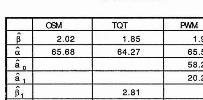
Estimated values of parameters for sample number 1 using

various methods.

06M TOT PWM

p 2.02 1.85 1.90

a 65.68 64.27 65.59

^0 58.20

a i 20.20

Pi 2.81

kn 1.40

s 12.

Table 2.1b

Estimated values of parameters for sample number 2 using

various methods.

06M TOT PWM

P 10.27 9.74 11.24

a 730.43 723.41 727.77

ap 695.67

327.03

Pi 10.61

kn 1.40

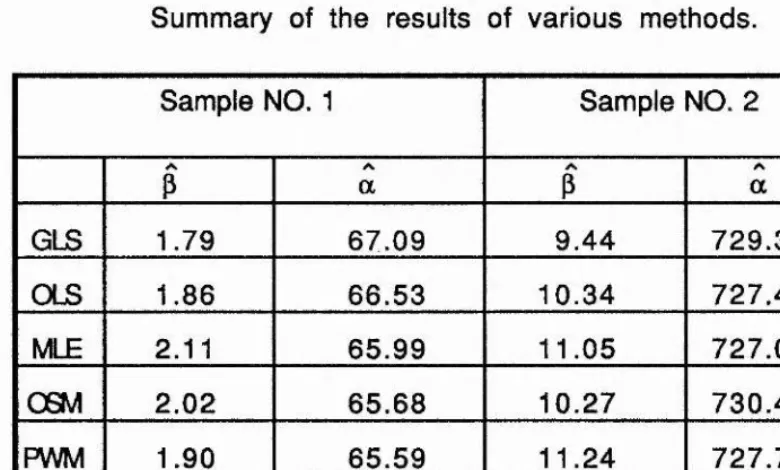
The results of all seven methods are summarized in table 2.2

Table 2.2

Summary of the results of various methods.

Sample NO. 1 Sample NO. 2

P a P a

GLS 1.79 67.09 9.44 729.36

OLS 1.86 66.53 10.34 727.40

MLE 2.11 65.99 11.05 727.07

OSM 2.02 65.68 10.27 730.43

PWM 1.90 65.59 11.24 727.77

TOT 1.85 64.27 9.74 723.41

!

2.3 .2

Several ceramic data sets are used to illustrate the range of

the shape parameter p which is considered in this chapter, and

to fit the data. Tables 2.3a and 2.3b show the estimated values I

of the two parameters of the Weibull distribution, along with

the Anderson Darling (A^) goodness of fit statistic, as obtained

by (a) GLS and (b) MLE. Figures 2.1-2.2 illustrate goodness of fit

for two data sets with large shape parameter values.

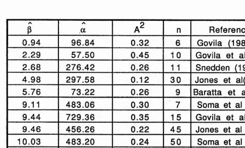
The Anderson Darling test statistic for the two-parameter

Weibull distribution takes values between 0.08 and 0.58 for all

data sets which are used. Use of critical values for case 3 will

lead to acceptance of this distribution at the 5% level, from

Table 4.17 of D'Agostino and Stephens (1986), for which values

are estimated by MLE. For sample size n=10 the critical value

for a test of goodness of fit at 0.05 significance level is 0.712.

Therefore, the two-parameter Weibull distribution is accepted

as a model for the three data sets with n=10. Similarly,

assuming that the same tables are applicable when estimation

is by GLS, it is an acceptable fit for the other data sets in Table

Table 2.3a

GLS for the two-parameter Weibull distribution, and

Anderson-Darling statistic values.

p a a2 n Reference

0.94 96.84 0.32 6 Govila (1982)

2.29 57.50 0.45 10 Govila et al(1985)

2.68 276.42 0.26 11 Snedden (1989)

4,98 297.58 0.12 30 Jones et al(1979)

5.76 73.22 0.26 9 Baratta et al(1974)

9.11 483.06 0.30 7 Sema et al (1986)

9.44 729.36 0.35 15 Govila et al(1985)

9.46 456.26 0.22 45 Jones et ai (1979)

10.03 483,20 0.24 50 Soma et al (1986)

10.64 418.92 0.53 45 Jones et al (1979)

12.98 414.49 0.48 10 Soma et al (1986)

13.70 541.66 0.44 10 Soma et al (1986)

Table 2.3b

MLE for the two-parameter Weibull distribution, and

Anderson-Darling test statistic values.

p a A= n Reference

1.31 91.63 0.34 6 Govila (1982)

2.82 56.60 0.38 10 Govila et al(1985)

3.25 272.16 0.23 11 Snedden (1989)

5.56 296.59 0.08 30 Jones et al (1979)

7.31 72.64 0.26 9 Baratta et al (1974)

11.85 481.50 0.40 7 Soma et al (1986)

11.05 727.07 0.32 15 Govila et al(1985)

10.19 455.92 0.20 45 Jones et al (1979)

10.73 482.58 0.21 50 Soma et al (1986)

11.44 418.69 0.58 45 Jones et al (1979)

15.638 413.09 0.48 10 Soma et al (1986)

14-1 2

-1 0

-] - — J 1—: , r-»-| pi—,—

250 300 350 400 450 500 550 600

Figure 2.1a Histogram of the ceramic data of size 50 and pdf

0.8“

0.6“

0.2

-0.0

250 300 350 400 450 500 550 600

CDF EOF

Data

Figure 2.1b Gdf and Edf of the ceramic data of size 50

14-1 2

-1 0

-250 300 350 400 450 500 550 600

Figure 2.1c Histogram of the ceramic data of size 50 and pdf

1.0

0.8

-0.6

-

0.4-0.2

-0.0

250 300 350 400 450 500 550 600

CDF

E O F

Data

Figure 2.Id Gdf and Edf of the ceramic data of size 50

of the two-parameter Weibull distribution fitted by MLE.

18-

16-

14-1 2

-10

-220 260 300 340 380 420 460 500 540 580

-ï

Figure 2.2a Histogram of the ceramic data of size 45 and pdf

1.0

0.8

-0.6

-

0.4-0.2

-0.0

2 2 0 2 6 0 300 340 380 420 460 500 5 4 05 80

CDF EDF

Data

Figure 2.2b Cdf and Edf of the ceramic data of size 45

of the two-parameter Weibull distribution fitted by GLS.

18-

1614

-1 2

-1 0

4

-220 260 300 340 380 420 460 500 540 580

Figure 2.2c Histogram of the ceramic data of size 45 and pdf

of the two-parameter Weibull distribution fitted by MLE.

0.8

-0.6

-0.4“

0.2

-0.0

220 260 300 340 380 420 460 500 540 580

CDF H F

Data

Figure 2.2d Cdf and Edf of the ceramic data of size 45

2.4 SIMULATION

2.4.1 Shape Parameter 0.5 < p < 4

One thousand (N) simulations were done for samples of sizes

10 and 25 with p= 0.5, 1, 2 and 4; and a = 0.1, 1, 10 and 100. The

random samples of Weibull data were generated using the

GENSTAT (Alvey et al 1980) random number generator. Goodness

of fit tests were applied to verify that the generated data

followed the parent distribution.

The choice of values of a, p, and sample size was made to

allow comparison with the results of other authors e.g. Engeman

and Keefe (1982), Gibbons and Vance (1981) and Gross and Lurie

(1977).

The methods are compared through properties of, (a) the

parameter estim ates, and (b), predicted quantités. The

parameter estim ates are assessed through their relative

efficiency (RE) and their mean squared error (MSE). The 95% and

99% quantité estimates are assessed through their relative bias

(RB) and mean squared relative error (MSRE).

M S E o f p = Ji S ( P i- p ) 2 (2.4.1)

1 = 1

- 1 ^ ^

MSE of a =1 1 (a j - a )2 (2.4.2)

i = 1

RE of p = [0.608 (p2)/n]/MSE (g) (2.4.3)

RE of a = [1.109 (a/p)2/n]/MSE (a) (2.4.4) !

1 N t p.

R B = ;i 2 (“ T—^ -1) , where p= 0.95 or 0.99 (2.4.5)

1 = 1 P

Leone et al. (1960) conjectured that the percent bias in p

was independent of the values of a and p. This was confirmed

for OLS and HAZ by Bain and Antle (1967). They defined p^^ and

as estimators for p and a obtained by OLS or HAZ when

sampling from a Weibull distribution with a = 1 and p = 1, and

proved the following theorem

" Let t.|, ... , t^ denote a random sample from a Weibull

distribution, w(t; a, P), and let a and p given by OLS or HAZ, then:

(1) p /p has the same distribution as p ^ ^ and is therefore

independent of a and p.

1 N t n i 2 -I

MSRE=7j £ ( - ^ - 1 ) (2.4.6)

1=1 P '

Table 2.4 shows the RE of the estimates of the parameters by

each of methods 1-4, for 16 pairs of parameter values. It is

noted that the RE for a particular method is almost independent

of the scale parameter a whether a or p is being estimated, and

I

that the RE of the estimate of p is independent of the value of p. f

Thus table 2.4 can be summarized in Table 2.5.

(2) a /a has the same distribution as and thus depends only on p

(3) p ln(a/a) has the same distribution as In or (a/a)^

has the same distribution as .

Similarly for MLE, Thoman, Bain and Antle (1969) showed in

their Theorem A, that ^ /p was distributed independently of a and p.

Therefore, for these three methods, the RE of p is

independent of both a and p, and the RE of a is independent of a.

For GLS, the location and scale parameters may be estimated

by solving n linear equations of the form given at the begining of

section 2.2.1.

These n equations may be written in matrix format as :

= (H' »' V ^Y

where K is an n x 2 matrix (1, E(kI));

V is the variance-covariance matrix (n x n);

and Y is a vector of ordered observations (n x 1).

Using general linear model theory (Graybill 1976) the variance

matrix of the estimators of Ç and 0 can be approximated by

D

where

as in Engeman and Keefe (1982).

Hence

v a r ( 0 ) = - ; ^

as derived by Lloyd (1952) for estimation of location and scale

parameters.

Similarly, for Ç

var(Ç) =

Now p = 1/0, hence

A -6^

ÔP — ^ 2

0^ Therefore

var(0)

var(P) = ^4

i.e. var(p) = p var(0) = — ^ - „+2

var(p/p)= ^

Now 0 = E(0) + 60

where 60 is the deviation of 0 from E(0).

Then

1 1

0 E(0) + 60

1 = { E ( ê ) [i

8 E{8)

i _{/ s [ 1 “ /\ + ( /\ ) - . . . ]}r . ; 58 2 ,

0 E(0) E(0) E(0)

E(p) = p [ 1

0

>22

E(P/P) - 1 +

Therefore the variance of p /p and the bias of p/ p, are

independent of p and a; also the RE of p/p is independent of p

and a.

Since a = exp (Q

6& = [ E x p ( g ) ] 6C

var(a ) « var(Ç)

var{a/a) =

Now a = exp [ (E(Ç)) + 5^ ]

{ S t y

a ~ exp(E(Ç)) [ 1 + + gi + ••• ]

|1 1

Therefore the variance of a /a and the bias of a / a are

independent of a; also RE of a / a is independent of a .

Table 2.4

Observed relative efficiencies for estimators of Weibull

parameters p and a (n=25).

Es imators of p Estimators of a

P a 0.1 1 10 100 0.1 1 10 100

GLS 0.898 0.898 0.898 0.898 0.777 0.778 0.778 0.778

0.5 OLS 0.865 0.665 0.665 0.665 0.731 0.731 0.731 0.731

HAZ 0.682 0.682 0.682 0.682 0.921 0.921 0.921 0.921

MJE 0.740 0.740 0.740 0.740 0.827 0.828 0.828 0.828

GLS 0.898 0.898 0.898 0.898 0.945 0.945 0.946 0.946

1 OLS 0.665 0.665 0.665 0.665 0.908 0.909 0.909 0.909

HAZ 0.682 0.682 0.682 0.682 0.989 0.989 0.989 0.989

MLE 0.740 0.740 0.740 0.740 0.971 0.971 0.971 0.971

GLS 0.898 0.898 0.898 0.898 0.988 0.988 0.988 0.988

2 OLS 0.665 0.665 0.665 0.665 0.961 0.962 0.962 0.962

HAZ 0.682 0.682 0.682 0.682 0.968 0.968 0.968 0.968

MΠ0.741 0.740 0.740 0.740 0.996 0.996 0.996 0.996

GLS 0.898 0.898 0.898 0.898 0.996 0.996 0.996 0.996

4 OLS 0.665 0.665 0.665 0.665 0.976 0.977 0.976 0.976

HAZ 0.682 0.682 0.682 0.682 0.945 0.946 0.945 0.945

Table 2.5

Average relative efficiency of each estimator across

param etrizations

Estimator Estim ator

Method of p of a when

P = 0.5 P = 1 p = 2 p=4

GLS 0.898 0.778 0.945 0.988 0.996

OLS 0.665 0.731 0.909 0.962 0.976

HAZ 0.682 0.921 0.989 0.968 0.945

i

achieved by the GLS estimator, while the OLS estimator has the |

lowest average RE. The results for estimating a are less clear

cut. For p less than or equal to 1 the HAZ method is clearly most -|

efficient. For p = 2 the MLE method is better than GLS but all

four methods are very efficient. For p = 4 GLS is slightly better

than MLE, and again, all four methods are very efficient.

Our results shown in Table 2.6 are in broad agreement with I

those in Table I of Gross and Lurie (1977) so far as bias and 4

standard deviation of p are concerned. But we disagree with

their bias and standard deviation for a. We do agree with

corresponding results shown in Table I of Gibbons and Vance

(1981) for the variance of a estimates by MLE. (Table 2.7).

The RMSE of parameter estimates can be seen in Table 2.6. It

is clear that the GLS method produces smaller RMSE for p,for

both sample sizes 10 and 25, than any other method.

For GLS method, the difference between the theoretical

relative bias and the simulation result in Table 2.6 is due to the

choice of plotting position i/(n+1). This plotting position was

used in the simulation to enable comparison between its result

and those of Engeman and Keefe (1982). Other plotting positions

(e.g. (i-0.01)/n) may give different relative bias.

For example, using simulation with P;=(i-0.01)/n, p = 1, a = 1

and n = 25, the relative bias in p is 0.028, and the variance of

Theoretically, with this plotting position, = 0.6794 and hence

E[ ( p / P ) - 1 ] « “ » v a r ( “ ) « 0.025

Thus, it can be seen that, under these conditions, the plotting

position Pj=(i-0.01)/n gives results that are in good agreement

Monte Carlo simulation of the Weibull parameters based on

1000 random samples, with sample size n, shape parameter p,

scale parameter a, standard deviation (SD), bias, and root mean

square error (RMSE) for both parameters

n 10 10 10 25 25 25

P 0.5 1 5 0.5 1 5

a 1 1 1 1 1 1

Bias in p MLE 0.076 0.152 0.761 0.027 0.054 0.273

HAZ -0.020 -0.040 -0.201 -0.021 -0.043 -0.213 OLS -0.037 -0.075 -0.373 -0.030 -0.060 -0.301 GLS -0.037 -0.074 -0.371 -0.027 -0.055 -0.271

Bias in a MLE 0.105 -0.003 -0.009 0.049 0.002 -0.003

HAZ -0.039 -0.072 -0.024 -0.011 -0.028 -0.009

OLS 0.206 0.042 -0.001 0.098 0.025 0.001

GLS 0.173 0.029 -0.003 0.076 0.015 -0.001

SD of p MLE 0.167 0.334 1.670 0.087 0.173 0.865

HAZ 0.158 0.315 1.577 0.092 0.184 0.921

OLS 0.153 0.308 1.532 0.091 0.182 0.908

GLS 0.135 0.271 1.354 0.078 0.155 0.777

SD of a MUE 0.761 0.332 0.066 0,461 0.214 0.042

HAZ 0.679 0.315 0.067 0.349 0.210 0.042

OLS 0.826 0.346 0.067 0.483 0.219 0.043

GLS 0.798 0.339 0.066 0.472 0.216 0.042

RMSEofp MLE 0.183 0.367 1.833 0.091 0.181 0.907

HAZ 0.159 0.318 1.589 0.094 0.189 0.944

OLS 0.158 0.315 1.576 0.096 0.191 0.956

GLS 0.140 0.281 1.403 0.082 0.165 0.823

RMSEofa MLE 0.768 0.332 0.067 0.463 0.214 0.042

HAZ 0.679 0.323 0.071 0.439 0.212 0.043

OLS 0.850 0.349 0.067 0.493 0.221 0.043

GLS 0.817 0.341 0.066 0.478 0.217 0.042

1

»

I

Table 2.7

Estimated variance of a when a =1

sample

size P

M_E HAZ OLS GLS

10 0.5 0.579 0.461 0.682 0.637

10 1.0 0.110 0.099 0.119 0.115

10 5.0 0.004 0.004 0.004 0.004

25 0.5 0.213 0.193 0.233 0.222

25 1.0 0.046 0.044 0.048 0.047

25 5.0 0.002 0.002 0.002 0.002

Estimated variance of p

sample

size P

MLE HAZ OLS GLS

10 0.5 0.028 0.025 0.023 0.018

10 1.0 0.112 0.099 0.094 0.073

10 5.0 2.786 2.487 2.347 1.833

25 0.5 0.008 0.008 0.008 0.006

25 1.0 0.030 0.034 0.033 0.024

"fi

Table 2.4 refers to the same situations as found in Table I of

Engeman and Keefe (1982). There is little agreement between i

our results and theirs. Given that it has been shown that the RE

of ^ is independent of a, their table lacks coherence when p is

considered across a, and the RE of a is generally greater than 1.

They suggested that mixed methods might be able to improve on

a single method. From our results combinations of GLS for p

with either HAZ or MLE for a, depending on the value of p, are

possibilities. Thus we propose MM1, i.e. GLS for p then HAZ for

a if p < 1, and MM2, i.e GLS for p then MLE for a, if p > 1. The 1

results of using these methods is shown in Table 2.8 for 1000 |

simulated samples of size 25 and p = 0.5, 1, 2, 4.

Table 2.8

Result of 1000 simulations to compare four methods of

estimation through the relative efficiency (RE) for estimators

of p and a, the relative bias (RB), and the mean square relative

error (MSRE) of the predicted 95% and 99% quantiles.

RE of

estimating

RB RB MSRE MSRE

p P a T95 T99 T95 T9 9

0.5 GLS 0.898 0.777 0.330 0.516 0.550 1.184

OLS 0.665 0.731 0.517 0.881 1.497 4.901

HAZ 0.682 0.921 0.281 0.616 0.873 2.644

MLE 0.740 0.827 0.004 0.021 0.223 0.338

MM1 0.898 0.899 0.224 0.382 0.412 0.868

1 GLS 0.898 0.945 0.121 0.179 0.088 0.156

OLS 0.665 0.909 0.174 0.264 0.169 0.353

HAZ 0.682 0.989 0.086 0.153 0.116 0.234

MUE 0.739 0.971 -0.023 -0.025 0.051 0.071

MM1 0.898 0.978 0.074 0.129 0.072 0.125

2 GLS 0.898 0.988 0.051 0.074 0.019 0.030

OLS 0.665 0.961 0.071 0.104 0.032 0.057

HAZ 0.682 0.968 0.031 0.068 0.023 0.041

MLE 0.741 0.996 -0.018 -0.021 0.013 0.018

MM2 0.898 0.966 0.023 0.045 0.015 0.025

4 GLS 0.898 0.996 0.023 0.034 0.004 0.007

OLS 0.665 0.976 0.032 0.046 0.007 0.012

HAZ 0.682 0.945 0.013 0.029 0.005 0.009

MLE 0.740 0.995 -0.011 -0.013 0.003 0.005

MM2 0.898 0.929 0.009 0.019 0.004 0.006

i

I

These results are somewhat disappointing because the RE of

the estimate of a is not as large as that for a estimated by

separate use of HAZ i.e. with its corresponding value of p, or of

MLE when p is larger. However if a method is sought that gives

good estimates of both p and a, the mixed method is better than

any single method of 1-4.

Turning to the predicted quantiles, the RB and MSRE for four

values of p and for sample size 25 are summarized in Table 2.8.

MLE is clearly the best method for all values of p. The second

best is MM 1/2, and the worst is OLS.

2.4.2 Shape Parameter p < 30

A simulation study was conducted in order to compare the six

methods (GLS, OLS, MLE, OSM, TQT and PWM ). For each of the

shape parameter values p= 0.5, 1, 2, 5, 10, 20 and 30, one

thousand random samples of size 10 and 25 were generated from

a Weibull distribution with a = 1. The random number generator

used was that in the GENSTAT package (Alvey et al 1980). The

methods are compared as in the previous section through the

parameter estimates and 95% and 99% quantiles as found in

equations 2.4.1,..., 2.4.6. To facilitate comparisons, the results

of the simulation are presented graphically. Figures 2.3, 2.4, 2.5

and 2.6 show RE of the estimates of parameters by each of

methods 1, 2, 4, 5, 6 and 7 for different values of the shape

parameter. As expected, the efficiency of each method of

a few cases it can be seen that the RE is greater than 1.

However these discrepancies are very small and can be If

attributed to sampling fluctuations in the relatively small

variance of the scale parameter a. The graphs of the product of

the RMSRE and p, against p, is shown in Figures 2.7, 2.8, 2.9 and

2.10. This product is used because it varies over a smaller range

than do the RMSRE.

For estimating the shape parameter, it is evident from

Figures 2.3 and 2.4 that the GLS estimator is considerably more

efficient than the other methods for both sample sizes, and that

efficiency increases with sample size. For most methods the i

,‘v

efficiency is independent of the shape parameter, the exception

being PWM. It is noteworthy that in both Figures the PWM l|

estimator had low RE at p =0.5, but high RE at p =1 and at p =2.

Generally speaking, the second best method for estimating p is

CJ z LU H—( LJ H -H Li_ li_ LU n=1 0

SHAPE

1 .0 0

0.95 0. 90 0. 85 0.80 □B-0-0.75 0.70 0.65 0.60 0.S5 0.50 0.45 0.40 30 25

0 5 10 15 20

a

i

Figure 2.3 Empirical efficiency of estimates of shape

parameter by various methods, from simulated sample of size

n=25 >-o z UJ »— I o_I—I ÜL. Li_ UJ 1.00 0.95 0.90 0.85 0.80 0. 75 0.70 0.65 0.60 0.55 0.50 0.45 0.40 30 15

GLS □

OSM *

MLE

GLS e

PWM •

TOT

20 25

SHAPE

30 ■QB-B

G B -e

Figure 2.4 Empirical efficiency of estimates of shape

parameter by various methods, from simulated sample of size

25.

The RE of a is less clear cut, as seen in Figures 2.5 and 2.6.

For 2 < p < 30 the GLS method is better than the other five

methods, and the TOT method is worse than the other methods.

For p < 2, and n=10, OSM and TOT are the most efficient

methods, but when p < 2 and n= 25, TOT is best, followed by MLE.

n ;

4

I

n= 1 0

LU

>—i L J 0.9S I—I u_ u_ U J

0.90

0.85

0.80

0.75

0.70

0.60

0 5 10 15 20 25 30

SHAPE

4

Figure 2.5 Empirical efficiency of estimates of scale

parameter by various methods, from simulated sample of size

L J Z UJ 1—4 LJ ►—4 u_ Lu LU n=25 1.00 0.95 0. 90 0.85

GLS

OSM

MLE

OLS

PWM

TOT

0 5 10 15

SHAPE

Figure 2.6 Empirical efficiency of estimates of scale

parameter by various methods, from simulated sample of size

For estimating the sample quantiles, the method is sought

that has smallest RMSRE. From Figures 2.7, 2.8, 2.9, and 2.10 it

is evident that unless p < 1, MLE is the best method, followed

closely by TQT. For p < 1 Figures 2.7 and 2.8 show that PWM is

the best method for the 95% quantile, with OSM as a close

competitor, while Figures 2.9 and 2.10 show that OSM is the

best method for the 99% quantile. In all of the Figures 2.7, 2.8,

n=10

0.9

0.7

0.6

0.5

0.4

0.3

0.2

0 5 10 _{IS 20 25 30}

SHAPE

Figure 2.7 The root mean square relative error of estimates

of the 95% percent quantile with parameters estimated by

various methods from simulated sample of size 10.

3

n=25

1.0

0.9

GLS □

OSM *

MLE A

OLS o

PWM •

TQT X

0.7

0.6

0.5

0.4

0.3

0.2

0.1

0 5 10 15 20 25 30

SHAPE

Figure 2.8 The root mean square relative error of estimates

of the 95% percent quantile with parameters estimated by

various methods from simulated sample of size 25.

I

n=1 0

SHAPE

Figure 2.9 The root mean square relative error of estimates

of the 99% percent quantile with parameters estimated by

various methods from simulated sample of size 10.

0.8

0.7

0.6

0.5

0.4

0.3

0.2

0.1

0 5 10 15 20 25 30

■I

n=25

SHAPE

Figure 2.10 The root mean square relative error of estimates

of the 99% percent quantile with parameters estimated by

various methods from simulated sample of size 25.

GLS

OSM

MLE

OLS

PWM

TQT

0.9

0.6

0.7

0.6

0.5

0.3

0.2

30

0 5 10 15 20 25

B variability in the RE of ]3

♦ variability in the RE of a

0,00 0.02 0.04 0.06 0.08 0.10 0.12

1/N

Figure 2.11 Variability of RE for shape and scale parameters

using GLS.

It can be seen from Figure 2,11 that the variance of RE is

inversely related to the number of simulations.

For GLS with sample size 25 and with 1000 simulations the

RE for p (and for a) has coefficient of variation less than 4%

(and 5%).

1