An Improved Algorithm for Finding the Anti-block Vital Edge of a Shortest Path

An Improved Algorithm for Finding the

Anti-block Vital Edge of a Shortest Path

Zhe Nie

Yueping Li, Member IAENG

Abstract—This paper presents an improved algo-rithm to find the anti-block vital edge of a shortest path. We release the constraint that there is only one shortest path between two nodes introduced by Su, Xu and Xiao. We use the technique developed by Nardelli, Proietti and Widmayer and give a im-provement in search strategy. Our algorithm runs in

O(m+nlogn) time which is superior to the previous one whose complexity is in O(mn), where n and m

denote the number of nodes and edges in the graph. In addition, our algorithm can be further improved to run in O(mα(m, n)) time, whereαis the functional inverse of the Ackermann function.

Keywords: graph algorithms, shortest path, detour, critical edge

1

Introduction and Preliminary

The survivability of communication network is a critical issue. It has been studied intensively. We focus on a par-ticular type of it: How is a network affected by an edge (link) failure? Our scenario assumes that we route along a shortest path in the network from the source to the des-tination. When an edge fails, we need to choose another path, which probably is a shortest path does not contain the failed edge. This problem is calledpath replacement

in literature [1]. From the management point of view, it is valuable to evaluate the effect by the failure of a link. The classical problem is to find amost vital edge(MVE): the edge whose removal results in the largest increase of the length with respect to a shortest path. Corley and Sha [3] proposed anO(mn+n2logn) time algorithm to solve this problem. And a more effective algorithm was developed by Malik, Mittal and Gupta [5] which runs in O(m+nlogn) time.

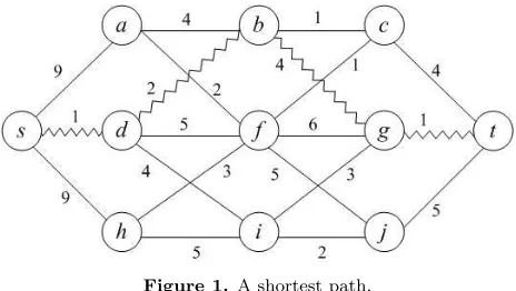
Most previous works paid attention to the length of the replacement path minus the length of the shortest path. For example, the shortest path from sto t isPG(s, t) =

s, d, b, g, twhich is illustrated with wavy lines. We denote the length of pathP by|P|. So we have|PG(s, t)|= 8. It

is easy to verify that the edge (s, d) is the most vital edge. We havePG−(s,d)(s, t) whose length is 16. Thus, the edge

∗_{Zhe Nie: Shenzhen Polytechnic, Xili, Shenzhen P.R. China} 518055 Email:niezhe@oa.szpt.net; Yueping Li: Sun Yat-sen Uni-versity, Department of Computer Science, Guangzhou P.R. China 510275, Email: leeyueping@gmail.com

(s, d) is critical. However, Su, Xu and Xiao [8] proposed a different parameter for measuring the vitality of an edge of a shortest path. They focused on an edgee= (u, v) in PG(s, t) whose removal produces a replacement path at

vertex u such that |PG−e(u, t)|/|PG(u, t)| is maximum.

They defined such an edge as the anti-block vital edge (AVE for abbreviation).

Figure 1.A shortest path.

Our scenario is that a traveller may reach a vertex u but the edge (u, v) which is intended to pass fails sud-denly. The traveller will route from u to t through a shortest path PG−(u,v)(u, t). It is natural that the

max-imum ratio is one of the key parameters for measur-ing a route strategy. For instance, if the edge (s, d) is failure, |PG−(s,d)(s, t)|/|PG(s, t)| = 2. However, if the

edge (g, t) is not available,|PG−(g,t)(g, t)|/|PG(g, t)|= 9.

It implies that the edge (g, t) is more important than the edge (s, d) from this measure of view. Note that the increase length of |PG−(s,d)(s, t)| − |PG(s, t)| equals

|PG−(g,t)(g, t)| − |PG(g, t)| whose value is 8. Hence, the

edges (s, d) and (g, t) have no difference with respect to the increase of the length of a shortest path.

This paper is organized as follows: In Section 2, we de-fine the problem formally. In Section 3, our algorithm is presented. In Section 4, an improvement is given. Ex-perimental results and analysis are proposed in Section 5 and 6, respectively. Finally, the conclusions and future works are given in Section 7.

2

Definition and Terminology

Letw(e) be a positive real length for each edgee∈E(G). A graphH = (V(H), E(H)) is called a subgraph ofGif V(H)⊆V(G) andE(H)⊆E(G). And ifV(H) =V(G), H is said to be a spanning subgraph ofG.

A connected acyclic spanning subgraph of Gis called a spanning tree of G. A single-source shortest paths tree (SPT)SG(r) is a spanning tree ofGrooted atrand

con-sisting of the union of the shortest paths. It is straight-forward that there is exactly one shortest path fromrto v for eachv∈V(G\r).

A graph Gis connected if there exists a path from uto v for any two vertices u, v ∈ V(G). We call a graphG 2-edge-connected if G−eis connected for any edge e∈

E(G). We consider undirected 2-edge-connected graphs in this paper.

Let PG−e(s, t) be a shortest path between s and t. As

mentioned above, we callPG−e(s, t) a replacement

short-est path forv. Denote its length bydG−e(s, t).

The anti-block coefficient of an edgee= (u, v)∈PG(s, t)

is the ratio cu,t ofdG−e(u, t) todG(u, t).

The anti-block vital edge (AVE) with respect toPG(s, t)

is the edge e0 _{= (u}0_{, v}0_)∈P

G(s, t) whose removal results

in cu0,t0 ≥cu,t for any edgee= (u, v) ofPG(s, t).

3

Description of the Algorithm

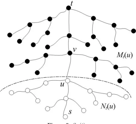
Su, Xu and Xiao [8] proposed anO(mn) time to find the anti-block edge with respect to a shortest path. But they assumed that there is only one shortest path between the source sand the destination t, which has limited appli-cation. We eliminate this constraint and develop a more effective algorithm.

Figure 2.SG(t).

At first, we compute the shortest path treeSG(t) rooted

at t. It is natural to develop an algorithm by building SG−e(t) for eache∈PG(s, t) which runs inO(mn) time.

The reader can refer to Su, Xu and Xiao [8]. However, it is too expensive. In the light of [7], we adopt the Fibonacci heaps [4] in order to improve the algorithm to run in O(m+nlogn) time.

Lete= (u, v) be an edge ofPG(s, t) where the vertexu

is closer tosthanv. LetMt(u) denote the set of vertices

reachable inSG(t) fromtavoiding passing the edge (u, v).

Let Nt(u) = V(G)−Mt(u). An example of Mt(u) and

Nt(u) is illustrated in Fig. 2. It is straightforward that

for any vertexxinMt(u), we havedG−e(x, t) =dG(x, t).

We define the edges between the partition Nt(u) and

Mt(u) as follows:

Et(u) ={(x, y)∈E(G)−(u, v)|x∈Nt(u) and

y∈Mt(u)}.

Suppose the traveller has arrived at the vertex u, but the edgee= (u, v) fails at that time. Then the traveller has to route avoiding the edge e. That is, the detour PG−e(u, t) must contain an edge in Et(u) of which an

example is shown in Fig. 3. It implies that the length of detour satisfies the following formula:

dG−e(u, t) = min (x,y)∈Et(u)

{dG−e(u, y)+w(x, y)+dG−e(x, t)}

(1) .

Figure 3. A detourPG−(u,v)(u, t).

From the structure ofSG(t), it implies thatdG−e(u, y) =

dG(y, t)−dG(u, t). Note thatdG−e(x, t) =dG(x, t). Thus,

Formula (1) can be computed inO(1) time. Since we can check each edge in Et(u) in O(m) time, it is

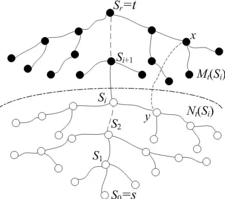
and Widmayer [7]. Suppose the pathPG(s, t) iss0(=s),

s1,. . ., sr−1,sr(=t) andei= (si, si+1).

For each ei, we adopt a Fibonacci heap to build a

priority queue whose element stores the shortest path PG−ei(si, t). In the light of Formula (1), we use Qi(y)

to record the shortest path passing through the vertexy and avoiding the edgeei. We define

Qi(y) = min (x,y)∈Et(si)

{dG(t, x) +w(x, y) +dG(y, si)} (2)

It is clear that we need to maintain the queue Qi for

the vertices ofNt(si) only. Note thatNt(si)⊂Nt(si+1).

Hence, we seti=rand calculateQr(y) at the first step.

Sincei=r, the edgeeiis empty. Thus,Qr(y) just records

the value ofdG(y, t). Once the queueQi(y) is calculated

out, we continue to computeQi−1(y) wherei >0.

Figure 4. SiandSi+1.

Nardelli et al. [7] pointed out if we use Formula (2) as a key of the priority queue, the cost will be expensive, since when the next edge ei−1 is considered, we have to

decrease the value by w(ei−1) for all the elements in the

queue. Thus, they gave the appropriate key as follows:

Ki(y) = min (x,y)∈Et(si)

{dG(t, x) +w(x, y) +dG(y, s)} (3)

It is clear that if the vertex y remains in Nt(si−1), the

valueKi(y)−dG(t, si−1) still records the length of a

can-didate path. We now give the procedure of the algorithm introduced by Nardelli et al. [7].

Nardelli’s Algorithm

Input: A graph Gwith a shortest pathPG(s, t)

Output: dG−efor anye∈E(PG(s, t))

(1) Build a shortest path tree rooted at t, denoted bySG(t)

(2) LetK(y) =dG(s, t) for ally∈V(G)

and build a Fibonacci heap usingK(y) as key (3) SupposePG(s, t) =s0(=s),s1,. . .,sr−1,sr(=t)

(4) Leti=randei= (si, si+1)

(5) whilei >0 do (6) Begin

(7) LetS be the set ofNt(si)−Nt(si−1)

(8) Remove the keyK(x) from the heap ifx∈S (9) For each x∈S, search its neighbors:

If there is an edge (x, y) wherex∈Nt(si−1),

we computedG(t, y) +w(y, x) +dG(x, t);

If the value is less thanK(y), we assign it toK(y) (10) Letc be the minimum key of the heap (11) LetdG(si−1, t) =c−dG(t, si−1)

(12) Decreaseiby 1 (13) End(while)

Since the values of dG−e for any e ∈ E(PG(s, t)) have

been obtained, it is easy to calculate the maximum anti-block coefficient along the edges ofPG(s, t). That is, we

can determine the anti-block edge in this way.

4

Improvement

In this section, we propose an improvement of the search strategy and discuss the time-space trade-off. The fastest algorithm to perform Step (1) introduced by Fredman and Tarjan [4] adopts the adjacent list to store the graph. It runs inO(m+nlogn) time.

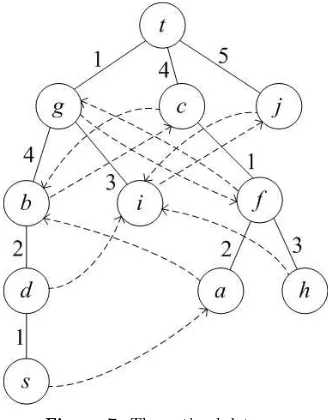
It is well known that the adjacent list can be implemented by means of link list. Furthermore, we add two links between the two instances which stand for the same edge in graph which is shown in Fig. 5. Furthermore, we maintain the array which stores the tails of the link list of certain vertices.

Figure 5.The structure of adjacent list.

We change Step (9) as follows:

(9.1) Let ebe the first edge in the list. (9.2) whilee <> N ulldo

(9.3) Begin if eis marked, then break; (9.4) Supposee= (x, y);

(9.5) If x ∈ Nt(si−1), we compute dG(t, y) +w(y, x) +

dG(x, t);

(9.6) If the value is less thanK(y), we assign it to K(y); (9.7) Mark the edgee;

(9.8) Move eto the tail of the link list of the vertexy;

We use morenunits of space to store the tail of the link list of each vertex. But we avoid to search one edge twice. Thus, the improved algorithm diminishes the complexity by m units of time. Since m is in O(n2_{) usually, our}

improvement makes sense.

Our improvement above focuses on the time-space trade-off. We now propose a method to perform Step (8) effec-tively and then present an alternative method which uses less space but takes more time. As known, it is expensive to locate the node which is associated with the vertex y in Fibonacci heap since the key isK(y) noty. Hence, we also use an array to record the node in the heap for each vertex in the graph. But if we prefer space to time, we does not record the position of the corresponding node for each vertex. We eliminate Step (8) and change Step (10) as follows:

(10.1) Letcbe the minimum key of the heap;

(10.2) Ifcis the value ofK(y) and the vertex yis not in Nt(si−1), then delete the keyc and Goto Step (10.1);

It implies the alternative algorithm sparesnunits of space but takes more time for the operations of the Fibonacci heap. However, the time complexity remains in O(m+ nlogn).

5

Experimental Results

Figure 6.The shortest path tree.

The shortest path tree of the graph in Fig. 1 is shown in Fig. 6. The optimal detours are shown in Fig. 7 for each vertex when the edge from the vertex to its parent fails. The first edges of the detours are marked with dotted lines.

Figure 7. The optimal detours.

And the following table presents the lengths of the opti-mal detours.

Table 1: PG(x, t),dG−(x,y)(x, t) andcx,t

Edge(x, y) PG(x, t) dG−(x,y)(x, t) cx,t

(s, d) 8 16 2

(d, b) 7 8 8/7

(b, g) 5 5 1

(g, t) 1 9 9

(i, g) 4 7 7/4

(a, f) 7 9 9/7

(h, f) 8 9 9/8

(f, c) 5 7 7/5

(c, t) 4 6 3/2

(j, t) 5 6 6/5

(b, c) 5 5 1

(c, t) 4 6 3/2

As mentioned in Section 1, though dG−(g,t) =dG−(s,d),

the anti-block coefficient of the edge (g, t) is much larger than the one of (s, d). So the edge (g, t) is critical in the path. From this point of view, we had better choose the shortest path to beP =s, d, b, c, t. The maximum anti-block coefficient ofPis 2 since thecb,t = 1 andcc,t= 3/2

with respect to the edges (b, c) and (c, t), respectively. Thus, the route of P is better than the route s, d, b, g, t which is shown in Fig. 1.

6

Analysis of the Algorithm

According to Nardelli’s algorithm, it can be concluded that it has no limitation on the number of the short-est path from the source to the dshort-estination. Thus, so does our algorithm. It is clear that our algorithm runs in O(m+nlogn) time andO(m) space.

The two alternative improved algorithms make exchange between time and space. And they both do not change the time and space complexity of the original algorithm.

7

Conclusions and Future Works

We propose an improved algorithm to find the anti-block vital edge of a shortest path. And the constraint in the previous algorithm [8] is eliminated. Our algorithm runs inO(m+nlogn) time which is faster than the one in [8] whose complexity isO(mn).

In addition, Nardelli, Proietti and Widmayer [6] im-proved their algorithm using a linear time algorithm for the shortest path tree by means of atransmuter[9]. They gave an O(mα(m, n)) time algorithm. Thus, Our algo-rithm can also be implemented in this way.

Bhosle and Gonzalez [2] found the replacement paths for all tree edges of a shortest path tree in O(m+nlogn) time. Thus, our algorithm can be extended based on their technique.

References

[1] Bhosle, A.M., “Improved algorithms for replacement paths,”Operatjions Research Letters, V33, pp. 459-466, 2005

[2] Bhosle, A.M., Gonzalez, T.F., “Algorithms for sim-ple link failure recovery and related problems,” Jour-nal of Graph Algorithms and Applications, V8, N3, pp. 275-294, 2004

[3] Corley, H.W., Sha, D.Y., “Most vital links and nodes in weighted networks,”Operation Research Letters, V1, pp. 157-161, 1982

[4] Fredman, M.L., Tarjan, R.E., “Fibonacci heaps and their uses in improved network optimization

algo-rithms,”Journal of the ACM, V34, N3, pp. 596-615, 1987

[5] Malik, K., Mittal, A.K., Gupta, S.K., “Thek most vital arcs in the shortest path problem,” Operation Research LettersV8, pp. 223-227, 1989

[6] Nardelli, E., Proietti, G., Widmayer, P., “A faster computation of the most vital edge of a shortest path between two nodes,”Information Processing Letters, V79, N2, pp. 81-85, 2001

[7] Nardelli, E., Proietti, G., Widmayer, P., “Finding the detour critical edge of a shortest path between two nodes,” Information Processing Letters, V67, N1, pp. 51-54, 1998

[8] Su, B., Xu, Q., Xiao, P., “Finding the anti-block vi-tal edge of a shortest path between two nodes,” In

Proceeding of COCOA 2007,Lecture Notes in Com-puter Science, V4616, pp. 11-19, 2007