An Inexact Implementation of Smoothing Homotopy Method for Semi Supervised Support Vector Machines

An Inexact Implementation of Smoothing Homotopy

Method for

Semi-Supervised Support Vector Machines

Huijuan Xiong, Feng Shi

College of Science, Huazhong Agricultural University, Wuhan, China Email: [email protected]

Received January 12, 2013; revised February 16, 2013; accepted February 25, 2013

ABSTRACT

Semi-supervised Support Vector Machines is an appealing method for using unlabeled data in classification. Smoothing homotopy method is one of feasible method for solving semi-supervised support vector machines. In this paper, an in- exact implementation of the smoothing homotopy method is considered. The numerical implementation is based on a truncated smoothing technique. By the new technique, many “non-active” data can be filtered during the computation of every iteration so that the computation cost is reduced greatly. Besides this, the global convergence can make better local minima and then result in lower test errors. Final numerical results verify the efficiency of the method.

Keywords: Semi-Supervised Classification; Support Vector Machines; Truncated Smoothing Technique; Global Convergence

1. Introduction

In the field of machine learning, it’s essential to collect a large amounts of labeled data for the purpose of train- ing learning algorithms. However, for many applica- tions, huge number of data can be cheaply collected, but manual labeling of them is often a slow, expensive and error-prone process. It’s desirable to utilize the unlabe- led data points for the implementation of the learning task. The goal of semi-supervised classification is to employ the large collection of unlabeled data jointly with a few labeled data to finish the task of classification and prediction [11,18].

Semi-supervised support vector machines (S3_{VMs) is} an appealing method for the semi-supervised classifi- cation. In [7], K.P. Bennett et al. first formulated it as a

mixed integer programming such that some state-of- the-art softwares can handle the formulation. Since that, a large number of methods have been applied to solve the non-convex optimization problem associated with S3_VMs, such as convex-concave procedures [5], non-differntiable methods [1], gradient descent method [13], continuation technique [12], branch-and-bound algorithms [7,14], and semi-definite programming [17] etc. A survey of these methods can be seen from [11,18].

As pointed out in [12], one reason for the large number of proposed algorithms for S3_{VMs is that the resulting} optimization problem is non-convex that generates local minima. Hence, it’s necessary to find better local minima because better local minima tend to lead to higher pre-

diction accuracy. In [12], a global continuation tech- nique is presented. In [21], a similar global smoothing homotopy method is given. However, both the method is experiential and the calculations are lengthy.

The focus of this paper is giving a new efficient im- plementation of the smoothing homotopy method for the S3_{VMs. In Section 2, we first introduce the new S}3_VMs model used in [21] and list two smoothing functions called aggregate function and twice aggregate function respectively. The two smoothing functions are given to approximate the nonsmooth objective function (the de- tailed discussion of these two smoothing functions can be seen from [4]). And then the smoothing homtopy method solving S3_{VMs is recalled. In Section 3, the new trun-} cated smoothing technique is established to give a more efficient pathfollowing implementation of the smoothing homotopy method. The new technique is based on a fact that, some “non-active” data do little effect on the value of the smooth approximation functions with their gra- dients and Hessian during the computation, as a result, these “non-active” data can be filtered by the new trun- cated technique to save the computation cost. With the inexact computation technique, only a part of original data is necessary during the computation of every itera- tion. In the last section, Two artificial data sets with six standard test data from [10] are given to show the effi- ciency of our method.

two vectors x and y in the n-dimensional real space

will be denoted by

n

R T

x y. For a matrix _A_Rm n _,

i

A

will denote the th row of i A. For a real number , a

a denotes its absolute value. For a vector xRn, 1

x denotes its 1-norm, i.e., ₁

1

n i i

x x







, x_

denotes its infty-norm, i.e.,

1

max i

i n

x_ x

 

 . For an index set I , I denotes the element number of it. For a

given function _{f R}: n 



R , if is smooth, its

gradient is denoted by

f



f x

 , if is nondifferential, denote its subdifferential as

f

 

f x

 .

2. Semi-Supervised Support Vector

Machines

There lies several formulations for S3_{VMs such as the} mixed integer programming model by K.P. Bennett et al.

[7], the nonsmooth constrained optimization model by O.L. Mangasarian [5], and the smooth nonconvex pro- gramming formulation by O. Chapelle [13] and etc. Here we mention the contributions by O. Chapelle et al. in

[11-14]).

Given a dataset consisting of m labeled points and p

unlabeled points all in , where the labeled points are represented by the matrix

n

R m

m n

A R 

 

B R

, p unlabeled

points are represented by the matrix and the labels for

p n

A are given by diagonal matrix

of _1. The linear S3_{VMs to find a hyperplane} mm T D

x b

 

far away from both the labelled and unlabeled points can be formulated as follows:



T 2











1 1 2 2

,

T

1 1

1

, ,

min 2

1 1

s.t.

b

p m

i ii

i i

b C f b C f b

B b D

p m

    



 

  

 

 

 









,

(1)

where













1 1

1

, m max 0, i ,

i

f  b f 







b













2 2

1

, p max 0, i ,

i

f  b f 







b





1 ,

i

f  b and _f2i



,_b



_{are loss functions corres-}

ponding to the labeled data and unlabeled data respec- tively and defined as follows,







T



1i , 1 ii i

f  b  D  A b





T

2i , 1 i

f  b   B b

where T

i

B b

  denotes the absolute value of . The constraint is called balanced constraint that is used to avoid unbalanced solutions which classify all the unlabeled points in the same class.

T

i B b  

For arbitrary vector , there lies an equivalent relation between its 1-norm and inf-norm in the sense

n

R



that 1 ₁

n       1, then the sum term of model (1)

can be substituted by the inf-norm form and model (1) can be reformulated as follows,



T 2











1 1 2 2

,

1 1

1

, ,

min ₂

1 1

s.t. b

p m

T

i ii

i i

b C f b C f b

B b D

p m

    



  

 

  

 

 

 









(2)

where











1 1

1

, max 0, i ,

i m



f  b f 

 

 b











2 2

1

, max 0, i ,

i p



f  b f 

 

 b .

We rewrite the constraint into the objective as a barrier term and reformulate ₂i



,



f  b into its equivalent for-

mulation







T T



2 , m ,1

i

i i

in 1

f  b   B b  B b , and

then obtain the following formulation that is our goal in the paper.



2















1 1 2 2 3

, 1

min , , ,

2

T

b b C f b C f b f b

        

where











1 , ₁max 0, 1 ,

i

i m



f  b f 

 

 b









1





2









2 , ₁max 0, min 2 , , ,

i i

i p 2

f  b f  b f

 

  b





1 T

2 , 1

i

i

f  b   B b





2 T

2 , 1

i

i

f  b   B b





T 2

3

1 1

1 1

,

p m

i i

i i

i

f b M B b D

p m

 

 

 

 _  _









M is a barrier parameter.

If the dataset is nonlinear separable, we need construct a surface separation based on some kernel trick (detailed discussion of it can be seen from [2] and etc.). Denote





T ;

A A B , assume that the surface we want to find is

 

,

K x A ub= 0, where is usually taken as

Gaussian kernel function with the form of

 

, K  

 



2



, exp

K x y   xy

 is the kernel parameter, . To find the nonlinear decision surface, we need to solve the fol- lowing problem:

m p

uR 

 





 

 

 

T 2

1 1 ,

2 2 3

1

min , ,

2

, ,

u b f u b u u b C f u b

C f u b f u b

  

 

where

 







T







1 , ₁max 0,1 ii i ,

i m

f u b D K A A u b

    

 

















2 ,

f u b

T T

1

max 0,1 min i , , i ,

i p

K B A u b K B A u b

      

 





2 T 3 1 1 1 1

, p i , m i

i i

i

f u b M K B A u b D

p  m 

 

 _  _









2.1. Aggregate Function and Aggregate Homotopy Method

Aggregate function is an attractive smooth approximate the non- alities [6], math ith equilibrium constraints function. It has been used extensively for the

smooth min-max problem [4], variational inequ ematical programm w

(MPEC) [16], non-smooth min-max-min problem [6] and etc. In the following, we will utilize the approximate function with its modification to establish an globally convergent method, called as aggregate homotopy me- thod, for solving model (3) or (4).

In short, let x



, ,b s



 n 1

(or, x

 

u b s, ,   m p 1) and denote model (3) or (4)

as the following unified formulation:

 

1



2

 

min

x f x  f x



 f x (5) where

 



 



 





 

 





 

 

 

 

 

 

 

 

1 1 1 1 2 2 2 1 T 1 1 1 1

2 2 3

2 2

2 2 3

max ,

max min , ,

1 , 2 , , i i m i i i p i i i i i i

f x f x

f x f x f x

f x x x f x

f x f x f x

f x f x f x

            2 (6)

and

 

1

 

2

   

1 , 2 , 2 , 3

i i i

f x f x f x f x are defined as (3) or

(4).

Denote

 



1

 

2

 



2 min 2 , 2

i i i

f x  f x f

condition of non-smooth optim know that the subdiffe

x , based on the

optimality ization theory

], we

in [9 rential of f1

 

x and



2



f x can be computed as follows,

 

 

 

   

 

1 T 1 2 2 ;1 , i i i i I x

ij i ij i I x

f x x A

 

2 j J2x

3

f x f

          _{ }   







x (7)



 f x

where

1

 







 

 



1 1, , : 1

i

I x  i  m f x  f x

 

 

1

0,1 , 1

i i

i I x

 









 







 

 



2 1, , : 2

i

2

I x  i _ p f x  f x

 



 

 

 



2i 1, 2 : 2ij 2i

J x  j f x  f x

 

 

2

0,1 , 1

i i

i I x

   





 

  2

0,1 , 1

i

ij ij

j J x

   





 

1 T 2 ;1 i i

f x B 

 _{  }

 



2 1

2 2

i i



f x f

   x

moreover, a point x

tion point of (5) if satisfying

can be called a stationary point or a solu 0 f x

 

 .

egate homotopy

To solve model ( by an aggr method, we first introduce the following two smoothing func-

5) tions,

 

 

 

 

1 1 1 , ln exp

i

f x f x t t

t

2 2

1

, , ln exp

i

i p

i m

f x t f x t t

t       _ _ __   



 where    _ _ __   



 (8)  

 

i i

f x is defined as (6) and

 

21

 

22

 

2 , ln exp exp

i i

i f x f x

f x t t

t t        _ _ _ _ _     .    all

We c f1

 

x t, and f2

 

x t, as aggregate function

and twice a ate functio pectively. The two smoothing functions have many good properties suc s uniform approximation and etc. More details can be seen fr

ggreg n res

h a om [19].

Using above two uniformly approximations functions in (8), we define the following homotopy mapping:

  



 





0

0

, 1 x , 0

x

H x t   t f x t t xx  (9)

here 0 n

x R is an arbitrarily initial point and

 

, 1

 

, 2

 

,

x x

w

x f x t f x t f x t

     .

We call Equation (9) as an aggregate homoto

ntains hand

as

py equa- tion. It co two limiting problems. On the one

1

t , it has a unique solution xx0

of it ap

. O he other han , the solution pro hes to a st

n t ac d, as t0

ationary point of (5), i.e., a solution x satisfying

 

0 f x .

For given initial point _a 0 s

x R note the zeros

point set of ggregate homotopy mapping , we de the a

 

 

0 , : 0,1

s x

H   R  R as

   



s

 

0,1 :

 

,



H x t

0 0 0

x x

H1 0  x t, R   (10)

It can be proved that 0

 

1 ₀

x

H includes a smooth path

 with no bifurcation points, starting from

 

0_,1

approaching to the hyperplane that lea solution of the original problem

3.

ath can be rocedure.

So tor algo-

rith n from [3,8] and

o

itial stepsize m stepsize 0

t

[21].

can be see

maximu

ds to a

Inexact Predictor-Corrector

Implementation of the Aggregate

Homotopy Method

The path-following of the homotopy p implemented by some predictor-corrector p

me detailed discussion on the predictor-correc m with the convergence



etc. In the following, we first give the framew rk of the predictor-corrector procedure in this paper, and then discuss how to make an inexact predictor-corrector im- plementation.

3.1. Predictor-Corrector Path-Following Algorithm

Parameters. in h0, hm,

minimum stepsize h_, stop criteria 10 fo dure terminated, stop criteria N 0

r proce-

  for Newton rector stopped, criteria

cor- 0

c

  for judging corrector plane, counter Ni 0.

Data.



 0, 0



 

1

s

x t R  ,

Step 0. hh0, d0 



0; 1



, .

Step 1. Compute a predi int 0

k

ctor po



 k ,



k

x t

1) Solve the following linear eq

to obtain a unit tangent vector

uation 0 1

    

 



k ,



k

x t

1

T

d

   

 0 

DH

d

 

 

1 1

1

d d

d  ; 2) hmin



h_m,h



;



x k ,t_k







x k ,t_k



hd₁;

3) If tk 0 or tk 1,

2

h

h , return 2); else, go to to

Step 2;

p 2. Compute a corrector point

Ste



 1



1 ,

k k

x  t 

1) If xk c, take d

 

0;1 and hmin ,



h h



;

d . G 2)

2) Sol

else, take o to v 1 n

d

e equatio

;

 

T k

d x x 

 _{  }  



, 0,

H x t  

;t tk 0

by Newton method with the stopping criteria N and go

to 3);

3) If Newton corrector fail, go to 2); else, denote the solution as

0.7

h h



1



, 1_,

k k

x  t  , go to 4);

4) If tk11 or tk10, 2

h

h , go to 2); else, go to

5);

5) If tk 1, stop ; else d0d, k = k + 1

6) Ni Ni1 correcto

. If n number of

ewton r is l 3 o 7); else , go to 1); 7)

and the iteratio

N , go t

3

i

N 

ess than 0

i

N  , h1.5h; go to 1).

mputat

3. s solv

computation cost of them. we take the following ap ximate homotop

Notice that, the main co ion cost of Algorithm 1 lies in the equation er in Step 1) and 2), some inexact computation technique can be introduce to save the

pro y equation H x t

 

, with its Jacobian DH x t

 

, in place of the original H x t

 

,

with DH x t

 

, during the computation of step 1) and 2).

Given parameters 1

 

x t, 0, 2

 

x t, 0, denote



1, ,



M  _ m , P



1, ,_ p



,

 



 

 

 



 

 

 

 



 



 



 



 

 

 

 

 

 

 

1

2

1 , : 1 1 1 , ,

i

I x t M f x f x x t

1 2

2 2

2 2 2 2

1 1

,

2

2 3

,

p

, : , max , , ,

1

, ln exp ,

2

,

, ln exp

i i

i i

i P i T

i I x t

i

i I x t

i

f x f x

t t

2 , ln exp ex ,

i

f x t t



    

, go to 6);

I x t i P f x t f x t x t

f x

f x t x x t

t

f x t

f x t f x t









    

 _ _

  

    

  

  _ _ __

 

 

 









  _ _ __



 

  



 











 

 







 

0

0

1 2

,

, 1 ,

1 , , ,

, ,

x

x x

t

H x t t f x t t x x

t f x t f x t t x x

H H

DH x t

x t

  

 _ _

 _{ }

 

    

      

 

 

 _{  } _

 

 



where







2

 

2

 



1 2

= 1 x , x , s

H

t f x t f x t t x



I

    

  

 

 











 

 



0

1 2

2 2

1 2

, ,

1 ,

x x

xt xt

H

,

x x f x t f x t

t

t f x t f x t



     



    

 

 

It’s proven in [20] that, only if the error

 

,

 

,

H x t H x t and DH x t

 

, DH x t

 

,

tly, 1

 

,

are small enough, or equivalen  x t and ₂

 

x t,

wton are chosen appropriately, the te Euler-Ne predictor-corrector also approaches to a solution of ori- omit the proofs.

approxima

ginal problem. Here we only list the main results and Denote

 

 

 

1 , , ,

E x t  H x t H x t

and E2

 

x t,  DH x t

 

, DH x t

 

, , d x t

 

, is the unit tangent vector obtained by the ap ate com- pu

proxim

predictor, we have the following lemma to guarantee the efficiency of the approximate tangent vector.

3.2. Lemma

For a given

 

x t,  , if E₂

 

x t, is small enough and

satisfies



  

2



 

2



2 ,

, 2

E x t

cond DH O E x t

DH  

imate unit predictor t

The approx angent vector d x t

 

,

is effective, i.e., still makes a direction with

arclength increa

During the correction process, the following equation must be solved



 

, d x t

sed.

 

, H x t

 

, 0

F x t

 

  (11)

 









T _, 0_, 0

d x t x t

 

 

 

where



0_, 0



x t is an appropriate predictor point obtain-

ed from er predictor step. We adopt the fol- lowing approximate Newton method to solve (1

,

k k the form

1),



 











1





1 1

, , ,

k k k

k k k

x t _  x t  F x t  F x t (12)

 

From 0 is a regular value of where





1

1 k,

k

k DH x t



   















_

_



_{ }



_

_

T

T 0

0

, ,

, ,

, ,

k

k k k

k

k k

F x t

d

H x t F x t

d x t x t

 

_{ }

 

 

 



 



 

 

, H x t

 

, DH x t

riately, th

an is a unit tangent vector induced by , we kn w, if the step is chosen approp e equatio (11) has a solution and the approximate Newton iteration (12) is effective.

rrector d d

o n

h

3.3. Approximate Newton Co Convergence Theorem

Suppose that F x t

 

, 0 have solution



x t, _



with

nonsingular F



x t,_



, there exists a neighborhood







, ,



S S x t _  and ₁0,₂0



0_, 0



, for any

x t S , if for each k1, 2,_, E



,

k

t satisfying





1 ,

k k

x t and



E₂ x _k













1 1 2 , 2 ,

k k k

k k

E x x t  F x t .

pproximate Newton iteration point se-





, ,

k k

x t from (12) is d con-



,



,tk  ,E

Then the a

quence well efined and

verges to





x t _ .

4. Numerical Results

In this section, som

given to

cial da ets are generated first. The first one consists of 34 points generated by “rand” function, 14 of remaining 30 are seen as

e numerical examples and compari-

sons are illustrate the efficiency of our method. Two artifi tas

them are labeled and the

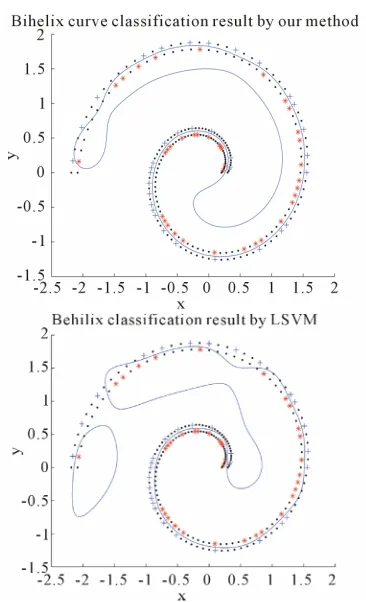
unlabeled data. The second one consists of 242 points taken from two nonlinear bihelix curves that are gene- rated by ab, where one is obtained by taking

0.2

a b , the other is by taking a0.2,b0.3,



0 :π 40 : 3π



[image:5.595.330.508.251.373.2]

 . We take randomly 30% of them as labeled and the remaining 70% as unlabeled. The com- parisons of our method with the LSVM method from [15] without the consideration of unlabeled data are given. Final results are illustrated in Figures 1 and 2.

Figure 1. Result on linear artificial data of LSVM and the new algorithm.

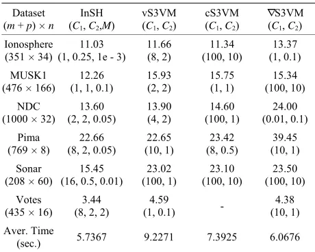
[image:5.595.330.513.407.708.2]

To reveal the efficiency of our algorithm for S3_VMs, comparisons of our algorithm (InSH) with some other existing algorithms for S3_{VMs such as the convex-} concave procedure in [5] (vS3_{VM), the continuation} method in [12] (cS3_{VM) and the gradient descent method} in [13] ( 3_{VM), are given for some standard test data} from [1 or the linear programming subproblem aris- ing in [5 we solve it with the Matlab function

[image:6.595.56.286.231.415.2]

in optim tion toolbox. The comparison ted in the following Table 1.

Table 1. Comparison Results on test data (test error %).

S

0]. F ], iza

linprog

results are lis-

Dataset (m + p) × n

InSH (C1, C2,M)

vS3VM (C1, C2)

cS3VM (C1, C2)

∇S3VM (C1, C2)

Ionosphere (351 × 34)

11.03 (1,0.25,1e - 3)

11.66 (8,2)

11.34 (100,10)

13.37 (1,0.1) MUSK1

(476 × 166)

12.26 (1,1,0.1)

15.93 (2,2)

15.75 (1,1)

15.34 (100,10) NDC

(1000 × 32)

13.60 (2,2,0.05)

13.90 (4,2)

14.60 (100,1)

24.00 (0.01,0.1) Pima

(769 × 8)

22.66 (8,2,0.05)

22.65 (10,1)

23.42 (8,0.5)

39.45 (10,1) Sonar

(208 × 60)

15.45 (16,0.5,0.01)

23.02 (100,1)

23.10 (100,10)

23.50 (100,10) Votes 3.44 4.59

(435 × 16) (8,2,2)

(1,0.1) -

4.38 (10, A

1) ver. Time _{5.7367 9.2271 7.3925 6.0676}

(sec.)

-: denotes the method fails for the

s rfor er

r s Mat on W s

Core 2 Du U 1 z

pr and ega f m

n e ,

dataset.

All the computation are pe med on a comput unning the

Vista with

oftware Intel(R)

lab 7.0 (TM)

Microsoft o CP

indow .83 GH ocessor

computatio

1789 m , we tak

bytes o 0 0.

emory. Du

1

m

h  ,

ring th

1e 3



e

1

h h   ,

1 1e 3

   , _N  1e 3, _c  1e 3,





3_{, 2}3_{ 1e}



, 2

C C_  _ 3,1e 2 , M



1e3,



cess e

2 are taken as th

kernel par

e one for the ameter

least test error. If ne ary, th

 is mo

taken th best leads toe the leas t test error a ng



1e



exact in

1,3 e

s a



n dex

. Th et are t k

para et en as

m ers for dete r-mining the i

 









2 ln max t



1

1 2

2 2

ln 2 1 max p, q,1 , 1.

t m t

 

4 1

,1 , 1;

,

t

x t



 m 

  



 _ 

   

 

  

 _{ }

  

  _{ }

 



where p2 1



t B



f ,









6 1 g f g 2 g

q t B B tB t B , B_f max



f₁i

 

x



and Bg max max



 

A



. 2

 

x t, has the same ex-

pression as 1

 

x t, where max



2

 

,



i f

B  f x t and

 





max max

g

B  B . ₁ and ₂ are taken as

1 2 1e 3

    th are given to bound the error of at

HH and DH .

5. Acknowledgements

DH

 

The research was supported by the National Nature Sci- ence Foundation of China (No. 11001092) and the Tian- Yuan Special Funds of the National Natural Science Foundation of China (Grant No. 11226304).

REFERENCES

[1] A. Astorino and A. Fuduli, “Nonsmooth Optimization Techniques for Semi- pervised

ons on alysis and Machine I gence, Vol. 29, No. 12, 2007, pp.

doi:10.1109

Su Classification,” IEEE Transacti Pattern An ntelli-

2135-2142. /TPAMI.2007.1102

“A Tutorial on Support Vector Machines , “

[2] C. J. C. Burges,

for Pattern Recognition Data Mining and Knowledge

998, pp. 121-167. 555

Discovery, Vol. 2, No. 2, 1 doi:10.1023/A:1009715923

[3] E. L. Allgower and K. Georg, “Numerical Continuation Methods: An Introduction,” Springer-Vergal, Berlin, 1990. doi:10.1007/978-3-642-61257-2

[4] E. Polak, J. O. Royset and R. S. Womersley, “Algorithms with Adaptive Smoothing for Finite Minimax Problems,”

Journal of Optimization Theory and Application, Vol.

119, No. 3, 20

doi:10.1023/B:JOTA.0000006685.60019.3e03, pp. 459-484.

[5] G. Fung and O. Mangasarian, “Semi-Supervised Support Vector Machines for Unlabeled Data Classification,” Op- timization Methods and Software, Vol. 15, No. 1, 2001,

pp. 29-44. doi:10.1080/10556780108805809

[6] G. X., Liu, “Aggregate Homotopy Methods for Solving Sequential Max-Min Problems, Complementarity Prob- lems and Variational Inequalities,” PhD Thesis, Jilin Uni- versity, Jilin, 2003.

[7] K. Bennett and A. Demiriz, “Semi-Supervised Support Vector Machines,” In: M. S. Kearns, S. A. Solla and D. A. Cohn, Eds, Advances in Neural Information Processing Systems, MIT Press, Vol. 10, 1998, pp. 368-374.

7, pp. 281- [8] L. T. Watson, S. C. Billups and A. P. Morgan, “Algo- rithm 652 Hompack: A Suite of Codes for Globally Con- vergent Homotopy Algorithms,” ACM Transactions on Mathematical Software, Vol. 13, No. 3, 198

310. doi:10.1145/29380.214343

[9] M. M. Mkela and P. Neittaanmki, “Nonsmooth Optimiza- tin: Analysis and Algorithms with Application to Optimal Control,” Utopia Press, Singapore, 1992.

[10] P. M. Murphy and D. W. Aha, “UCI Repository of Ma- chine Learning Databases.

http://www.ics.uci.edu/ mlearn/MLRepository.html. [11] O. Chapelle, V. Sindhwani and S. S. Keerthi, “Optimiza-

tion Techniques for Semi-Supervised Support Vector Machines,” Journal of Machine Learning Research, Vol. 9, 2008, pp. 203-233.

roceedings of the Tenth

i, “Branch and

stianini, “Semi-Supervised Learning

Regularization [13] O. Chapelle and A. Zien, “Semi-Supervised Classification

by Low Density Separation,” P

Scho

International Workshop on Artificial Intelligence and Sta- tistics, Vol. 1, 2005, pp. 57-64.

[14] O. Chapelle, V. Sindwani and S. Keerth

[18]

Bound for Semi-Supervised Support Vector Machines,”

Advances in Neural Information Processing Systems 19,

Proceedings of the 2006 Conference, MIT Press, Cam- M

bridge, 2007, pp. 217-224.

[15] O. L. Mangasarian and D. R. Musicant, “Lagrangian Sup- port Vector Machines,” Journal of Machine Learning Research, Vol. 1, 2001, pp. 161-177.

[16] S. Birbil, S. C. Fang and J. Han, “Entropic Regularization Approach for Mathematical Programs with Equilibrium Constraints,” Technical Report, Industrial Engineering and Operations Research, Carolina, 2002.

[17] T. D. Bie, N. Cri

Using Semi-Definite Programming,” In: O. Chapelle, B.

lkopf and A. Zien, Eds., Semi-Supervised Learning,

MIT Press, Cambridge, 2006.

X. J. Zhu, “Semi-Supervised Learning Literature Survey,” Technical Report 1530, Computer Science, University of Wisconsin-Madison, 2005.

[19] X. S. Li and S. C. Fang, “On the Entropic

ethod for Solving Min-Max Problems with Applica- tions,” Mathematical Methods and Operations Research,

Vol. 46, No. 1, 1997, pp. 119-130. doi:10.1007/BF01199466

[20] Y. Xiao, H. J. Xiong and B. Yu, “Truncated Aggregate Homotopy Method for Nonconvex Nonlinear Program- ming,” Optimization Methods and Software, 2012, pp. 1-

ontrol Engineering,

18.

[21] H. J. Xiong and B. Yu, “Aggregate Homotopy Method for Semi-Supervised SVMs,” 2011 International Confer- ence on Electric Information and C