Retail forecasting: research and practice

1. [email protected] 2. [email protected] 3. [email protected]

Management Science

Working Paper 2018:04

Retail forecasting: research and practice

Robert Fildes, Lancaster Centre for Marketing Analytics and

Forecasting, Lancaster University Management School, UK

Shaohui Ma, School of Business, Nanjing Audit University, China

Stephan Kolassa, SAP Switzerland

The Department of Management Science

Lancaster University Management School

Lancaster LA1 4YX

UK

© Robert Fildes, Shaohui Ma, Stephan Kolassa All rights reserved. Short sections of text, not to exceed two paragraphs, may be quoted without explicit permission,

provided that full acknowledgment is given.

LUMS home page: http://www.lums.lancs.ac.uk.

1. [email protected] 2. [email protected] 3. [email protected]

Retail forecasting: research and practice

Robert Fildes1_{, Lancaster Centre for Marketing Analytics and Forecasting} Department of Management Science, Lancaster University, LA1 1 Shaohui Ma2_{, School of Business, Nanjing Audit University, Nanjing, 211815, China}

Stephan Kolassa3_{, SAP Switzerland, SAP Switzerland} 8274 Tägerwilen, Switzerland

Abstract

This paper first introduces the forecasting problems faced by large retailers, from the strategic to the operational, from the store to the competing channels of distribution as sales are aggregated over products to brands to categories and to the company overall. Aggregated forecasting that supports strategic decisions is discussed on three levels: the aggregate retail sales in a market, in a chain, and in a store. Product level forecasts usually relate to operational decisions where the hierarchy of sales data across time, product and the supply chain is examined. Various characteristics and the influential factors which affect product level retail sales are discussed. The data rich environment at lower product hierarchies makes data pooling an often appropriate strategy to improve forecasts, but success depends on the data characteristics and common factors influencing sales and potential demand. Marketing mix and promotions pose an important challenge, both to the researcher and the practicing forecaster. Online review information too adds further complexity so that forecasters potentially face a dimensionality problem of too many variables and too little data. The paper goes on to examine evidence on the alternative methods used to forecast product sales and their comparative forecasting accuracy. Many of the complex methods proposed have provided very little evidence to convince as to their value, which poses further research questions. In contrast, some ambitious econometric methods have been shown to outperform all the simpler alternatives including those used in practice. New product forecasting methods are examined separately where limited evidence is available as to how effective the various approaches are. The paper concludes with some evidence describing company forecasting practice, offering conclusions as to the research gaps but also the barriers to improved practice.

1

1.

Introduction

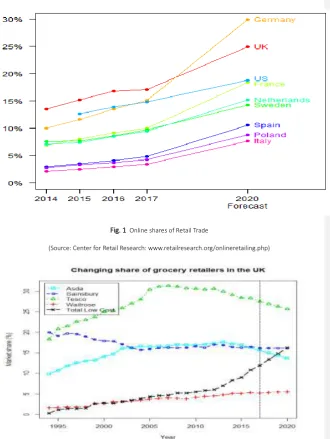
The retail industry is experiencing rapid developments both in structure, with the growth in on-line business, and in the competitive environment which companies are facing. There is no simple story that transcends national boundaries, with different national consumers behaving in very different ways. For example, in 2017 on-line retailing accounted for 14.8 % of retail sales in the US, 17.6% in the UK but only 3.4% in Italy contrasting with Germany showing a 3.5% increase to 15.1% since 2015 (www.retailresearch.org/onlineretailing.php). But whatever the retailer’s problem, its solution will depend in part on demand forecasts, delivered through methods and processes embedded in a forecasting support system (FSS). High accuracy demand forecasting has an impact on organizational performance because it improves many features of the retail supply chain. At the organizational level, sales forecasts are essential inputs to many decision activities in functional areas such as marketing, sales, and production/purchasing, as well as finance and accounting. Sales forecasts also provide the basis for national, regional and local distribution and replenishment plans.

Much effort has been devoted over the past several decades to the development and improvement of forecasting models. In this paper we review the research as it applies to retail forecasting, drawing boundaries around the field to focus on food, non-food including electrical goods (but excluding for example, cars, petrol or telephony), and non-store sales (catalog and now internet). This broadly matches the definitions and categories adopted, for example, in the UK and US government retail statistics. Our objective is to draw together and critically evaluate a diverse research literature in the context of the practical decisions that retailers must make that depend on quantitative forecasts. In this examination we look at the variety of demand patterns in the different marketing contexts and levels of aggregation where forecasts must be made to support decisions, from the strategic to the operational. Perhaps surprisingly, given the importance of retail forecasting, we find the research literature is both limited and often fails to address the retailer’s decision context.

2

three considers aggregate forecasting from the market as a whole where, as we have noted, rapid changes are taking place, down to the individual store where again the question of where stores should be located has risen to prominence with the changes seen in shopping behavior. We next turn to more detailed Stock Keeping Unit (SKU) forecasting, and the hierarchies these SKUs naturally fall into. The data issues faced when forecasting include stock-outs, seasonality and calendar events while key demand drivers are the marketing mix and promotions. On-line product reviews and social media are new information sources that requires considerable care if they are to prove valuable in forecasting. Section 5 provides an evaluation of the different models used in product level demand forecasting in an attempt to provide definitive evidence as to the circumstances where more complex methods add value. New product forecasting requires different approaches and these are considered in Section 6. Practice varies dramatically across the retail sector, in part because of its diversity, and in Section 7 we provide various vignettes based on case observation which capture some of the issues retailers face and how they provide operational solutions. Finally, Section 8 contains our conclusions as to those areas where evidence is strong as to best practice and where research is most needed.

2.

Retailers’ forecasting needs

Strategic level

3

strategic threat on-line and low price retailers pose, exacerbated by a dominant player in Amazon.

Fig. 1 Online shares of Retail Trade

(Source: Center for Retail Research: www.retailresearch.org/onlineretailing.php)

Fig. 2 Share of grocery retailers compared to the low price retailers (Aldi and Lidl) in the UK, 1994 to 2017 with ETS

4

These figures and the extrapolative forecasts show the rapid changes in the retail environment which require companies to respond. For example, a channel decision to develop an on-line presence will depend on a forecast time horizon looking decades ahead but with some quantitative precision required over shorter horizons, perhaps as soon as its possible implementation a year or more ahead. The retailer chain’s chosen strategy will require decisions that respond to the above changes: on location including channels, price/quality position and target market segment(s), store type (in town vs megastores) and distribution network. A key point is that such decisions will all typically have long-term consequences with high costs incurred if subsequent changes are needed, flexibility being low (e.g. site location and the move to more frequent local shopping in the UK, away from the large out-of-town stores, leading Tesco in 2015 to sell 14 of its earmarked sites in the UK and close down others and, in 2018, M&S proposing to close down more than 10% of its stores). Strategic forecasts are therefore required at both at a highly aggregate level and also a geographic specific level over a long forecast horizon.

The small local retailer faces just as volatile an environment, with uncertainty as to the location and target market (and product mix). Some compete directly with national chains where the issue is what market share can be captured and sustained. But while many of the questions faced by the national retailers remain relevant (e.g. on-line offering) there is little in the research literature that is even descriptive of the results of the many small shop location decisions. Exceptions include charity shops (Alexander, Cryer, and Wood, 2008) and convenience stores (Wood and Browne, 2007) while a number of studies examine restaurants which are outside our scope. But in this article, we focus on larger retailers carrying a wide range of products.

Tactical level

5

At the category level the objective again is to maximize category (rather than brand) profits which will require a pricing/ promotional plan that determines such aspects as the number and depth of promotions over the planning horizon (of perhaps a year), their frequency, and whether there are associated display and feature advertising campaigns. These plans are in principle linked to operational promotional pricing decisions discussed below. The on-shelf availability of products is also a key metric of retail service, and this depends crucially on establishing a relationship between the product demand forecasts, inventory investment and the distribution system. The range of products listed raises the question of new product introduction into a category, the expected sales and its effect on sales overall (particularly within category).

Demands placed on the warehouse and distribution system by store × product demand also need forecasting. This is needed to plan the workforce where the number and ‘size’ of products determines the pick rate which in turn determines the workforce and its schedule. The constitution of the delivery fleet and planned routes similarly depend on store demand forecasts (somewhat disaggregated) since seasonal patterns of purchasing vary by region. This is true whether the retailer runs its own distribution network or has it outsourced to a service provider – or, what is most common, uses a mixture, with many products supplied from the retailer’s own distribution centers, but others supplied directly by manufacturers to stores (Direct Store Delivery).

Operational level

6 distribution.

As a result of these various operational decisions with their financial consequences, the cash retailers generate (since suppliers are usually paid in arrears) leads to a cash management investment problem. Thus the cash available for investment, itself dependent on the customer payment arrangements, needs to be forecast.

Day-to-day store operations are also forecast dependent. In particular, staffing schedules depend on anticipated customer activity and product intake.

3.

Aggregate retail sales forecasting

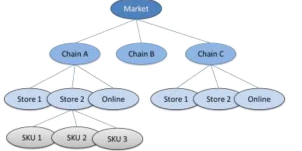
All forecasting in retail depends on a degree of aggregation. The aggregations could be on product units, location or time buckets or promotion according to the objective of the forecasting activity.

Fig. 3 Hierarchy of aggregate retail sales forecasting

7

store. Though forecasting aggregate sales at these three levels share many common issues, e.g., seasonality and trend, they raise different forecasting questions; have different objectives, data characteristics, and solutions.

3.1 Market level aggregate sales forecasting

Market level aggregate sales forecasting concerns the forecasts of total sales of a retail format, section, or the whole industry in a country or region. The time bucket for the market level forecasts may be monthly, quarterly or yearly. The forecasts of market level retail sales are necessary for (large) retailers both to understand changing market conditions and how these affect their own total sales (Alon, Qi, and Sadowski, 2001). They are also central to the planning and operation of a retail business at the strategic chain level in that they help identify the growth potential of different business modes and stimulate the development of new strategies to maintain market position.

Market level aggregate retail sales data often exhibit strong trend, seasonal variations, serial correlation and regime shifts because any long span in the data may include both economic growth, inflation and unexpected events (Fig. 4). Time series models have provided a solution to capturing these stylized characteristics. Thus, time series models have long been applied for market level aggregate retail sales forecasting (e.g., Alon et al., 2001; Bechter and Rutner, 1978; Schmidt, 1979; Zhang and Qi, 2005). Simple exponential smoothing and its extensions to include trend and seasonal (Holt-Winters), and ARIMA models have been the most frequent time series models employed for market level sales forecasting. Even in the earliest references, reflecting controversies in the macroeconomic literature, the researchers raised the question of which of various time series models performed best and how they compared with simple econometric models1 _{. The early studies suffered from a common}

weakness – a failure to compare models convincingly.

1 _{Typically, macro econometric models do not include retail sales as an endogenous variable but rather use a}

8

Fig. 4 US retail sales monthly series in million dollars.

(Source: U.S. Census Bureau)

Some researchers found that standard time series models were sometimes inadequate to approximate aggregate retail sales, identifying evidence of nonlinearity and volatility in the market level retail sales time series. Thus, researchers have resorted to nonlinear models, especially artificial neural networks (Alon, et al., 2001; Chu and Zhang, 2003; Zhang and Qi, 2005). Results have indicated that traditional time series models with stochastic trend, such as Winters exponential smoothing and ARIMA, performed well when macroeconomic conditions were relatively stable. When economic conditions were volatile (with rapid changes in economic conditions) ANNs was claimed to outperform the linear methods (Alon et al., 2001) though there must be a suspicion of overfitting. One study also found that prior seasonal adjustment of the data can significantly improve forecasting performance of the neural network model in forecasting market level aggregate retail sales (Kuvulmaz, Usanmaz, and Engin, 2005) although in wider NN research this conclusion is moot. Despite these claims this evidence of the forecasting benefits of non-linear models seems weak as we see below.

Econometric models depend on the successful identification of predictable explanatory variables compared to the time series model. Bechter and Rutner (1978) compared the forecasting performance of ARIMA and econometric models designed for US retail sales. They used two explanatory variables in the economic model: personal income and nonfinancial

Time

U

S

m

on

th

ly

re

ta

il

1995 2000 2005 2010 2015

150000

200000

250000

9

personal wealth as measured by an index of the price of common stocks; past values of retail sales were also included in alternative models that mixed autoregressive and economic components. They found that ARIMA forecasts were usually no better and often worse than forecasts generated by a simple single-equation economic model, and the mixed model had a better record over the entire 30-month forecast period than any of the other three models. No ex ante unconditional forecast comparisons have been found. Recently, Aye, Balcilar, Gupta, and Majumdar (2015) conducted a comprehensive comparative study over 26 (23 single and 3 combination) time series models to forecast South Africa's aggregate retail sales. Unlike the previous literature on retail sales forecasting, they not only looked at a wide array of linear and nonlinear models, but also generated multi-step-ahead forecasts using a real-time recursive estimation scheme over the out-of-sample period. In addition, they considered loss functions that overweight the forecast error in booms and recessions. They found that no unique model performed the best across all scenarios. However, combination forecast models, especially the discounted mean-square forecast error method (Stock and Watson, 2010) which weights current information more than past, not only produced better forecasts, but were also largely unaffected by business cycles and time horizons.

In summary, no research has been found that uses current econometric methods to link retail sales to macroeconomic variables such as GDP and evaluate their conditional and unconditional performance compared to time series approaches. The evidence on the performance of non-linear models is limited with too few series from too few countries and the comparison with econometric models has not been made.

3.2 Chain level aggregate sales forecasting

Research at the retail chain level has mainly focused on sales forecasting one year-ahead (Curtis, Lundholm, and McVay, 2014; Kesavan, Gaur, and Raman, 2010; Osadchiy, Gaur, and Seshadri, 2013). Accurate forecasts of chain level retail sales (in money terms) are needed for company financial management and also to aid financial investment decisions in the stocks of retail chains.

10

level forecasting (i.e. univariate extrapolation models). However, there are some specially designed models which have been found to have better performance. Kesavan et al. (2010) found that inventory and gross margin data can improve forecasting of annual sales at the chain level in the context of U.S. publicly quoted retailers. They incorporated cost of goods sold, inventory, and gross margin (the ratio of sales to cost of goods sold) as endogenous variables in a simultaneous equations model, and showed sales forecasts from this model to be more accurate than consensus forecasts from equity analysts. Osadchiy et al. (2013) presented a (highly structured) model to incorporate lagged financial market returns as well as financial analysts’ forecasts in forecasting firm-level sales for retailers. Their testing indicated that their method improved upon the accuracy of forecasts generated by equity analysts or time-series methods. Their use of benchmark methods (in particular a more standard econometric formulation) was limited. Building on earlier research Curtis et al. (2014) forecast retail chain sales using publicly available data on the age mix of stores in a retail chain. By distinguishing between growth in sales-generating units (i.e., new stores) and growth in sales per unit (i.e., comparable store growth rates), their forecasts proved significantly more accurate than the forecasts from models based on estimated rates of mean reversion in total sales as well as analysts’ forecasts. Internal models of chain sales forecasts should benefit from including additional confidential variables but no evidence has been found.

3.3 Store level aggregate sales forecasting

Retailers typically have multiple stores of different formats, serving different customer segments in different locations. Store sales are dramatically impacted by location, the local economy and competitive retailers, consumer demographics, own or competitor promotions, weather, seasons and local events including for example, festivals. Forecasting store sales can be classified into two categories: (1) forecasting existing store sales for distribution, target setting and viability, and financial control, and (2) forecasting new store potential sales for site selection analysis.

11

Davies (1973) used principal components and factor analysis in a clothing-chain study and demonstrated how the scores of individual stores on a set of factors may be interpreted to explain their sales performance levels. Geurts and Kelly (1986) presented a case study of forecasting department store monthly sales. They considered various factors in their test models including seasonality, holiday, number of weekend days, local consumer price index, average weekly earnings, and unemployment rate, etc. They concluded that univariate time series methods were better than judgment or econometric models at forecasting store sales. At a more operational level of managing staffing levels, Lam, Vandenbosch, and Pearce (1998) built a regression model based on daily data which set store sales potential as a function of store traffic volume, customer type, and customer response to sale force availability: the errors are modelled as ARIMA processes. However, no convincing evidence was presented on comparative accuracy. With the rapid changes on the high-street in many countries showing increasing vacancy rates, these forecasting models will increasingly have a new use: to identify shops to be closed. We speculate that multivariate time series models including indicator variables (for the store type), supplemented by local knowledge, should prove useful. But this is research still to be done.

Forecasting new store sales potential has been a difficult task, but crucial for the success of every retailing company. Traditionally, new store sales forecasting approaches could be classified into three categories: judgmental, analogue regression and space interaction models (also called gravitational models). Note that any evaluation of new store forecasts needs to take a potential selection bias into account: candidate new stores with higher forecasts are more likely to be developed and may see systematically lower sales than forecasted because of regression to the mean. (The analogue is also true for forecasting new product sales or promotional sales, see below.)

12

but is unable to predict turnover. The basic checklist approach can be further developed to emphasize “some variable points rating” to factors specific to success in particular sectors, for example, convenience store retailing (Hernandez and Bennison, 2000).

The analogue regression generates turnover forecasts for a new store by comparing the proposed site with existing analogous sites, measuring features such as competition (number of competitors, distance to key competitor, etc.), trading area composition (population size, average income, the number of households, commute patterns, car ownership, etc.), store accessibility (cost of parking, distance to parking, distance to bus station, etc.) and store characteristics (size, format, brand image, product range, opening hours, etc.). Compared with the judgmental approach, analogue regression models provide a more objective basis for the manager's decision-making, highlighting the most likely options for new locations. Simkin (1989) reported the success application of a regression based Store Location Assessment Model (SLAM) in several of the UK's major retailers. The model was able to account for approximately 80% of the store turnover, but prediction accuracy for the sales of new stores is not reported in the paper. Morphet (1991) applied regression to an analysis of the trading performance of a chain of grocery stores in the England incorporating five competitive and demographic factors (including population, share of floor space, distance higher order centre, pull, percentage of married women, etc.). Though the models achieved a high degree of 'explanation' of the variation in store performance, the results on predicted turnover suggested that the use of regression equations was insufficient to predict the potential performance of stores in new locations. The pitfalls of regressions may come from statistical overfitting due to limited data, neglecting consumer perceptions, and inadequate coverage of competition. While the method can include various demographic variables and is therefore appropriate for retail operations aiming for a segmented market it is heavily data dependent and therefore of limited value for a rapidly changing retail environment (as in the UK).

13

of SIM for location planning. Different from analogous regressions which mainly rely on the data from existing stores in the same chain, SIM uses data from various sources to improve prediction accuracy: analogous stores, household surveys, geographical information systems, competition and census data. A spatial interaction model is based on the theory that expenditure flows and subsequent store revenue are driven by the store’s potential attractiveness and constrained by distance, with consumers exhibiting a greater likelihood to shop at stores that are geographically proximate (Newing, Clarke, and Clarke, 2014). The basic example of this type of model is the Huff trade area model (Huff, 1963). Its popularity and longevity can be attributed to its conceptual appeal, relative ease of use, and applicability to a wide range of problems, of which predicting consumer spatial behavior is the most commonly known (Li and Liu, 2012). The original Huff model has been extended by adding additional components to make the model more realistic; these include models that can take into account retail chain image (Stanley and Sewall, 1976), asymmetric competition in retail store formats (Benito, Gallego, and Kopalle, 2004), store agglomeration effects (Li and Liu, 2012; Picone, Ridley, and Zandbergen, 2009; Teller and Reutterer, 2008), retail chain internal cannibalization (Beule, Poel, and Weghe, 2014), and consumer heterogeneity (Newing, et al., 2014). Furthermore, spatial data mining techniques and GIS simulation have been applied in retail location planning. These new techniques have proved to outperform the traditional modeling approach with regard to predictive accuracy (Lv, Bai, Yin, and Dong, 2008; Merino and Ramirez-Nafarrate, 2016).

Following Newing et al. (2014), let Sij represent the expenditure flowing between zone i and store j then

exp( )

exp( )

j ij

ij i

j ij

j

W C

S O

W C









14

that the model can be operationalized with a forecasting accuracy of around 10% (which proved better than the company’s performance). An important omission is the time horizon over which the model is assumed to apply, presumably the time horizon of the investment. Birkin et al. (2010) comment the models are regularly updated at least annually which suggests an implicit view as to lack of longer-term stability in the models arising from a changing retail environment. Extensions to the model suffer from problems of data inadequacies but Newing et al. (2014) argue these can be overcome to include more sophisticated demand terms such as seasonal fluctuation，and different types of retail consumer with different shopping behaviors.

Predictive models of store performance are only one element in supporting the location decision. Wood and Reynolds (2013) discuss how the models are combined with context specific knowledge and the judgments of location analysts and analogous information to produce final recommendations. There is no evidence available on the relative importance of judgmental inputs and model based information. Nor is there much evidence on the accuracy of the models beyond untested claims as to the model based forecasts being highly accurate (Wood and Reynolds, 2013) apart from Birkin et al.’s (2010) analysis of a DIY chain. In the rapidly changing retail environment, we speculate that judgment will again become the dominant approach to evaluating store potential and store closures. The research question now becomes what role if any models can usefully play.

Short-term forecasting of store activity can utilize recently available ‘big’ data in the form of customer credit (or mobile) transactions to produce shop sales forecasts. The use of the forecasts a week or so ahead is in staff scheduling. Ma and Fildes (2018) used mobile sales transactions, aggregated to daily store level for 2000 shops registered on a leading third-party mobile payment platform in China to show that the forecasts which took into account the overall activity on the platform (i.e. a multivariate approach) produced using a machine learning algorithm, outperformed univariate methods including standard benchmarks.

4.

Product level demand forecasting in retail

15

only one or a few of time series at a more aggregate level. The ability to accurately forecast the demand for each item sold in each retail store is critical to the survival and growth of a retail chain because many operational decisions such as pricing, space allocation, availability, ordering and inventory management for an item are directly related to its demand forecast. Order decisions need to ensure that the inventory level is not too high, to avoid high inventory costs, and not too low to avoid stock out and lost sales.

4.1 The hierarchical structure of product level demand forecasting

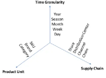
In general, given a decision-making question, we then need to characterize the product demand forecasting question on three dimensions: the level in the product hierarchy, the position in the retail supply chain, and the time granularity (Fig. 5): these are sometimes labelled ‘data cubes’..

Fig. 5 Multidimensional hierarchies in retail forecasting

Time granularity

16

promotion planning, and (initial) allocation planning, while on-line fashion sales may rely on an initial estimate of total seasonal sales, updated just once mid-season.

Product aggregation level

Three levels of the product hierarchy are often used for planning by retailers: SKU level, brand level, and category level.

SKU is the smallest unit for forecasting in retail, which is the basic operational unit for planning daily stock replenishment, distribution and, promotion. SKU level forecasts are usually conducted across stores up to the chain as a whole and in daily/weekly time steps. The number of SKUs in a retail chain may well be huge. E.g., in a supermarket, drugstore or home improvement/do it yourself (DIY) retailer today, tens thousands of items need weekly or even daily forecasts. Walmart faces the problem of over one billion SKU × Store combinations (Seaman, 2018). In a fashion chain such as Zara the number of in-store items by design, colour and size can also be of the order of tens of thousands, although forecasting may be conducted at the “style” or design level, aggregating historical data across sizes and colours and disaggregating using size curves and proportions to arrive at the final SKU forecasts. Online assortments are typically far larger, especially in the fashion, DIY or media (books, music, movies) business.

A brand in a product category often includes many variant SKUs with different package types, sizes, colors, or flavors. In addition to SKU level promotional planning, brand level forecasts are also important where there are cross-brand effects and promotions and ordering may be organized by brand.

17

by so-called category managers, who make large scale budgeting, planning and purchasing decisions, which again need to harmonize with the resources needed to actually execute these decisions, e.g., shelf space, planograms or specialized infrastructure like available freezer space.

Category management and the assortment decision starts with a category forecast which Kök, Fisher, and Vaidyanathan (2015) suggest is based on trend analysis supplemented by judgment. The assortment decision on which brands (or SKUs) to exclude as well as which new products to add is dependent on the SKU level demand forecasts: the effects on aggregate category sales of the product mix depend on the cross-elasticities of the within category SKU level demand forecasts, with a long (12 month) time horizon. The associated shelf-allocation is, Borin and Farris (1995) claim, insensitive to SKU demand forecast errors.

In short, whatever the focus, SKU level forecasts as well as their associated own and cross-price elasticities are needed to support both operational and tactical decisions.

Supply Chain

18

Ferrier, 2014). Empirical evidence on successful retail implementation is limited though Smaros (2007) using case studies identified some of the barriers and how they might be overcome (Kaipia, Holmström, Småros, and Rajala, 2017).

4.2 Forecasting within a product hierarchy

Given a specific retail decision-making question, we first need to determine the aggregation level for the output of the sales forecasting process. A common option is to choose a consistent level of aggregation of data and analysis. For example, if one needs to produce demand forecasts at the SKU-weekly-DC level it might seem ‘‘natural’’ to aggregate sales data to the SKU-weekly-DC level and analyze them at the same level as well. However, the forecasts can also be made by two additional forecasting processes within the data hierarchy: (1) the bottom-up forecasting process and (2) the top-down forecasting process.

The choice of the appropriate level of aggregation depends on the underlying demand generation process. Existing researches have shown that the bottom-up approach is needed when there are large differences in structure across demand time series and underlying drivers (Orcutt and Edwards, 2010; Zellner and Tobias, 2000; Zotteri and Kalchschmidt, 2007; Zotteri, Kalchschmidt, and Caniato, 2005). This is particularly true when the demand time series are driven by item specific time-varied promotions. Foekens, Leeflang, and Wittink (1994) found that disaggregate models produce higher relative frequencies of statistically significant promotion effects with magnitudes in the expected ranges. However, in the case of many homogeneous demand series and small samples, the top-down approach can generate more accurate forecasts (Jin, Williams, Tokar, and Waller, 2015; Zotteri and Kalchschmidt, 2007; Zotteri et al., 2005). For instance, different brands of ice cream will have a similar seasonality with a summer peak, which may not be easily detected for low-volume flavors but can be estimated at a group level and applied on the product level (Syntetos, Babai, Boylan, Kolassa, and Nikolopoulos, 2016). Song (2015) suggested that it is beneficial to model and forecast at the level of data where stronger and more seasonal information can be collected.

19

2007). For example, when aggregating product category level demand over stores, one can cluster stores according to whether they have similar demand patterns rather than according to their geographical proximity. A priori clustering based on store characteristics such as size, range and location is common. Appropriately implemented clustering can enable the capture of differences among stores (e.g., in terms of price sensitivity) as the clustering procedure groups stores with similar demand patterns (e.g., with similar reaction to price changes). In these terms, clustering is capable of resolving the trade-off between aggregate parameterization and heterogeneity, leading towards more efficient solutions. But so far, the weight of contributions on this issue focused only on the use of aggregation to estimate seasonality factors (Chen and Boylan, 2007). These works provided evidence that aggregating correlated time series can be helpful to better estimate seasonality since it can reduce variability.

Hyndman, Ahmed, Athanasopoulos, and Shang (2011) proposed a method for optimally reconciling forecasts of all series in a hierarchy to ensure they add up consistently over the hierarchy levels. Forecasts on all-time series in the hierarchy are generated separately first and these separate forecasts are then combined using a linear transformation. So far the approach has not been examined for retail demand forecasting applications.

20

4.3 Product level retail sales data characteristics and the influential drivers of

demand

At the product level, many factors may affect the characteristics of the observed sales data and underlying demand. Some of the factors are within the control of retailers (such as pricing and promotions, and “secondary” effects like interaction or cannibalization effects from listed, delisted or promoted substitute or complementary products), other factors are not controllable, but their timing is known (such as sporting events, seasons and holidays), and some factors are themselves based on forecasts (such as the competition, local and national economy and weather). There are also many other unexpected drivers of retail sales, such as abnormal events (like terror attacks or health scares), which manifest themselves as random disturbances to sales time series which are correlated across category and stores that share common sensitive characteristics.

As the result of these diverse effects, product level sales data are characterized by high volatility and skewness, multiple seasonal cycles, their often large volume, intermittence with zero sales frequently observed at store level, together with high dimensionality in any explanatory variable space. In addition, the data are also contaminated by stock-outs where the consumer is unable to purchase the product desired and instead may shift to another brand or size or, in the extreme, leave to seek out a related competitor.

Stock-outs: demand vs. sales

21

observations. The methods can be classified into two categories: nonparametric (e.g., Kaplan and Meier,1958) and parametric models using hazard rate techniques (e.g., Wecker, 1978; Nahmias, 1994; Agrawal and Smith, 1996). For more detail, see Tan and Karabati (2004) who provided a review on the estimation of demand distributions with unobservable lost sales for inventory control. Most of methods are based on stock out events data, while Jain, Rudi, and Wang (2014) found that stock-out timing could further improve the estimation accuracy compared with methods based on stock-out events. In the marketing and assortment management literatures, researchers have focused on the consumers’ substitution seeking behavior when their target product is facing stock out, which is another way of viewing the problem of product availability (e.g., Kök and Fisher , 2007; Vulcano, Ryzin, and Ratliff , 2012; Conlon and Mortimer, 2013).

Conversely, there is some evidence that at least for some categories, demand depends on inventory, with higher inventory levels driving higher sales: this has been called a “billboard effect” (Koschat, 2008; Ton and Raman, 2010). Anecdotally, we have encountered retailers who know this putative effect as “product pressure”. However, no literature appears to have leveraged inventories as a driver to improve forecasts.

22

Intermittence

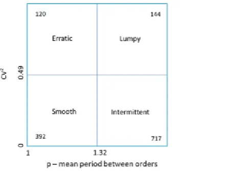
Intermittence is another common characteristic in store POS sales data, especially in slow moving items at daily SKU level. Fig.6depicts a SBC (Syntetos, Boylan, and Croston, 2005) categorization (see also Kostenko and Hyndman, 2006) over the daily sales of 1373 household cleaning items from a UK retailer, cross-classified by the coefficient of variation in demand and the mean period between non-zero sales. 861 items exhibit strong intermittent characteristics.

Fig. 6 SBC categorization on 1373 household clean items (Source: UK supermarket data)

23

benchmark –, Shenstone & Hyndman (2005) point out that any possible underlying model will be inconsistent with the properties of intermittent demands, exhibiting non-integer and/or negative demands. Nevertheless, Shenstone & Hyndman note that Croston’s point forecasts and prediction intervals may still be useful.

As mentioned in the stock-out discussion, POS sales are not the same as the latent demand. The observed zero sales may either be due to the product’s temporary unavailability (e.g., stock out or changes in assortment) or intermittent demand. Without product availability information, it is hard to infer the latent demand using only sales data. Much of the retail forecasting literatures when dealing with forecasting of slow moving items has not recognized this problem in their empirical studies (e.g., Cooper, Baron, Levy, Swisher, and Gogos, 1999; Li and Lim , 2018), while the only exception found is Seeger, Salinas, and Flunkert (2016) who treat demand in a stock-out period (assuming stock-out is observable) as latent in their Bayesian latent state model of on-line demand for Amazon products.

Product level demand in retail is also disturbed by a number of exogenous factors, such as promotions, special events, seasonalities and weather, etc. (as will be discussed in what follows): all of these factors make intermittent demand models difficult to be applied to POS sales data. One possibility is to model these influences on intermittent demands via Poisson or Negative Binomial regression. Kolassa (2016) found that the best models included only day of week patterns. One alternative approach, yet to be explored in retail, is the use of time series aggregation through MAPA (Kourentzes, Petropoulos, and Trapero, 2014) to overcome the intermittence, which then could be translated into distribution centre loading.

Seasonality

24

models with sufficient flexibility but parsimonious complexity to capture the seasonality of weekly retail data: trigonometric functions prove sufficient.

Fig. 7 Beer daily and weekly sales: UK supermarket data

Calendar events

Retail sales data are strongly affected by some calendar events. These events may include holidays (Fig. shows a significant lift in Christmas, i.e., week 51), festivals, and special activities (e.g., important sport matches or local activities). For example, Divakar, Ratchford, and Shankar (2005) found that during holidays the demand for beverages increased substantially, while other product groups were negatively affected. In addition, SKU × Store consumption may change due to changes in the localized temporary demographics. Most research includes dummy variables for the main holidays in their regression models (Cooper et al., 1999). Certain holidays recur at regular intervals and can thus be modeled as seasonality, e.g., Christmas or the Fourth of July in the US. Other holidays move around more or less widely in the (Western style) calendar and are therefore not be captured as seasonality, such as Easter, Labor Day in the US, or various religious holidays whose date is determined based on non-Western calendars, such as the Jewish or the Muslim lunar calendars.

Weather

25

higher when the weather is hot (e.g., Cooper et al., 1999; Dubé, 2004). Murray and Muro (2010) found that as exposure to sunlight increases, consumer spending tends to increase. Nikolopoulos and Fildes (2013) showed how a brewing company’s simple exponential smoothing method for in-house retail SKU sales could be adjusted (outside the base statistical forecasts) to take into account temperature effects.

Weather effects may well be non-linear. For instance, sales of soft drinks as a function of temperature will usually be flat for low to medium temperatures, then increase with hotter weather, but the increase may taper off with extreme heat, when people switch from sugary soft drinks to straight water. Such effects could in principle be modeled using spline transformations of temperature.

One challenge in using weather data to improve retail sales forecasts is that there is a plethora of weather variables available from weather data providers, from temperatures (mean temperature during a day, or maximum temperature, or measures in between) to the amount, duration and type of precipitation, or the sunshine duration, wind speed or wind chill factors, to even more obscure possibilities. One can either choose some of these variables to include in the model, or transform them in an appropriate way. For instance, one can define a Boolean “barbecue predictor”, which is TRUE whenever, say, the temperature exceeds 20 degrees Celsius and there is less than 20% cloud cover. In addition, there are interactions between the weather and other predictors, like promotions or the time of year: sunny weather will have a stronger impact on a promoted ice cream brand than on an unpromoted one, and “barbecue weather” will have a stronger impact on steak sales at the beginning of the summer, when people can observe “the first barbecue of the season”, than later in the year after they have been barbecuing for months.

26

forecasting appraisal overstate the forecast’s certainty, since they do not include the uncertainty inherent in the weather forecast. This uncertainty can in principle be surmounted in analyzes; however, it has been our experience that historical weather forecasts are much more expensive to obtain from data providers than historical actual weather data. Plus, one needs to ensure the correct vintage of forecasts: to calculate two-day-ahead sales forecasts, we need two-day-ahead weather forecasts, for three-day-ahead sales forecasts, we need three-day-ahead weather forecasts and so on.

Marketing mix and promotions

27

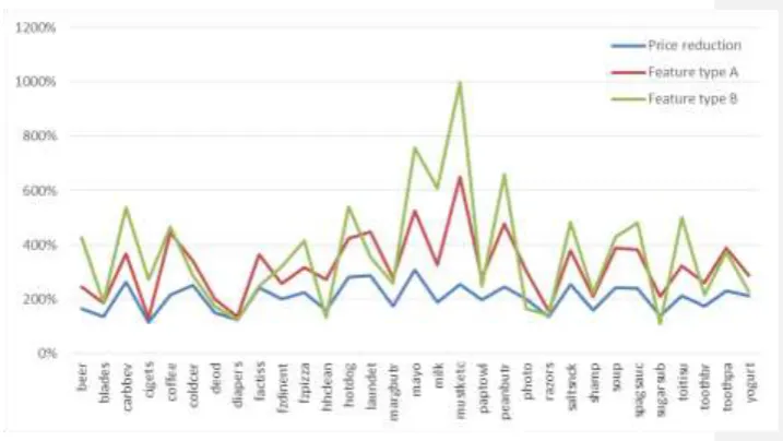
points or an additional coupon; to get the free unit, the shopper may need to buy one (“vanilla” BOGOF), two or more units; and the promotion may run for one day, one week, or multiple weeks (with typically declining impact); or it may be part of a larger advertising campaign like an “advent calendar”. The possible combinations will interact in different ways, and the quest for novelty on the part of retailer marketers ensures that products will regularly need to be forecasted with a marketing mix not previously observed for this particular product – necessitating a kind of “new promotion” forecasting analogous to a degree to new store and new product forecasting.

Fig. 8 Promotional lift effects in IRI dataset among various categories. Source: IRI data set.

28

signal at SKU × store level is strong enough to improve forecasts at this granular level and to actually improve the stock position on the shelf. In addition, modeling cannibalization requires a significant additional effort to identify drivers and victims, although product hierarchies may help here, and a retailer would likely restrict the modeling of cannibalization with its effort to important categories.

Finally, much the same discussion as for cannibalization applies to interaction effects from complementary products. For instance, a promotion on steaks may be hypothesized to increase the sales of steak sauces. The analysis of the two types of interaction – cannibalization and complementarity – differs in two key aspects. First, as noted above, product categories typically group similar products that are likely substitutes, so as noted above, the product category can be used to identify interacting pairs or groups of products. Conversely, the product hierarchy typically does not group complementary articles together, so it is not useful for identifying pairs or groups of products that may exhibit complementarity useful for forecasting. Second, however, basket analysis, i.e., the analysis of transaction log data with a view to which products were bought by the same shopper at the same time, can be useful in detecting complements, using affinity analysis – but basket analysis is harder to leverage to detect substitutes. However, cross-category price elasticities appear to be small, limiting the scope for improving forecasts using complementarity (Russell and Petersen, 2000). Ma, Fildes, and Huang (2016) show that improvements of 12.6% in forecasting accuracy (as measured by Mean Absolute Error) can be captured by the inclusion of competitive effects of 12% with cross-category effects of 0.6%.

29

Nikolopoulos, 2009) where one of the companies analyzed was a retailer. An important research issue is what if any benefits accrue from the increasingly complex alternative methods.

Online product reviews and social media

Online product reviews have been found to be an important source of market research information for online retailers in recent years (Floyd, Ling, Alhogail, Cho, and Freling, 2014) and we speculate this applies to all retailers where service is an important component. Since such reviews are a voluntary expression of consumers’ experiences and beliefs about the quality of products and services, consumers rely on online product reviews when making their own purchasing decisions (Chen and Xie, 2008; Zhao, Yang, Narayan, and Zhao, 2013). Researchers have found that there is a strong relationship between online word-of-mouth and product sales, but that the impact of word-of-mouth varies with product category (Archak, Ghose, and Ipeirotis, 2010; Chen, Wang, and Xie, 2011; Chevalier and Mayzlin, 2006; Hu, Koh, and Reddy, 2014; Zhu and Zhang, 2010). Thus, incorporating online product reviews, using tools such as text mining and sentiment analysis, may allow online retailers to add a new layer to their existing predictive models and boost predictive accuracy. However, it should be noted that fake reviews and so-called “sock puppetry” are a concern (Zhuang, Cui, and Peng, 2018) and automatically detecting such fake reviews is an active field of study (e.g., Kumar, Venugopal, Qiu, and Kumar (2018).

30

of predictors using, say, random projection (Schneider and Gupta, 2016). But on-line reviews, once measured, do not generate a uniquely important driver variable as they interact with any promotions, and both have proved important in forecasting in an application to Amazon on-line sales of electronic products (Chong, Li, Ngai, Ch'Ng, and Lee, 2016).

Similar challenges arise if we try to improve retail sales forecasts using social media data, such as Facebook, Twitter, Weibo, blogs or similar services. Here, a social media post first needs to be matched to the corresponding product – in the case of online product reviews on a product’s page, it is clear which product a review belongs to. Once this step is taken, similar text mining methods can be brought to bear on this topic as in the case of online product reviews. Care must be taken to distinguish forecasts using user-generated social media data from forecasts using social media data that the retailer (or the manufacturer) created in conducting marketing activities on social media (Kumar, Choi, and Greene, 2016) – both cases can be termed “forecasting with social media”, and confusion may result. Evangelos, Efthimios, and Konstantinos (2013) and Harald, et al. (2013) offer reviews on forecasting product sales (and other variables of interest) using social media data.

In either case, given the ephemerality of social media and the difficulty in forecasting customer reviews or social media posts themselves, in contrast to a retailer’s own marketing and pricing activities, these variables will likely only offer possibilities to improve short-term forecasts, not medium- or long-term ones. However, the evidence of success is extremely limited (Schaer, Kourentzes, and Fildes, 2018)

4.4 Data pooling

31

of different formats in diverse geographic regions. Pooling data across SKUs, subcategories and stores increases the size of the training dataset and the observed ranges for the explanatory variables. The marketing mix elasticities and seasonality patterns are usually assumed to be homogeneous in a pool of stores, but the baseline sales are allowed to be heterogeneous for different stores (Ainscough and Aronson, 1999; Baltas, 2005; van Donselaar, Peters, de Jong, and Broekmeulen, 2016). But the decision as to which variables should be assumed homogeneous (or heterogeneous) is still a matter of judgment. The downside of inappropriately assuming homogeneity is that the forecast equations are mis-specified with a resultant bias.

In the famous PromoCast model, Cooper et al. (1999) used a 67-variable cross-sectional pooled regression analysis of SKU-store sales under a variety of promotional conditions with store and chain specific historical performance information. Andrews, Currim, Leeflang, and Lim (2008) found that accommodating store-level heterogeneity does not improve the accuracy of marketing mix elasticities relative to the homogeneous model, and the improvements in fit and forecasting accuracy are also modest. Gür Ali, Sayin, van Woensel, and Fransoo (2009) compared the accuracy of 30 SKU sales prediction methods differing in data richness, technique complexity and model scope using a multi-store, multi-SKU European grocery sales database. They found that pooling observations across stores and subcategories provided better predictions than pooling across either only stores or only subcategories.

Contrasting with the findings by Andrews et al. (2008) and Gür Ali et al. (2009) that store homogeneous models provided better forecasts, Lang, Steiner, Weber, and Wechselberger (2015) found that allowing for heterogeneity in addition to functional flexibility (P-splines instead of linear) could improve the predictive performance of a store sales model considerably: incorporating heterogeneity alone only moderately improved or even decreased predictive validity.

32

(2015) present a pricing DSS for an online retailer, Rue La La, which offers extremely limited-time discounts (“flash sales”) on designer apparel and accessories. They used the features from the historical data to build a regression model for each product department, pooling data, starting with a SKU such as women’s athletic shoes to the top of the hierarchy, the department, such as footwear. The model then predicts demand of future first exposure styles depending on the price and level of discount as well as the SKU characteristics. While the forecast evaluation was cross-sectional, the successful revenue optimization experiment supported the effectiveness of the demand model.

In addition to data pooling, studies have also found that forecasts could be further improved by mining the residuals from many SKUs pooled across subcategories and stores. Based on the PromoCast model proposed by Cooper, et al. (1999), Cooper and Giuffrida (2000) use data mining techniques on the residuals to extract information from many-valued nominal variables, such as the manufacturer or merchandise category. The output of the data mining algorithm is a set of rules that specify what adjustments should be made to the forecast produced by the homogeneous market-response model. This combination means that a more complete array of information could be used to develop tactical planning forecasts. Trusov, Bodapati, and Cooper (2006) further improve the accuracy of the forecasts and interpretability of the recommendation system for promotional forecasts. Gür Ali and Pinar (2016) proposed a two-stage information sharing method. Segment-specific panel regressions with seasonality and marketing variables pool the data first; the residuals are then extrapolated non-parametrically using features that are constructed from the last twelve months of observations from the focal and related category-store time series. The forecast combines the extrapolated residuals with the forecasts from the first stage which showed out-of-sample accuracy improvements of 15%-30% over a horizon of 1 to 12 months compared with that of the one stage model. Exponential smoothing provided the benchmark where again the gains were substantial (of between 25%-40%).

33

use an individual model for that SKU or a pooled model considering all other SKUs? And how much historical data is enough? So far there is no systematic research to answer these questions.

4.5 Dimensionality reduction in presence of promotions

Any complete specification of the product (SKU) level determinants of store sales has high dimensionality in the explanatory variable space due to cross-item promotional interactions, which pose a big challenge in product demand forecasting. The model may be easily over-fitted or even cannot be estimated in this situation. The high dimensionality thus mainly stems from competing products within the same category (Ma et al., 2016).

One simple solution is to select the most influential subset of items in the same product category as the focal product. For example, the forecasting model named CHAN4CAST which was developed by Divakar et al. (2005) considers only the main competitor‘s promotional variables, i.e., considering only Pepsi’s promotions when forecasting the sales of Coca-Cola. Similarly, Lang et al. (2015) select the lowest price of a competing national (premium) brand in store as representative of the competition. Ma et al. (2016) used the promotional information from the top five sales products in the same category as the focal SKU, achieving a 6.7% improvement in forecast accuracy compared to models that only used information on the focal variable.

Another way of overcoming the dimensionality problem is to build predictive models based on summaries of the cross-promotional effects. The basic idea of this method is to build indexes which could summarize the cross promotional information. For example, van Donselaar et al. (2016) simply use the number of SKU in promotion as the summary of the promotional intensity in the category. Another straightforward way of building promotional indexes is to construct a weighted averaging of the promotion values (discount, display and feature) across SKUs in the category (e.g., Natter, Reutterer, Mild, and Taudes, 2007). Voleti, Kopalle, and Ghosh (2015) proposed a more elaborate approach by simultaneously incorporating branding hierarchy effects and inter-product similarity.

34

factor augmented regressions is that the factors are estimated without taking into account the dependent variable. Thus, when only a few factors are retained to represent the variations of the whole explanatory variable space, they might embody only limited predictive power for the dependent variable whereas the discarded factors might be useful.

Another solution is based on variable selection, especially by penalized likelihood method to automatically select influential promotion variables via continuous shrinkage (Gür Ali, 2013; Huang, et al., 2014; Ma, et al., 2016). Traditional best subset selection procedures are usually infeasible for high-dimensional data analysis because of the expensive computational cost. Penalized likelihood methods have been successfully developed over the last decades to cope with high dimensionality (Friedman, 2012; Tibshirani, 2011). A number of recent studies on product demand forecasting are all based on this method. For example, Gür Ali (2013) proposed a "Driver Moderator" method which uses basic SKU-store information and historical sales and promotion data to generate many features, and an L1-norm regularized regression simultaneously selects a few relevant features and estimates their parameters. Similarly, Huang et al. (2014) also identify the most relevant explanatory variables using L1-norm regularized methods. Ma et al. (2016) proposed a four step methodological framework which consists of the identification of potentially influential categories, the building of the explanatory variable space, variable selection and model estimation by a multistage LASSO (Least Absolute Shrinkage and Selection Operator) regression, followed by a scheme to generate forecasts. The success of this method for dealing with high dimensionality is demonstrated by substantial improvements in forecasting accuracy compared to alternative methods of simplifying the variable space. The multi-stage procedure overcomes the known limitation of LASSO for dealing with highly correlated explanatory variables.

35

potentially major benefits to be gained from estimating the loss from using simplified methods.

5.

Product level demand forecasting methods

Much effort has been devoted over the past several decades to the development and improvement of demand forecasting models in retail. Beyond well-established univariate extrapolative methods such as exponential smoothing, linear regression models (and variants) that include various driver variables are preferred over more complex models. Such linear models have the important practical advantage of easy interpretation and implementation. On the other hand, if linear models fail to perform well in both in-sample fitting and out-of-sample forecasting, more complex nonlinear models should be considered (Chu and Zhang, 2003). Indeed they are embedded in some commercial software (Fildes, Schaer, and Svetunkov, 2018). We here review these different classes of such models.

5.1 Univariate forecasting methods

36 5.2 Base-times-lift and judgmental adjustments

37

being the stated objective many of the adjustments were motivated by stocking/service level considerations. Some studies have shown that judgmental adjustments can enhance baseline forecasts during promotions, but not systematically: more advanced statistical models that include promotional indicators have proved better than the expert adjustments (Lim and O'Connor, 1996; Trapero, et al., 2014; Trapero, Pedregal, Fildes, and Kourentzes, 2013) but the evidence is from manufacturing. Judgmental adjustments are often applied in retailing as we discuss in Section 7, nevertheless the scale of retail forecasting necessitates a more selective approach when considering adjustments than that seen in manufacturing (typically <20% compared to around 70%). This naturally motivates the search for modeling methods that include promotional and other variables. No evidence has been collected from the field as to how the inclusion of such explanatory variables affects the adjustment process, but case vignette 1 in Section 7 demonstrates that the use of an econometric modelling approach does not preclude subsequent adjustment. Experimental evidence suggest adjustments can take into account causal information though they are (as expected) smaller than optimal (Lim and O'Connor, 1996; Sroginis, Fildes, and Kourentzes, 2018). The research issue here is whether software can be designed to ensure expert information is incorporated into the forecast (through demand planning meetings, for example), avoiding double counting and excluding the irrelevant cues which commonly are part of the forecasting support system (FSS) and the associated organizational process.

5.3 Econometric methods

Another stream of studies uses a model-based system to forecast product sales by directly taking into account promotional (and other) information. These methods are usually based on multiple linear regression models or more complex econometric models whose exogenous inputs correspond to seasonality, calendar events, weather conditions, price, and promotion features.

38

based on regression models with different specifications: multiplicative (log-log), exponential (semi-log) and log-reciprocal functional forms are the most widely used parametric specifications to represent nonlinearities in sales response to promotional instruments. A well-known example is the SCAN*PRO model and its extensions which decompose sales for a brand into own- and cross -brand effects of price, feature advertising, aisle displays, week effects, and store effects (Andrews, et al., 2008; Foekens, et al., 1994; Van Heerde, Leeflang, and Wittink, 2000, 2001). PromoCast is another well-known promotion-event forecasting model which was developed by Cooper et al. (1999). They used a static cross-sectional regression analysis of SKU-store sales under a variety of promotion conditions, with store and chain specific historical performance information. Divakar et al. (2005) also employed a dynamic regression model capturing the effects of such variables as past sales, trend, own and competitor prices and promotional variables, and seasonality.

In addition to linear regressions, more sophistical models that include complex error correlation structures have been proposed. Curry, Divakar, Mathur, and Whiteman (1995) proposed a Bayesian VAR model to forecast canned soup product sales at the brand level. The model included the sales, price, and advertisement of four competing brands as endogenous variables. Baltas (2005) proposed a panel regression model that admits store heterogeneity, periodic sales variation, chain-wide sales shocks, and sales dynamics. Recently, using the IRI data set (Bronnenberg et al., 2008), Huang et al (2014) and Ma et al. (2016) have developed Autoregressive Distributed Lag (ADL) models and evaluated them on SKU data for many categories and a number of stores with the latter study showing that a Lasso procedure could successfully take into account both intra-category promotional variables (12% improvement in MAE) and inter-category (worth a further 0.6%). Arunraj and Ahrens (2015) developed a seasonal autoregressive integrated moving average with external variables (SARIMAX) model to forecast the daily sales of bananas in a German retail store. Michis (2015) proposed a wavelet smoothing method to improve conditional forecasts generated from linear regression sales response models.

39 5.4 Nonlinear and machine learning methods

Nonlinear methods include traditional nonlinear regressions, non- or semi-parametric regressions, and fuzzy and machine learning algorithms. Compared to the linear regression models, nonlinear methods allow arbitrary non-linear approximation functions derived (learned) directly from the data and this increased generality improves the potential to provide more accurate forecasts (though with an increased danger of overfitting).

For grocery products, most published research found improvements in forecasting accuracy by using nonlinear models over linear regressions. The models used include Back Propagation Neural Networks (Aburto and Weber, 2007; Ainscough and Aronson, 1999), Fuzzy Neural Networks (Kuo, 2001); Regression Trees (Gür Ali et al., 2009), Gray relation analysis and multilayer functional link networks (Chen and Ou, 2009, 2011), a two level switching model selecting between a simple moving average and a non-linear predictor (e.g., k-nearest neighbor, decision trees) based on the characteristics of the time series (Žliobaitė, Bakker, and Pechenizkiy, 2012), Support Vector Machines (Gür Ali and Yaman, 2013; Pillo, Latorre, Lucidi, and Procacci, 2016), Wavelets Neural Networks (Veiga, Veiga, Puchalski, Coelho, and Tortato, 2016), and Bayesian P-splines (Lang et al., 2015). An exception where non-linearities led to poor performance is van Donselaar et al. (2016) who analyzed the impact of relative price discounts on product sales during a promotion but did not find conclusive evidence for the presence of threshold and/or saturation levels for price discounts for perishable products. Despite the hype, if non-linearities were commonplace and easy to identify we would expect to see more of such models used in practice.

40

system which they found to be more accurate than a traditional SARIMA model. But the standard gradient learning algorithm estimation such as Back Propagation (BP) NN is relatively more time-consuming. Extreme learning machines (ELM), which provide much faster learning speed, have been adopted in a number of fashion forecasting studies (Wong and Guo, 2010; Xia, Zhang, Weng, and Ye, 2012; Yu, Choi, and Hui, 2011). The experimental results have shown that the performance of the ELM is more effective than traditional BPNN models for fashion sales forecasting but their accuracy compared to BPNN is at best moot. When the historical data is limited, Grey model based methods are claimed to have better performance (Choi, et al., 2014; Xia and Wong, 2014), but the results need to be further validated based on a larger sample of series. Du, Leung, and Kwong (2015) proposed a Multi-Objective Optimization-based Neural Network (MOONN) model which they claimed to be superior to several of the above mentioned methods for the short-term replenishment forecasting problem.

The scalability of the nonlinear models is usually poor so dealing with real retail applications with tens of thousands of SKUs in hundreds of stores is impractical with current computational powers. The amount of training time required to build and maintain nonlinear forecasting models becomes a serious concern. The size of the pooled dataset and memory limitations also raise estimation problems (Gür Ali and Yaman, 2013). For these reasons, existing researchers who have tried to test the superiority of nonlinear models at product level usually work at very small scale (i.e., tens of items). We conclude the evidence for non-linearity generally leading to better forecasting accuracy is weak, the positive evidence probably arising from ‘publication bias’: The studies cited have many limitations and these are summarized in the next section.

5.5 Comparative evaluation