Validation of Image Compression Algorithms using
Neural Network
Nikhilesh Joshi
Research Scholar, Dept of Computer Engg
Thadomal Shahani Engineering College,
Bandra(W), Mumbai
Tanuja K. Sarode, PhD
Professor & Head, Dept of Computer Engg,
Thadomal Shahani Engineering College,
Bandra(W), Mumbai
ABSTRACT
We live in Digital Era where information is generated at rapid space. Images constitute a major part of information. It becomes essential to use image compression techniques in order to reduce storage space and transmission bandwidth. Image compression algorithm can be validated using Neural Network. In this paper various methods of Image compression such as BTC, DCT, DWT are optimized and Validate using neural network. This is achieved by comparing methods based on set of parameters. . The resultant compression metrics are calculated and visual quality of image is analyzed. Neural network implementation is done based on two different methods desired matrix and entropy based method. Experimental analysis shows 60 % reduction in storage space requirement and effective optimization using different methodology.
General Terms
Image Processing, Neural Networks
Keywords
Image Compression, Entropy, Block Truncation Coding, Discrete Cosine Transform(DCT) Discrete wavelet tranform(DWT, Image Quality Metrics, Neural Network, Back propogation.
1.
INTRODUCTION
Now a day‟s most of the information is in the form of Images. Images require large amount of space for storage and consumes more bandwidth during transmission. Image Compression plays a vital role in reducing the storage space requirement and helps to increase transmission ratio over network. A gray scale image that is 256 x 256 will have 65, 536 pixels to store and a typical 640 x 480 color image have nearly a million. Downloading of these files from internet can be very time consuming task. Image data comprise of a significant portion of the multimedia data and occupy the major portion of the communication bandwidth for multimedia transmission. The image compression technique most often used is transform coding. Transform coding is an image compression technique that first switches to the frequency domain, then does its compression. The transform coefficients should be decor related, to reduce redundancy and to have a maximum amount of information stored in the smallest space [1] [2].
Two fundamental components of compression are redundancy and irrelevancy.
Redundancies reduction aims at removing duplicate information from the signal source (image/video). Irrelevancy reduction omits parts of the signal that
will not be noticed by the signal receiver
In digital image compression, three basic data redundancies can be identified and exploited:
1. Coding redundancy 2. Inter pixel redundancy 3. Psycho visual redundancy
Data compression is achieved when one or more of these redundancies are reduced or eliminated.
Coding redundancy use shorter code words for the more common gray levels and longer code words for the less common gray levels. This is called Variable Length Coding. To reduce this redundancy from an image we go for the Huffman technique were we are assigning fewer bits to the more probable gray levels than to the less probable ones achieves data compression.
Inter pixel redundancy is directly related to the inter pixel correlations within an image. Because the value of any given pixel can be reasonable predicted from the value of its neighbors, the information carried by individual pixels is relatively small. Much of the visual contribution of a single pixel to an image is redundant; it could have been guessed on the basis of its neighbor‟s values
Psycho visual redundancy: Human perception of the information in an image normally does not involve quantitative analysis of every pixel or luminance value in the image. In general, an observer searches for distinguishing features such as edges or textural regions and mentally combines them into recognizable groupings. The brain then correlates these groupings with prior knowledge in order to complete the image interpretation process. Thus eye does not respond with equal sensitivity to all visual information. Certain information simply has less relative importance than other information in normal visual processing. This information is said to be psycho visually redundant. The elimination of psycho visually redundant data results in a loss of quantitative information.
The Organization of this paper is as follows. The Performance Measure are described in Section II, DCTBTC in section III, Experimental Analysis of DCTBTC in section IV, DWTDCT and its experimental analysis in section V, Neural network design and its different method, experimental result in section VI, Comparative study in section VII and Conclusion in Section VIII
2.
PERFORMANCE PARAMETER
against other image compression technique. The metrics for image quality can be broadly classified as Subjective and objective. Subjective Quality metrics is used to determine the quality of image by evaluation of images and viewers read images. In case of objective quality metrics some statistical indices are calculated to indicate image quality. After reviewing the literature it can be concluded that certain set of parameter are involved in research to be performed. Some of the parameter can be standard parameter while some of them may be applicable to few selected Compression algorithms. i) Compression Ratio (CR): The performance of image compression can be specified in terms of compression efficiency which is measured by the compression ratio or by the bit rate. Compression ratio is the ratio of the size to original image to the size of compressed image and bit rate.
CR =
size of original image
size of compressed Image
… … … (1)
The compression ratio and bit rate are related. Let b be the number of bits per pixel of the uncompressed image, CR the compression ratio, bit rate BR will be calculated as:
𝐵𝑅 =
𝑏𝐶𝑅
… … … (2)
ii)Peak Signal to Noise Ratio: It is commonly used as a measure of quality of reconstruction of lossy compression. It is attractive measure for loss of image quality due to simplicity and mathematical convenience. PSNR is qualitative measure based on mean square error (MSE) of the reconstructed image. MSE gives the difference between original image and the reconstructed image and is calculated as follows:
MSE=
1MN
y i ,j - x i , j
2 Nj=1 M i=1
The PSNR is the quality of the reconstructed image and calculated as the inverse of MSE. If the reconstructed image is close to the original image, MSE is small and PSNR take large value. PSNR is dimensionless and expressed in decibel calculated as follows:
PSNR= 10 log
L2
MSE
………..(4)
iii)Structural Similarity Index: It is method for measuring similarity between two images. It is full reference metrics which mean the measuring of image quality is based on initial uncompressed or distortion free image as reference. SSIM is designed to overcome the inconsistent human eye perception in the traditional method like PSNR. It is defined as the function of three components luminance, contrast and structure and each of this components is calculated separately using (5),(6) & (7) respectively. Luminance change
l x ,y = 2μxμy+𝑐1 𝜇𝑥2+𝜇𝑦2+𝑐1
… … … . . … … (5)
Contrast change, c x, y = 2σxσy+𝑐2
𝜎𝑥2+𝜎𝑦2+𝑐2
… … … . … . (6)
Structural Change, s x, y = σxy+c3
σx σy +c3
……….(7)
SSIM x, y =l x,y .c x,y .s x,y ………...(8)
where x represent the original image y represent the reconstructed image and
𝜇𝑥 = 𝑎𝑣𝑒𝑟𝑎𝑔𝑒 𝑜𝑓 𝑥 𝜇𝑦 = 𝑎𝑣𝑒𝑟𝑎𝑔𝑒 𝑜𝑓 𝑦
𝜎𝑥= 𝑣𝑎𝑟𝑖𝑎𝑛𝑐𝑒 𝑜𝑓 𝑥 𝜎𝑦 = 𝑣𝑎𝑟𝑖𝑎𝑛𝑐𝑒 𝑜𝑓 𝑦
𝜎𝑥𝑦 = 𝑐𝑜𝑣𝑎𝑟𝑖𝑎𝑛𝑐𝑒 𝑜𝑓 𝑥 𝑎𝑛𝑑 𝑦
𝑐1 𝑎𝑛𝑑 𝑐2𝑎𝑟𝑒 𝑡𝑤𝑜 𝑣𝑎𝑟𝑖𝑎𝑏𝑙𝑒𝑠 𝑡𝑤𝑜 𝑣𝑎𝑟𝑖𝑎𝑏𝑙𝑒𝑠 𝑡𝑜 𝑠𝑡𝑎𝑏𝑖𝑙𝑖𝑧𝑒 𝑡𝑒
𝑑𝑖𝑣𝑖𝑠𝑖𝑜𝑛 𝑤𝑖𝑡 𝑤𝑒𝑎𝑘 𝑑𝑒𝑛𝑜𝑚𝑖𝑛𝑎𝑡𝑜𝑟.
𝑐1= 𝑘1𝐿 2, 𝑐2= 𝑘2𝐿 2 𝑐3= 𝑐2
2 𝑘1= 0.001
𝑘2= 0.002 𝑏𝑦 𝑑𝑒𝑓𝑎𝑢𝑙𝑡 𝐿 𝑖𝑠 𝑑𝑦𝑛𝑎𝑚𝑖𝑐 𝑟𝑎𝑛𝑔𝑒 𝑜𝑓 𝑝𝑖𝑥𝑒𝑙 𝑣𝑎𝑙𝑢𝑒 The resultant SSIM Index is a decimal value between -1 and 1and in case of two identical sets of data value of SSIM is 1.
iv)Entropy: It is an important factor to estimate whether the digital image is basically same with the original image. Entropy can be calculated by standard function available in Mat Lab. E = entropy (I) returns E, a scalar value representing the entropy of gray scale image. Entropy is statistical measure of randomness that can be used to characterize the texture of the input image. It is defined as
𝐸 = −𝑠𝑢𝑚 (𝑝 ∗ log
2𝑝) … … … . . (9)
Where p contains the histogram counts returned from imhist. v) Edge Measurement (Edge): This type of quality measure can be obtained from𝐸𝑑𝑔𝑒 =
1𝑀𝑁
𝑄 𝑖, 𝑗 − 𝑄 𝑖, 𝑗
2 𝐽𝑗 =1 𝐼 𝑖=1
……….(10)
Where
𝑄 𝑖, 𝑗 𝑎𝑛𝑑 𝑄 𝑖, 𝑗
are edge gradients of the original and compressed image using a Sobel operator. The higher the Edge Measurement means the lower of image quality. We need to check for edge measurement parameter since it is observed that in case of BTC there is distortion at the edges.vi)Each image is Normalized by its root power, So the correlation measurement is defined as
𝐶
=
𝑓 𝑚, 𝑛 𝑓
(𝑚, 𝑛)
𝑁 𝑛=1 𝑀
𝑚 =1
𝑓
2𝑚, 𝑛
𝑁𝑓
2𝑚 , 𝑛
𝑛=1𝑀
𝑚 =1
𝑁 𝑛=1 𝑀
𝑚 =1
=
𝑥 𝑚, 𝑛 𝑥
(𝑚, 𝑛)
𝑁 𝑛=1 𝑀 𝑚 =1
𝑥
2𝑚, 𝑛
𝑁𝑥
2𝑚 , 𝑛
𝑛=1 𝑀
𝑚 =1
𝑁 𝑛=1 𝑀 𝑚 =1
… . . (11)
3.
DCT & DCTBTC
Block Truncation Coding is the simplest and fast lossy compression technique for gray scale images. The focus is on moment preservation quantization for block of pixels [2]. The input image is divided in to non-overlapping block of pixel sizes depending upon requirement, for example the block size can be 2, 4, and 8. Mean and standard deviation is calculated for BTC which is the basic step. Mean can be considered as the threshold of image. The reconstruction values are determined using mean and standard deviation. Next bit map of the block is derived based on value of threshold which is compressed or encoded image. The reconstructed values and bitmap is used to by the decoder to reconstruct the image. In the encoding process, BTC produce a bitmap, mean and standard deviation for each block. This method provides a good compression without much degradation on the reconstructed image. A closer look shows some artifacts like staircase effect near the edges. It‟s because of simplicity and easy implementation it has gained widely used. To improve the quality of reconstructed image and better compression efficiency several variant of BTC has been developed over period of time.
Absolute Moment Block Truncation Coding (AMBTC) [3] provides better image quality than image compression using BTC. AMBTC preserves higher mean and lower mean of each block and use this quantity to quantize output. Most important aspect is that AMBTC is faster compared to BTC. Cheng and Tsai [4] proposed algorithm for image compression which was based on application of moment preserving edge detection. The algorithm is faster and involves simple analytical formulae to compute the parameter of the edge feature in an image block. In accordance with human perceptual experience the reconstructed image has good quality. In other paper [5] the author proposed an edge based and mean based algorithm that produce good quality image at very low bit rates. In one of the paper the authors [6] [7] proposed an improved BTC image compression using Fuzzy Complement Edge Operator.
In Modified way of performing BTC using min-max quantizer (MBTC) method instead of using the mean and standard deviation, average value of the maximum, minimum and mean of the blocks of pixels is calculated [9]. Based on this value of quantization is done, so that the difference between the pixel values in each segment is much more reduced. By implementing this method the error between the pixel values of the original and the reconstructed image is decreased and an improved quality image will be generated by the decoding process with the same bit rate as that of the conventional BTC.
Earlier BTC algorithm was proposed, in which there was problem of staircase at edges in the reconstructed image. In the BTC algorithm different block are selected depending on requirement. For experimental purpose we will have N as block size which can be 2/4/8/16/32. Depending on the Block size mean and standard deviation is calculated. The compressed bit map is obtained by
𝐵 =
1 𝑤
𝑖> 𝜇
0 𝑤
𝑖≤ 𝜇
… … … . (14)
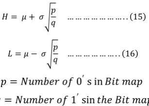
The bitmap B mean and standard deviation is transmitted at the decoder end. Next H and L are calculated as highlighted in equation 15 and 16 and reconstructed image can be obtained by replacing the element 1 in the B with H value and element 0 with L. The reconstructed highlighted in fig.1.In this process𝐻 = 𝜇 + 𝜎 𝑝
𝑞 … … … . . 15
𝐿 = 𝜇 − 𝜎 𝑝
𝑞 … … … . . 16
𝑝 = 𝑁𝑢𝑚𝑏𝑒𝑟 𝑜𝑓 0
′s in 𝐵𝑖𝑡 𝑚𝑎𝑝
𝑞 = 𝑁𝑢𝑚𝑏𝑒𝑟 𝑜𝑓 1
′sin 𝑡𝑒 𝐵𝑖𝑡 𝑚𝑎𝑝
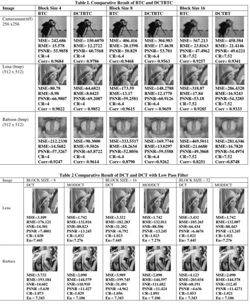
the parameters like MSE, PSNR, Correlation, CR are calculated and highlighted in table1. The image size varies from 512 x 512 and 256 x 256.(a) (b) (c) (d)
Fig.1 BTC Result (a) Original Image (256 x 256) (b) Reconstructed Image (4x4) (c) Reconstructed Image (8x8)
(d) Reconstructed Image(16 x16)
[image:3.595.352.506.71.180.2](a) b) (c) (d)
Fig.2 BTC Result (a) Original Image (256 x 256) (b) Reconstructed Image (4x4) (c) Reconstructed Image (8x8)
(d) Reconstructed Image(16 x16)
In the proposed algorithm which is termed as Discrete Cosine Transform Block code Truncation (DCTBTC), DCT is applied to the image and after that BTC is applied. One important change is that we first perform low pass filtering on the image and then DCTBTC is applied. In this way we can achieve a better image quality and correlation can be enhanced at the cost of MSE and PSNR which is tabulated in Table I. In terms of compression ratio the number of bits required to transmit the information can be reduced by considerably amount thus achieving better result. In the process we also calculate various Image quality parameters that where calculated in the previous BTC methodology [11][12]. The comparison is discussed in next section. DCT is the one of the simplest compression method that can be applied to an image. It is a popular transform used for some of the image compression standards in lossy compression methods. The disadvantage of using DCT image compression is the high loss of quality in compressed images, which is more notable at higher compression ratios. The discrete cosine transform (DCT) represents an image as a sum of sinusoids of varying magnitudes and frequencies. The DCT has the property that, for a typical image, most of the visually significant information about the image is concentrated in just a few coefficients of the DCT [16].
4.
EXPERIMENTAL ANALYSIS OF
DCTBTC
[image:3.595.312.542.172.405.2]performance of BTC and DCTBTC has been evaluated for set of standard images like Lena512, lena256, Baboon 512, Baboon256, Barbara512, Barbara256. Table I highlights the Comparative result of BTC and DCTBTC. The performance is measured based on quality metrics.
From the table I it can observe that the performance of proposed algorithm is better in terms of image quality. This can be concluded based on the parameter that were calculated for calculated for each of the images. DCTBTC, PSNR and MSE values are higher compared to the BTC methodology. It indicate enhancement in the visual quality of constructed image. The Compression ratio is most important aspect of compression. In BTC we use Block of different size. This helps in reducing the number of bits required for transmission. Hence 1 pixel require 8 bit for representation. If we have 256x256 images and block size 4x4 then the number of bits required is 524288 bits. In Compressed form it is represent by 0 or 1 so only 1 bit is required so 4x4 block require 16 bit representation and L and H which is transmitted require 16 bits so only 32 bits are required. In this way the total bits required for transmission in compressed form will be 64x64x32 = 131072 bits. So it can observed that transmission require less number of bits which result in less requirement of bandwidth and reduce storage space. The compression ratio can be calculated as given by equation (1) here it comes out to be 4 which is 25% compression can be achieved by this method.
In some of the images where the edges are not distinct because of inherent blurriness of pixel values due to nature of the images the edge position may or may not be accurate. This is reflected in the BTC reconstructed image. In DCTBTC since DCT is performed first and then BTC is applied the above problem is rectified to large extent. So the visual quality of image even at the edges is enhanced which can be clear from cameraman image as shown in Table 1. From the table it is clear that the staircase effect introduce by BTC at edges is reduced in DCTBCT. The Different Block size for same images also reflects the concept of reduction in raggedness of image quality at the edges.
5.
DWTDCT & EXPERIMENTAL
ANALYSIS
The discrete cosine transform (DCT) represents an image as a sum of sinusoids of varying magnitudes and frequencies. The DCT has the property that, for a typical image, most of the visually significant information is concentrated in just a few coefficients of the DCT. The DCT works by separating images into the parts of different frequencies. During a step called Quantization, where parts of compression actually occur, the less important frequencies are discarded. Then the most important frequencies that remain are used to retrieve the image in decomposition process. As a result, reconstructed image is distorted [17].
All mainstream encoders use the Discrete Cosine Transform (DCT) to perform transform coding that maps a time domain signals to a frequency domain representation. The frequency domain spectrum can be compressed by truncating low intensity regions. However, the DCT has drawbacks like computation takes long time and grows exponentially with signal size. If we want to calculate the DCT of entire video frame it will require unacceptable amount of time. The Solution is to partition video into small blocks and applies DCT to each partition which may lead to degradation of picture quality. The Discrete Wavelet Transform offers a
better solution. DWT is another transform that maps time domain signals to frequency domain representations. The DWT can be computed by performing a set of digital filters which can be done quickly. This allows us to apply the DWT on entire signals without taking a significant performance hit. By analyzing the entire signal the DWT captures more information than the DCT and can produce better results. The DWT separates the image‟s high frequency components from the rest of the image, resizes the remaining parts and rearranges them to form a new „transformed‟ image [17].
Method 1 (DCT Low pass)
Step 1: Load the image to be compressed.
Step 2: Decompress the image planes using DCT and Specific Block Size.
Step 3: Reconstruct the image using iDCT
Step 4: Apply Low Pass Filtering to smoothen the edges. Step 5: Save the compressed image and calculate Compression
Method 2 (DWT DCT Method)
Step 1: Load the image to be compressed.
Step 2: Split the original image to Y, Cb and Cr color
planes.
Step 3: Decompress the image planes using DWT. Step 4: Apply Sub band coding and shift data to create zero matrix.
Step 5: Create the transform array using DCT and Eliminate the zero matrixes using block N x N. Step6: Reconstruct the image using iDCT
Step 7: Save the compressed image and calculate Compression
The performance of both the method was evaluated and tabulated as shown in Table 2 and Table 3. Table 2 highlights the DCT method and DCT with low pass filter applied to compressed image along with performance parameters. Some set of standard images along with other format are considered. Table 3 highlights the DWT DCT methodology applied to the set of test images. Table 4 highlights the Correlation and Entropy for the set of images used. Table 5 highlights the result when DCT DWT is used for optimization of compression ratio.
Table 2 shows the result for Method 1 and parameters calculated for same. The various block size consider are represented in the table. Initially DCT is applied to original image and result reflects blurring effect or step at edges. To remove this effect low pass filtering is applied. It is observed that the quality of image has improved. Moreover in DCT methodology it is known that it follows zig- zag pattern for reduction. The image pixels are reduced to half while the process is being applied. Compression ratio indicates that image is compressed to substantial ratio and quality is also maintained. This helps in reducing storage space.
Table 3 shows the result of method 2. We apply DWT to original image of size 256 x 256, so it has 65536 pixel values. After applying the DWT we consider LL region of DWT which is 128 x 128 hence it has 16384 pixel values. DCT is applied to this and image is reconstructed. It is found that it reduces the storage space for images by more than 50% and helps in reducing the transmission bandwidth requirement.
Table I. Comparative Result of BTC and DCTBTC
Image Block Size 4 Block Size 8 Block Size 16
BTC DCTBTC BTC DCTBTC BTC DCTBT
Cameraman(tiff) 256 x256 MSE=242.686 RME=15.578 PSNR=55.9858 CR=4 Corr= 0.9684 MSE=150.6070 RME=12.2722 PSNR=60.7568 CR=4 Corr= 0.9786 MSE=406.416 RME=20.1598 PSNR=50.829 CR=6.4 Corr=0.9468 MSE=304.983 RME=17.4638 PSNR=53.701 CR=6.4 Corr= 0.9563 MSE=567.213 RME=23.8163 PSNR=47.4962 CR=7.52 Corr= 0.9257 MSE=458.584 RME=21.4146 PSNR=49.6221 CR=7.52 Corr= 0.9341 Lena (bmp) (512 x 512)
MSE=80.78 RME=8.98 PSNR=66.9807 CR=4
Corr = 0.9822
MSE=64.6821 RME=8.0425 PSNR=69.2087 CR=4
Corr = 0.9852
MSE=173.59 RME=13.17 PSNR=59.2581 CR=6.4 Corr =0.9615 MSE=148.2788 RME=12.1770 PSNR=60.9126 CR=6.4 Corr = 0.9659
MSE=318.87 RME=17.84 PSNR=53.18 CR=7.52 Corr = 0.9285
MSE=286.4320 RME=16.9243 PSNR=54.3285 CR=7.52 Corr = 0.9333
Baboon (bmp) (512 x 512)
[image:5.595.48.550.398.677.2]MSE=212.2338 RME=14.5682 PSNR=57.3267 CR=4 Corr=0.9247 MSE=90.3000 RME=9.5026 PSNR=65.8722 CR=4 Corr= 0.9614 MSE=333.5517 RME=18.2634 PSNR=52.8056 CR=6.4 Corr= 0.8790 MSE=169.7744 RME=13.0297 PSNR=59.5588 CR=6.4 Corr=0.9262 MSE=469.5011 RME=21.6680 PSNR=49.3868 CR=7.52 Corr= 0.8251 MSE=281.6346 RME=16.7820 PSNR=54.4974 CR=7.52 Corr=0.8748
Table 2 Comparative Result of DCT and DCT with Low Pass Filter
Image BLOCK SIZE = 8 BLOCK SIZE = 16 BLOCK SIZE = 32
Lena
DCT MODDCT DCT MODDCT DCT MODDCT
MSE=3.109 RME=176.121 SNR=14.301 PSNR =7.4801 CR=1.030 En=7.445 MSE=1.742 RME=132.016 SNR=88.823 PSNR =13.245 CR=1.032 En=7.276 MSE=3.322 RME=182.283 SNR=31.202 PSNR =6.792 CR=1.023 En=7.445 MSE=1.742 RME=132.011 SNR=88.506 PSNR =13.245 CR=1.023 En = 7.276
MSE=3.432 RME=185.265 SNR=66.434 PSNR =6.4676 CR=1.021 En= 7.445 MSE=1.742 RME=132.007 SNR=88.443 PSNR =13.245 CR=1.021 En=7.276 Barbara MSE=3.732 RME=193.184 SNR=14.602 PSNR =5.630 CR=1.073 En = 7.343
MSE=2.090
RME=144.579
SNR=110.910
PSNR =11.427
CR=1.029 En = 7.106
MSE=3.989
RME=199.745
SNR=31.491
PSNR =4.962
CR=1.056 En = 7.343
MSE=2.090
RME=144.597
SNR=111.682
PSNR =11.424
CR=1.091 En = 7.106
MSE=4.123
RME=203.034
SNR=68.191
PSNR =4.636
CR=1.053 En = 7.343
MSE=2.090
RME=144.578
SNR=112.45
PSNR =11.4271
CR=1.021 En = 7.106
and reconstructed image i.e. compressed image. In most of the images that are tested for optimization it is observed that more than 99% image is reconstructed after applying compression technique. The table indicates values for correlation for various test images in last column. Entropy is obtained in three stages for given set of test image. Original, DWT DCT. When we calculate Entropy the compressed value at each
level should not exceed the value obtained for the original image. For all images this pattern prevails thus justify that optimization is obtained. Table 5 indicates the Entropy value for DCT DWT Method.
6 The second method provides better result compared to the first
one. Moreover it is observed that time required to perform compression is reduce compared to traditional approach. In future these methods can be enhanced further by applying some other standard algorithm in mixed mode.
6.
NEURAL NETWORK DESIGN &
METHOD
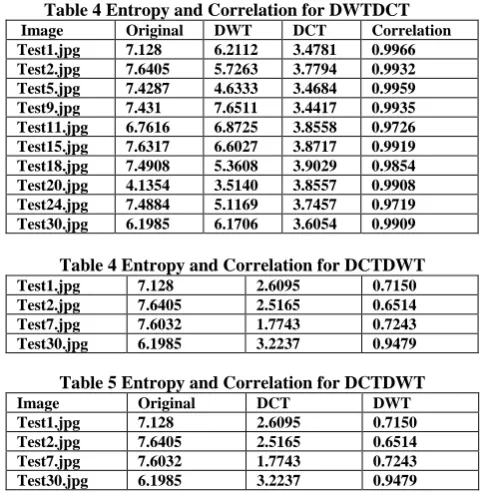
The neural network architecture consists of 4096 input neurons since the input image is of size 64 x64= 4096 pixels. Each neuron will represent one intensity value. There are eighty hidden layer neuron. Since we want the compression ratio for the range 10% to 90% there are 9 output neurons, each corresponding to the appropriate compression ratio. The architecture is as shown in figure 2.
In this case EBPTA (Error Back Propogation Training Algorithm) is used. Back propagation, or propagation of error, is a common method of teaching artificial neural networks how to perform a given task. It was first described by Arthur E. Bryson and Yu-Chi Ho in 1969, but it wasn't until 1986, through the work of David E. Rumelhart, Geoffrey E. Hinton and Ronald J. Williams, that it gained recognition, and it led to a “renaissance” in the field of artificial neural network research. It is a supervised learning method, and is an implementation of the Delta rule. It requires a teacher that knows, or can calculate, the desired output for any given input. It is most useful for feed-forward networks (networks that have no feedback, or simply, that have no connections that loop). The term is an abbreviation for "backwards propagation of errors". Back propagation requires that the activation function used by the artificial neurons (or "nodes") is differentiable. For better understanding, the back propagation learning algorithm can be divided into two phases: propagation and weight update.
Phase 1: Propagation
Each propagation involves the following steps:
1. Forward propagation of a training pattern's input through the neural network in order to generate the propagation's output activations.
2. Back propagation of the propagation's output activations through the neural network using the training pattern's target in order to generate the deltas of all output and hidden neurons.
Phase 2: Weight update For each weight-synapse:
1. Multiply its output delta and input activation to get the gradient of the weight.
2. Bring the weight in the opposite direction of the gradient by subtracting a ratio of it from the weight 3. This ratio influence he speed and quality of
learning; it is called the learning rate. The sign of the gradient of a weight indicates where the error is increasing, this is why the weight must be updated in the opposite direction.
Repeat the phase 1 and 2 until the performance of the network is good enough.
Back propagation networks are necessarily multilayer perceptron‟s (usually with one input, one hidden, and one output layer). In order for the hidden layer to serve any useful function, multilayer networks must have non-linear activation
functions for the multiple layers: a multilayer network using only linear activation functions is equivalent to some single layer, linear network. Non-linear activation functions that are commonly used include the logistic function, the softmax function, and the Gaussian functions.
We have used Back propagation algorithm for training neural network . The input set consists of 30 training pairs. The input layer consists of 4096 neurons. The output layer consists of 9 neurons. The hidden layer consists of 30 neurons. The network was trained and a sample during training is as shown below:
error=6.604521 no of epochs = 9999 error=6.604521 no of epochs = 10000 Elapsed time is 447.441998 seconds.
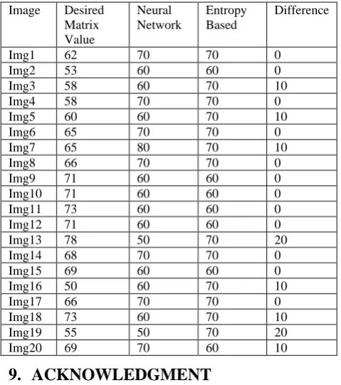
The above sample shows that the Neural network was trained using training set which consist of 30 images. It was then tested for set of set of testing images the result is depicted in Table 6. The desired matrix for NN was designed considering two different factors. The first was normal approach in which we design the desired matrix based on result obtained for set of training images especially compression ratio. But there is another factor term as entropy which is integral part of every image. The entropy of original image and compressed image on comparison yield either positive or negative result. If entropy of compressed image doesn‟t exceed original image entropy it‟s a positive result otherwise we term it as negative result. We trained the NN using both methodology and the testing result are shown in table 7. The comparison of both method is shown in table 8.
Table 4 Entropy and Correlation for DWTDCT
Image Original DWT DCT Correlation
[image:6.595.307.549.401.649.2]Test1.jpg 7.128 6.2112 3.4781 0.9966 Test2.jpg 7.6405 5.7263 3.7794 0.9932 Test5.jpg 7.4287 4.6333 3.4684 0.9959 Test9.jpg 7.431 7.6511 3.4417 0.9935 Test11.jpg 6.7616 6.8725 3.8558 0.9726 Test15.jpg 7.6317 6.6027 3.8717 0.9919 Test18.jpg 7.4908 5.3608 3.9029 0.9854 Test20.jpg 4.1354 3.5140 3.8557 0.9908 Test24.jpg 7.4884 5.1169 3.7457 0.9719 Test30.jpg 6.1985 6.1706 3.6054 0.9909
Table 4 Entropy and Correlation for DCTDWT
Test1.jpg 7.128 2.6095 0.7150
Test2.jpg 7.6405 2.5165 0.6514
Test7.jpg 7.6032 1.7743 0.7243
Test30.jpg 6.1985 3.2237 0.9479
Table 5 Entropy and Correlation for DCTDWT
Image Original DCT DWT
Test1.jpg 7.128 2.6095 0.7150
Test2.jpg 7.6405 2.5165 0.6514
Test7.jpg 7.6032 1.7743 0.7243
Test30.jpg 6.1985 3.2237 0.9479
7.
COMPARATIVE STUDY
Table 3 Result of DWT DCT Method with performance parameter
Image Name Original Image Compressed Image Parameters
Cameraman
Original Size=65KB Compressed Size=17KB MSE=177.07
RME=133.305 SNR=167.315 PSNR =13.050 Compression =75%
Test7.jpg
Original Size=13.3 KB Compressed Size=4.95 KB MSE=164.22
RME=128.149 SNR=168.388 PSNR =13.839
Test8.jpg
Original Size=8.13 KB Compressed Size=2.80 KB MSE=383.68
RME=195.877 SNR=165.158 PSNR =5.353 Compression =65.55%
Figure 2 Neural Network Architecture Table 7 Result of Testing Image
Image Entropy Correlation MSE RMSE SNR PSNR ORIG(Kb) COM(Kb) CR(%) MATRIX ENTROPY
Test1 7.1194 0.9813 1.486 121.91 166.128 14.836 14.8 6.38 56.89 6 7
Test2 7.7922 0.9896 2.477 157.411 165.637 9.726 10.6 4.18 60.56 6 8
Test3 7.276 0.992 9.441 97.166 166.247 19.375 11.5 5.39 53.13 5 7
Test4 6.9545 0.978 1.792 133.877 166.054 12.965 13.1 5.42 58.62 6 7
Test5 7.6928 0.977 1.6702 129.23 167.110 13.670 16.7 6.57 60.65 6 8
Test6 1.8818 0.993 5.314 230.527 165.692 2.069 7.01 3.37 51.92 5 2
Test7 7.090 0.989 1.083 104.099 166.712 17.996 10.9 5.06 53.57 5 7
Test8 7.5419 0.997 1.226 110.773 165.573 16.762 11.5 5.32 53.73 5 7
Test9 7.8861 0.988 1.525 123.51 166.580 14.575 15.4 6.21 59.67 6 8
Test10 6.7852 0.942 3.345 182.905 166.362 6.724 15.2 4.20 72.36 7 7
Test11 7.496 0.9611 1.960 140.011 168.560 12.069 19.2 6.21 67.65 7 7
Test12 7.4623 0.928 1.641 128.108 168.236 13.846 17.9 6.02 66.36 7 7
Test13 7.737 0.923 1.584 125.88 170.442 14.196 23.4 6.66 71.53 7 8
Test14 7.275 0.995 1.522 123.377 165.446 14.598 11.1 4.43 60.09 6 7
codeword are assigned to the corresponding symbols according to the probability of the symbols. The entropy encoders are used to compress the data by replacing symbol represented by the equal length codes with the code word‟s whose length is proportional to corresponding probability
8.
CONCLUSION
An enhanced BTC algorithm was proposed getting better image quality after compression. The method uses low pass filtering on the image first and then takes the DCT of given image, then implement the BTC. By applying DCT after low
pass filtering the number of pixels required for compression is reduced. A set of standard images were tested using different block size and image quality metrics were calculated. It was found that the reconstructed image has better quality compared to BTC. For 4x4 Block size 25% compression was achieved. Experimental results show that the difference between the pixel values of the original and the reconstructed image is considerably reduced. The test results also show the performance of the proposed method based on the parameters PSNR, MSE, Correlation and CR. The results show that the PSNR and MSE values are high when compared with BTC,
1
4096
2
1
2
80
1
9
OriginalImage
256 x 256 pixels
Reduced Image
64 x64 pixels
O
U
T
P
U
even when the compression ratio is same. It gives a better enhancement in the visual quality of the reconstructed images even at the edges. Further time taken by DCTBTC for encoding is less when compared with BTC as it involves simple calculations. The research works attempt to systematically design and then validate the compression technique. After the validation scope for optimization in that area of application will be taken in to consideration.
Regarding DWTDCT It can be concluded that result obtain indicate reduction in storage space requirement. This will directly help in reducing the transmission bandwidth requirement for various images. The second method provides better result compared to the first one. Moreover it is observed that time required to perform compression is reduce compared to traditional approach. In future these methods can be enhanced further by applying some other standard algorithm in mixed mode.
[image:8.595.49.288.336.608.2] [image:8.595.48.288.337.608.2]It can be concluded that result obtain indicate reduction in storage space requirement. This will directly help in reducing the transmission bandwidth requirement for various images. The design of NN helps in reducing the time requirement for calculating the compression ratio. The Neural network also helps in validating the result obtained before training by comparing them to result obtained after training
Table 8 Comparative study of NN methodologies
Image Desired Matrix Value
Neural Network
Entropy Based
Difference
Img1 62 70 70 0
Img2 53 60 60 0
Img3 58 60 70 10
Img4 58 70 70 0
Img5 60 60 70 10
Img6 65 70 70 0
Img7 65 80 70 10
Img8 66 70 70 0
Img9 71 60 60 0
Img10 71 60 60 0
Img11 73 60 60 0
Img12 71 60 60 0
Img13 78 50 70 20
Img14 68 70 70 0
Img15 69 60 60 0
Img16 50 60 70 10
Img17 66 70 70 0
Img18 73 60 70 10
Img19 55 50 70 20
Img20 69 70 60 10
9.
ACKNOWLEDGMENT
I would express my gratitude to my guide Dr Tanuja Sarode for her constant support and guidance. I would like to thank Prof Arun Kulkarni, Dean (AICTE Affairs) Dept of IT, Thadomal Shahani Engineering College for constant support, appreciation and advice in right direction. I am also thankful to Dr. G T Thampi, Principal TSEC, Dr. Subhash. K Shinde, Chairman Board of Studies Mumbai University for the valuable inputs and corrections suggested during course of research. I would also like to thank my wife Sonali and son Shlok for giving me space and time to carry out my work.
10.
REFERENCES
[1] Rafael C. Gonalez, Richard E.Woods “Digital Image Compression” 3rd
Edition, Prentice Hall.
[2] E. J.Delp, O R. Mitchelle “ Image Compression using Block truncation Coding” IEEE Transaction Communication 27(9) (1979) 1335-1342
[3] M. D. Lema, O.R . Mitchelle “Absolute Moment Block ytruncation Coding and its Application to Color Images” IEEE Transcaction Communication Vol COM-32, No.10, pp1148-1157 Oct 1984
[4] S.C .Cheng, W.S.Tsai “ Image Compression by moment-preserving edge detection” Pattern Recognition 27 (11) pp.1439- 1449
[5] U.Y Desai, M.M. Muzuki, B.K.P.Horn “Edge and mean based Compression” MIT Artifical Intelligence Laboratory AI Memo No.1584,November 1996.
[6] T.M.Ammarunnishad, V.K Govindan, T.M Abraham ” Improving BTC Image Compression using a Fuzzy Complement Edge operator”Signal Processing Letters, Vol 88. Issue 12 December 2008 pp. 2989-2997 [7] T.M.Ammarunnishad, V.K Govindan, T.M Abraham “ A
Fuzzy Complement edge operator “ IEEE proceeding of the Fourteen International Conference on Advance Computing and Communication Mangalore, Karnataka, India December 2006
[8] Aditya Kumar, Pradeep Singh “ Futuristic Algorithm for Gray Scale Image Based on Enhanced Block Truncation Coding” International Journal of Computer Information system Vol 2 No.5 pp 53-60 ,2011
[9] Jaymol Mathews, Madhu S Nair, Liza Jo ” Modified BTC Algorithm for Gray Scale Images Using max-min Quantizer” IEEE Transaction 2013 pp 377-382 [10]Manish Gupta, Dr. Anil Kumar Garg “Analysis of Image
Compression Algorithm Using DCT”, International Journal of Engineering Research and Applications ISSN:2248-9662, Vol 2 Issue 1 Jan-Feb2012 pp 515-521 [11]Mahinderpal Singh, Meenakshi Garg “Mixed DWT-DCT
Approached Based Image Compression Technique” International Journal of Engineering and Computer Science ISSN:2319-7242, Vol 3 Issue 11 November 2014 pp 9107-9111
[12]Bhavna Sagwan, Mukesh Sharma, Krishan Gupta “RGB based KMB Image Compression Technique” International Conference on Reliability, Optimization and Information Technology Feb 2014
[13] and Applications ISSN:2248-9662, Vol 2 Issue 1 Jan-Feb2012 pp 515-521
[14]Mahinderpal Singh, Meenakshi Garg “Mixed DWT-DCT Approached Based Image Compression Technique” International Journal of Engineering and Computer Science ISSN:2319-7242, Vol 3 Issue 11 November 2014 pp 9107-9111
[15]Bhavna Sagwan, Mukesh Sharma, Krishan Gupta “RGB based KMB Image Compression Technique” International Conference on Reliability, Optimization and Information Technology Feb 2014