Bias compensation recursive algorithm for dual rate rational models

A bias compensation on-line algorithm for dual-rate rational models

Jing Chen∗,a_{, Quanmin Zhu}b_{, Yanjun Liu}a

a_{School of Science, Jiangnan University, Wuxi 214122, PR China}

b_{Department of Engineering Design and Mathematics, University of the West of England, Bristol BS16 1QY, UK}

Abstract

In dual-rate rational systems, some output data are missing (unmeasurable) to make the traditional recursive least squares parameter estimation algorithms invalid. In order to overcome this difficulty, this paper develops a bias compensation recursive least squares algorithm for estimating the missing outputs and then the model parameters. The algorithm, based on auxiliary model and particle filter, has four integrated key functions, 1) to establish an auxiliary model to estimate unmeasurable outputs, 2) to compensate bias induced by correlated noise, 3) to add a filter to improve estimation accuracy of the unmeasurable outputs, 4) to obtain unbiased parameter estimation. Three examples are selected for simulation demonstrations to give further guarantees on the usefulness of the proposed algorithms. The comparative studies show that the bias compensation recursive least squares is more effective for such systems with dual-rate input and output data.

Key words: Parameter estimation, Recursive least squares, Auxiliary model, Particle filter, Rational model

1. Introduction

Nonlinear systems widely exist in engineering practice. When design robust controllers for nonlinear systems, researchers often assume that the parameters of the nonlinear systems are known in prior, such assumption may not be true in engineering practice. Thus parameter estimation plays an important role in system control. Recently, a number of identification algorithms have been developed. These algorithms can be roughly divided into two categories: One is the off-line algorithms, such as the least square (LS) algorithm [1, 2], the expectation-maximization algorithm and the variational Bayesian algorithm [3, 4]; The other is the on-line algorithms, such as the stochastic gradient algorithm [5, 6], the recursive least squares algorithm (RLS) and the maximum likelihood algorithm [7, 8]. Compared with the off-line algorithms, the on-line algorithms have less computational efforts and can update the parameters with new data, which makes the on-line algorithms more effective for implementation.

The rational model was first proposed in [9], where the rational model was considered as a special kind of nonlinear systems. Unlike the polynomial nonlinear systems which can be simplified as linear in the parameters and nonlinear in the regression terms, the rational model is defined as the ratio of two polynomial expressions [10]. The parameter identification for rational models is more challenging because a rational model is nonlinear in both the parameters and the regression terms. Since the rational model provides a very concise and parsimonious representation for complex nonlinear systems and has excellent extrapolation properties. The rational model identification is becoming a hot spot of present research [11, 12, 13, 14].

The off-line algorithms are the most widely used identification algorithms for rational models. For example, in [15], an error back propagation parameter estimation algorithm for a class of rational models was studied, and the rational model was depicted in a neural network structure. In [16], an implicit LS algorithm for rational models was proposed, where the algorithm is efficient in dealing with the parameter estimation problems associated with nonlinear in the parameters models. In [17], a globally consistent nonlinear LS estimator for identification of a nonlinear rational system was developed, in which the proposed off-line algorithm is the first globally convergent algorithm for the nonlinear rational systems. However, the off-line algorithms usually have heavy computational loads and cannot be used to update the parameters in real time when new data becomes

I_{This work is supported by the National Natural Science Foundation of China (No. 61403165), the Natural Science Foundation} of Jiangsu Province (No. BK20131109) and the Natural Science Foundation for Colleges and Universities in Jiangsu Province (No. 16KJB120006).

∗_{Corresponding author: School of Science, Jiangnan University, Wuxi 214122, PR China}

Email addresses: [email protected](Jing Chen),[email protected](Quanmin Zhu),yanjunliu [email protected]

available. In order to overcome these shortcomings of off-line algorithms, an enhanced linear Kalman filter algorithm for parameter estimation of nonlinear rational models was proposed in [18], in which the proposed algorithm is an on-line algorithm. Unfortunately, all the identification algorithms in the above work are limited to rational models whose input and output data are sampled at the same rate. When the rational model has dual-rate input and output data, these algorithms may be invalid. To the best of our knowledge, there is no work reported in the literature on identification of dual-rate rational models. Thus the focus of this paper is to develop a bias compensation on-line algorithm for rational models with dual-rate input and output data.

Dual-rate systems which the inputs and outputs are sampled at two different rates often exist in industrial [19]. For example, in polymer reactors, the manipulated variables can be adjusted at relatively fast rate, whereas the composition, density or molecular weight distribution measurements are typically obtained after several minutes of analysis [20]. The lifting and the polynomial transformation techniques are two main tools which are usually applied to deal with the dual-rate system identification [21, 22]. Both of these two methods first turn the original dual-rate system into a system containing all the input data and only the measured output data and then use all the measured data to estimate the unknown parameters. However, the complex structure of the rational model leads to the dual-rate system be impossible simplified as a systems containing all the measured data, thus these two methods cannot be utilized for rational model identification.

The auxiliary model is another effective method for systems with unmeasureable outputs [23]. Here, those unmeasureable outputs were replaced by the outputs of the auxiliary model, and then the unknown parame-ters were estimated based on the rich input data, the measured output data and the estimated output data. Compared with the lifting technique and the polynomial transformation technique, the auxiliary model method has no restriction to the polynomial of the output and can keep the number of the unknown parameters un-changed [24]. Thus the auxiliary model method is widely used for the dual-rate system identification [25, 26]. Unfortunately, the auxiliary model method only uses an auxiliary model to predict the missing outputs, while the measured outputs are not applied to improve the predicted outputs during the interval of the slow sampled rate, which makes the errors between the predicted outputs and the true missing outputs large. It is well known that the particle filter is an optimaltool for nonlinear state space model [27, 28]. Unlike the auxiliary model method, the particle filter uses the given data so far to improve the predicted states. Thus the particle filter method is more effective than the auxiliary model method [29, 30]. Nevertheless, the standard particle filter is only available for a state space model. In this paper, we will extend the particle filter to a non-state-space model.

This paper takes the above described literature into study, and proposes a bias compensation RLS based auxiliary model (BCRLS-AM) algorithm and a BCRLS based particle filter (BCRLS-PF) algorithm for a dual-rate rational model. In the BCRLS-AM algorithm, the unmeasureable outputs are estimated by the auxiliary model, while in the BCRLS-PF algorithm, the unmeasureable outputs are estimated by the particle filter and are improved by the measured outputs during each interval of the slow sampled rate. Thus the BCRLS-PF algorithm is more effective than the BCRLS-AM algorithm.

Briefly, the rest of this paper is organized as follows. Section 2 introduces the rational model and the RLS algorithm. Section 3 develops the BCRLS-AM algorithm. Section 4 studies the BCRLS-PF algorithm. Section 5 provides three examples. Finally, concluding remarks are given in Section 6.

2. The rational model and the RLS algorithm Consider the following rational model,

y(t) = a(t)

b(t) +e(t), (1)

where y(t) is the output, u(t) is the input, e(t) a stochastic white noise with zero mean and varianceσ, and a(t) andb(t) are expressed as

a(t) =φT_(t)θ

a,

b(t) =ψT

(t)θb.

The information vectorsφ(t) andψ(t) are the products of past inputs and past outputs, such asy(t−1)u(t−1), u(t−2) andu2(t−1)y(t−1), and the structures ofφ(t) andψ(t) are known in prior. θaandθbare the unknown

parameters to be estimated and can be expressed as

θb= [b1, b2,· · · , bm]T. (3)

Without loss of generality, assumeb1= 1, then the rational model can be simplified as

Y(t) =φT_(t)θ

a+y(t)[−ψT(t)θb+b1ψ1(t)] +b(t)e(t), (4)

whereY(t) =y(t)ψ1(t) andψ1(t) is the first element of the vector ψ(t). Rewriting Equation (4) as

Y(t) =ϕT

(t)θ+v(t), (5)

where

θ= [a1, a2,· · · , an, b2,· · ·, bm]T∈Rn+m−1,

ϕ(t) = [φ1(t), φ2(t),· · ·, φn(t),−y(t)ψ2(t),· · · ,−y(t)ψm(t)]T∈Rn+m−1,

v(t) =b(t)e(t).

For the dual-rate system, we assume that the output sampling period isqh(q>2 is an integer), while the input sampling period is h. Clearly, the output sampling period is an integer multiple of the input updating period. Then all the input data{u(t), t= 0,1,2,· · · }and some output data{y(tq), t= 1,2,· · · }are measureable, while the other outputs are unmeasureable.

Replacingtin (5) withtqgets

Y(tq) =ϕT_{(tq)θ+v(tq),}

ϕ(tq) = [φ1(tq), φ2(tq),· · ·, φn(tq),−y(tq)ψ2(tq),· · · ,−y(tq)ψm(tq)]T,

v(tq) =b(tq)e(tq).

Collecttqinput, output and noise data and define

Y(tq) := [Y(tq), Y(tq−q),· · · , Y(q)]T_,

Φ(tq) := [ϕ(tq),ϕ(tq−q),· · ·,ϕ(q)]T_,

V(tq) := [v(tq), v(tq−q),· · ·, v(q)]T_.

It follows that

Y(tq) =Φ(tq)θ+V(tq). (6)

Then the parametersθ can be estimated by the following LS algorithm,

ˆ

θ= [ΦT

(tq)Φ(tq)]−1ΦT

(tq)Y(tq). (7)

Compared with the LS algorithm, the RLS algorithm has less computational efforts, and can update the pa-rameters in real time when new data becomes available. Next, a RLS algorithm will be derived for the rational model,

ˆ

θ(tq) = [ΦT

(tq)Φ(tq)]−1ΦT

(tq)Y(tq)

=P(tq) [

Φ(tq−q)

ϕT_(tq)

]T[

Y(tq−q) Y(tq)

]

=P(tq)[(P−1(tq)−ϕT

(tq)ϕ(tq))ˆθ(tq−q) +ϕ(tq)Y(tq)]

= ˆθ(tq−q) +P(tq)ϕ(tq)[Y(tq)−ϕT

(tq)ˆθ(tq−q)]. (8)

Thus the RLS algorithm for estimating the parameter vector θ can be summarized as follows,

ˆ

θ(tq) = ˆθ(tq−q) +P(tq)ϕ(tq)[Y(tq)−ϕT

(tq)ˆθ(tq−q)],

P(tq) = [ΦT_(tq)Φ(tq)]−1_,

Φ(tq) = [ϕ(tq),ϕ(tq−q),· · · ,ϕ(q)]T_.

3. The BCRLS-AM algorithm

In order to make the RLS algorithm be an unbiased estimation algorithm, taking the conditional expectation on both sides of (7) gets

E (

ˆ

θ(tq) )

= E{[ΦT

(tq)Φ(tq)]−1ΦT

(tq)Y(tq)}

= E{[ΦT_(tq)Φ(tq)]−1_ΦT_(tq)(ΦT_{(tq)θ+V(tq))}}

=θ+P(tq)E{ΦT

(tq)V(tq)}, (9)

whereΦT_{(Lq)V(Lq) can be expressed as}

ΦT_{(tq)V(tq) = [ϕ(tq),ϕ(tq}−_q),· · · _,ϕ(q)]

     v(tq) v(tq−q)

.. . v(q)      =            

φ1(tq) · · · φ1(q)

φ2(tq) · · · φ2(q)

..

. . .. ...

φn(tq) · · · φn(q)

−y(tq)ψ2(tq) · · · −y(q)ψ2(q)

..

. . .. ...

−y(tq)ψm(tq) · · · −y(q)ψm(q)

                 b(tq)e(tq) b(tq−q)e(tq−q)

.. . b(q)e(q)     .

At time tq−q, all the input data and only the scarce output data{y(tq−q),· · ·, y(q)} are measureable. While the output datay(tq−1),· · ·, y(tq−q+ 1),· · ·, y(1) are unknown. In order to overcome this difficulty, an auxiliary model is introduced. The unknown output data are replaced with the outputs of the following auxiliary model,

ˆ

y(tq−k) = ˆa(tq−k) ˆ

b(tq−k)|θˆm(tq−q)

, k=q−1,· · ·,1,

where ˆθm(tq−q) is the unbiased parameter estimate vector attq−qand the subscript means the estimate of ˆ

a(tq₋k)

ˆ_b(tq−k) by using ˆθm(tq−q). Replacingyin ΦT(tq)V(tq) with ˆygets

ΦT_(tq)V(tq)≈_ΦˆT_{(tq) ˆV(tq)}

=             ˆ

φ1(tq) · · · φˆ1(q)

ˆ

φ2(tq) · · · φˆ2(q)

..

. . .. ...

ˆ

φn(tq) · · · φˆn(q)

−y(tq) ˆψ2(tq) · · · −y(q) ˆψ2(q)

..

. . .. ...

−y(tq) ˆψm(tq) · · · −y(q) ˆψm(q)

                 ˆ_b(tq)e(tq) ˆ

b(tq−q)e(tq−q) .. . ˆ b(q)e(q)     .

Unfortunately, ˆφi(xq), ˆψi(xq) and ˆb(xq) are time-varying, one cannot simplify t

∑

x=1

ˆ

φi(xq)ˆb(xq)e(xq) and

t

∑

x=1

ˆ

ψi(xq)ˆb(xq)e2(xq) as

E

[ _t

∑

x=1

ˆ

φi(xq)ˆb(xq)e(xq)

] = 0, E [ _t ∑ x=1 ˆ

ψj(xq)ˆb(xq)e2(xq)

] =σ2

t

∑

x=1

ˆ

Thus the parameter estimate vector ˆθm(tq−q) at timetq−qis applied to estimate the noisee(tq),

ˆ

e(tq) =y(tq)−ˆa(tq−k)

ˆ_b(tq−k)|θˆm(tq−q) ,

in which ˆe(tq) is the estimate ofe(tq). It follows that

ΦT_(tq)V(tq)≈_ΦˆT_{(tq) ˆV(tq)}

=             ˆ

φ1(tq) · · · φˆ1(q)

ˆ

φ2(tq) · · · φˆ2(q)

..

. . .. ...

ˆ

φn(tq) · · · φˆn(q)

−y(tq) ˆψ2(tq) · · · −y(q) ˆψ2(q)

..

. . .. ...

−y(tq) ˆψm(tq) · · · −y(q) ˆψm(q)

                

ˆ_b(tq)ˆe(tq) ˆ

b(tq−q)ˆe(tq−q) .. . ˆ b(q)ˆe(q)    

. (10)

Assume that ˆP(tq) is the estimate ofP(tq) and can be defined as

P(tq)≈Pˆ(tq) = [ ˆΦT(tq) ˆΦ(tq)]−1, (11)

ˆ

Φ(tq) = [ ˆϕ(tq),ϕˆ(tq−q),· · ·,ϕˆ(q)]T_{, (12)}

ˆ

ϕ(iq) = [ ˆφ1(iq),φˆ2(iq),· · ·,φˆn(iq),−y(iq) ˆψ2(iq),· · ·,−y(iq) ˆψm(iq)]T. (13)

Then the following theorem can be obtained.

Theorem 1: For the system in (5), when ˆθ(tq) is expressed by Equation (8), and ˆΦT(tq) ˆV(tq) and ˆP(tq) are expressed by Equations (10) and (11). Then the estimate ˆθm(tq) is an unbiased estimate of the parameter

vectorθ and can be expressed as

ˆ

θm(tq) = ˆθ(tq)−Pˆ(tq) ˆΦ

T

(tq) ˆV(tq). (14)

Proof: Taking the conditional expectation on both sides of Equation (14) gets

E [

ˆ

θm(tq)

] = E

[ ˆ

θ(tq)−Pˆ(tq) ˆΦT(tq) ˆV(tq) ] , which means E [ ˆ

θm(tq)

] = E [ ˆ θ(tq) ]

−_Pˆ_{(tq) ˆΦ}T

(tq) ˆV(tq). (15)

Substituting Equation (9) into Equation (15) gets

E [

ˆ

θm(tq)

]

=θ+P(tq)E{ΦT_(tq)V(tq)]−_Pˆ_{(tq) ˆΦ}T_{(tq) ˆV(tq).}

According to Equations (10) and (11), one can get

E [

ˆ

θm(tq)

]

=θ. (16)

Equation (16) declares that the estimate ˆθm(tq) is an unbiased estimate of parameter vectorθ.

Then the following BCRLS-AM algorithm for estimating the parameter vector is listed as follows:

ˆ

θm(tq) = ˆθ(tq)−Pˆ(tq) ˆΦ

T

(tq) ˆV(tq), (17)

ˆ

θ(tq) = ˆθ(tq−q) + ˆP(tq) ˆϕ(tq)[Y(tq)−ϕˆT(tq)ˆθ(tq−q)], (18) ˆ

θ(tq−k) = ˆθ(tq−q), k=q−1,· · ·,1, (19)

ˆ

ˆ

P(tq) = [ ˆΦT(tq) ˆΦ(tq)]−1, (21)

ˆ

Φ(tq) = [ ˆϕ(tq),ϕˆ(tq−q),· · ·,ϕˆ(q)]T_{, (22)}

ˆ

ϕ(iq) = [ ˆφ1(iq),φˆ2(iq),· · · ,φˆn(iq),−y(iq) ˆψ2(iq),· · · ,−y(iq) ˆψm(iq)]T, (23)

ˆ

e(tq) =y(tq)−ˆa(tq)

ˆ_b(tq)|θˆm(tq−q)

, (24)

ˆ

y(tq−k) = ˆa(tq−k) ˆ

b(tq−k)|θˆm(tq−q)

. (25)

The steps of computing the parameter estimation vector ˆθm(tq) by using the BCRLS-AM algorithm are

listed in the following.

1. Let ˆθ(0) =1/p0and ˆP(0) =p0Iwith1being a column vector whose entries are all unity,Ibe an identity

matrix of appropriate size andp0= 106.

2. Lett= 1,y(−j) = 0, u(−j) = 0, e(−j) = 0,j= 0,1,2,· · · , n−1, and give a small positive numberε. 3. Letk=q−1, and collect the input-output data{u(tq−q+ 1),· · ·, u(tq), y(tq)}.

4. Form ˆϕ(tq−k) by (23). 5. Form ˆΦ(tq−k) by (22).

6. Compute ˆy(tq−k) and ˆe(tq) by (25) and (24), respectively. Decrease k by 1, if k > 1, go to step 4; otherwise, go to next step.

7. Compute ˆP(tq) by (21).

8. Update the parameter estimation vector ˆθ(tq) by (18). 9. Compute ˆθm(tq) by (17).

10. Compare ˆθm(tq) and ˆθm(tq−q): if ∥θˆm(tq)−θˆm(tq−q)∥6ε, then terminate the procedure and obtain

the ˆθm(tq); otherwise, increaset by 1 and go to step 3.

Remark 1: According to Equations (17) and (18), we can conclude that the parameter estimates ˆθ(tq) by using the RLS-AM algorithm is biased, while the parameter estimates ˆθm(tq) by using the BCRLS-AM

algorithm is unbiased.

4. The BCRLS-PF algorithm

The particle filter is an optimal tool for nonlinear state space systems with unknown states [32]. In this section, we will extend the particle filter to dual-rate rational models.

4.1. The particle filter

In the particle filter, the missing outputs can be estimated by

ˆ

y(tq−k) =

N

∑

j=1

¯

ωjyˆj(tq−k),

in which ¯ωj is the weight associated with thejth particle and N

∑

j=1

¯

ωj = 1, ˆyj(tq−k) is the jth particle drawn

from the density function p(y(tq−k)|y(tq),· · ·, y(1), u(tq),· · ·, u(1),θ). In order to estimate ˆy(tq−k), one should get the weights ¯ωj and the particles ˆyj(tq−k),j= 1,· · · , N, respectively.

At timetq−q, the density function of the missing outputs can be expressed as

p(y(tq−k)|u(tq),· · ·, u(1), y(tq),· · ·, y(1),θˆm(tq−q))≈ N

∑

j=1

ωjδ(y(tq−k)−yˆj(tq−k)),

where δ(·) is the Dirac delta function andωj is the normalized weight associated with the jthparticle. The

samples{yˆj(tq−k)), j= 1,· · · , N}can be obtained from the following importance density q(·),

q(y(tq−k)|u(tq−k−1),· · · , u(1), y(tq),· · · , y(1),θˆm(tq−q)) =

From Equation (1), Equation (26) can be written as

q(y(tq−k)|u(tq−k),· · ·, u(1),y(tqˆ −k−1),· · · , y(tq−q),· · · ,y(1),ˆ θˆm(tq−q)) =

1 √

2πσexp 

₋(y(tq−k)−

ˆ a(tq₋k) ˆ

b(tq−k)|θˆm(tq−q) )2

2σ2



. (27)

Thus the new particles can be drew from Equation (27). According to [29], the weight of each new particle can be adjusted as follows,

ωj(tq) =p(y(tq)|yˆj(tq))ωj(tq−1), (28)

ωj(tq−k) =ωj(tq−k−1), k= 1,· · ·, q−1. (29)

However, the density function p(y(tq)|yˆj(tq)) cannot be obtained directly, which leads to the weight not be

updated. Define

||y(tq)−yˆj(tq)||:=γj(tq),

where || · ||is the 2 norm. Clearly, we can conclude that the smaller theγj(tq) is, the more important role of

thejthparticle at timetq in estimating the true outputy(tq) plays. Let

γ(tq) = max{γj(tq), j= 1,· · ·, N}+ 1,

then we can get

γj(tq)

γ(tq) <1, j= 1,· · ·, N.

Kernel density estimation is a non-parametric method to estimate the probability density function of a random variable. There are many kernel functions, the Epanechnikov kernel function is one of them and is optimal in a mean square error sense. In this paper, the Epanechnikov kernel function is introduced to obtain the density functionp(y(tq)|yˆj(tq)) [31],

p(y(tq)|yˆj(tq)) =

3 4

[

1−(γj(tq) γ(tq))

2

] .

By Normalizing the density function, the density functionp(y(tq)|yˆj(tq)) can be computed as

p(y(tq)|yˆj(tq)) =

γ2_(tq)−γ2 j(tq)

N γ2_(tq)− N ∑ j=1 γ2 j(tq) . (30)

Remark 2: If the measured datay(tq) is not applied to update the weight of each particle, then the density function is simplified asp(y(tq)|yˆj(tq)) = _N1 which is the same as that by using the auxiliary model method.

Theorem 2: Assume that the density functionp(y(tq)|yˆj(tq)) updated by the particle filter is expressed by

Equation (30), and the density function p(y(tq)|yˆj(tq)) updated by the auxiliary model method is 1/N, then

the following inequation holds

N

∑

j=1

γ2_(tq)−γ2 j(tq)

N γ2_(tq)− N

∑

j=1

γ2 j(tq)

(y(tq)−yˆj(tq))26 N

∑

j=1

1

N(y(tq)−yˆj(tq))

2_.

Proof: According to Equation (30), one can get

N

∑

j=1

γ2_(tq)−γ2 j(tq)

N γ2_(tq)− N

∑

j=1

γ2 j(tq)

(y(tq)−yˆj(tq))2− N

∑

j=1

1

N(y(tq)−yˆj(tq))

2

=

N

∑

j=1

−(N−1)γ2

j(tq) + N

∑

k=1,k̸=j

γ2 k(tq)

N(N γ2_(tq)− N

∑

k=1

γ2 k(tq))

SinceN(N γ2(tq)−

N

∑

k=1

γ_k2(tq)) is greater than zero, one only need to consider the following equation

N

∑

j=1



₋(N−1)γ_j2(tq) +

N

∑

k=1,k_̸=j

γ_k2(tq)  γ_j2(tq)

= [

(1−N)γ14(tq) +γ12(tq) N

∑

k=2

γk2(tq)

] +· · ·



(1₋N)γ₂4(tq) +γ₂2(tq)

N

∑

k=1,k̸=2

γ_k2(tq)  +· · ·



(1₋N)γj4(tq) +γ 2 j(tq)

N

∑

k=1,k̸=j

γk2(tq)

 +· · ·

[

(1−N)γ_N4(tq) +γ_N2(tq)

N_∑−1

k=1

γ_k2(tq) ]

=−

N

∑

k=2

(γ₁2(tq)−γ_k2(tq))2−

N

∑

k=3

(γ₂2(tq)−γ_k2(tq))2− · · ·

− N

∑

k=j+1

(γj2(tq)−γ 2 k(tq))

2_{− · · · −}

(γN2₋1(tq)−γ 2 N(tq))

2₆

0.

Clearly, the following inequation holds,

N

∑

j=1

γ2(tq)−γ_j2(tq)

N γ2_(tq)− N

∑

j=1

γ2_j(tq)

(y(tq)−yˆj(tq))26 N

∑

j=1

1

N(y(tq)−yˆj(tq))

2_.

Substituting Equation (30) into Equation (28) gets

ωj(tq) =

γ2_(tq)−γ2 j(tq)

N γ2_(tq)− N

∑

j=1

γ2 j(tq)

ωj(tq−1). (31)

Normalizing ωj(tq−k), k=q−1,· · · ,1,0 gets

¯

ωj(tq−k) =

ωj(tq−i) N

∑

j=1

ωj(tq−k)

. (32)

Then the estimate ofy(tq−k) can be computed as

ˆ

y(tq−k) =

N

∑

j=1

¯

ωj(tq−k)ˆyj(tq−k). (33)

The degeneracy phenomenon is an inevitable problem in the particle filter. In order to avoid this phe-nomenon, an effective sample sizeNef f is introduced [29],

Nef f =

1

N

∑

j=1

(¯ωj)2

. (34)

Given a thresholdNhold in prior,Nef f < Nhold means severe degeneracy. Thus we should use resampling. The

basic idea of resampling is to discard particles with small weights and concentrate on those particles with large weights, then assign the weight of each particles as ¯ωj= _N1.

1. Initialization: At timetq−q, drawN initial particles{yˆj(0)}Nj=1 from the prior densityp(y(0)|ˆθm(tq−q))

and set each particle’s weight to _N1. Collect the input data u(1),· · · , u(tq−q) and the output data y(q),· · ·, y(tq−q). Give a positive numberNhold.

2. Letk=q−1.

3. Collect{yˆj(tq−k)}Nj=1 from Equation (27).

4. Computeωj(tq−k) by Equation (28) or Equation (29).

5. Normalize ¯ωj(tq−k) from Equation (32).

6. Compute the missing output ˆy(tq−k) by Equation (33).

7. ComputeNef f by Equation (34) and compareNef f withNhold, ifNef f < Nhold, reset the weight of each

particle with ¯ωj(tq−k) = _N1 and go to next step; otherwise, go to next step.

8. Decrease kby 1, ifk>0 go back to step 3; otherwise terminate the procedure.

4.2. The identification algorithm

Since the unmeasureable outputs can be estimated by using the particle filter, then we can get the following BCRLS-PF algorithm:

ˆ

θm(tq) = ˆθ(tq)−Pˆ(tq) ˆΦ

T

(tq) ˆV(tq), (35)

ˆ

θ(tq) = ˆθ(tq−q) + ˆP(tq) ˆϕ(tq)[Y(tq)−ϕˆT(tq)ˆθ(tq−q)], (36) ˆ

θ(tq−k) = ˆθ(tq−q), k=q−1,· · ·,1, (37)

ˆ

θm(tq−k) = ˆθm(tq−q), (38)

ˆ

P(tq) = [ ˆΦT(tq) ˆΦ(tq)]−1, (39)

ˆ

Φ(tq) = [ ˆϕ(tq),ϕˆ(tq−q),· · ·,ϕˆ(q)]T_{, (40)}

ˆ

ϕ(iq) = [ ˆφ1(iq),φˆ2(iq),· · · ,φˆn(iq),−y(iq) ˆψ2(iq),· · · ,−y(iq) ˆψm(iq)]T, (41)

ˆ

e(tq−k) = ˆy(tq−k)−ˆa(tq−k) ˆ

b(tq−k)|θˆm(tq−q)

. (42)

The steps of computing the parameter estimate ˆθm(tq) by the BCRLS-PF algorithm are listed below.

1. Let ˆθ(0) =1/p0and ˆP(0) =p0Iwith1being a column vector whose entries are all unity,Ibe an identity

matrix of appropriate size andp0= 106.

2. Lett= 1,y(−j) = 0, u(−j) = 0, e(−j) = 0,j= 0,1,2,· · · , n−1, and give a small positive numberε. 3. Letk=q−1, and collect the input-output data{u(tq−q+ 1),· · ·, u(tq), y(tq)}.

4. Form ˆϕT(tq−k) by (41). 5. Form ˆΦ(tq−k) by (40).

6. Compute ˆy(tq−k) by the particle filter.

7. Compute ˆe(tq−k) by (42). Decreasek by 1, ifk>1, go to step 4; otherwise, go to next step. 8. Compute ˆP(tq) by (39).

9. Update the parameter estimation vector ˆθ(tq) by (36). 10. Compute ˆθm(tq) by (35).

11. Compare ˆθm(tq) and ˆθm(tq−q): if ∥θˆm(tq)−θˆm(tq−q)∥6ε, then terminate the procedure and obtain

the ˆθm(tq); otherwise, increaset by 1 and go to step 3.

Remark 3: It is observed from Theorem 2 that the output estimates by using the particle filter are more accurate than those by using the auxiliary model method, which means that the BCRLS-PF algorithm is more effective than the BCRLS-AM algorithm.

5. Examples

5.1. Example 1

Consider a dual-rate rational model proposed in [9] and assumeq= 2,

y(t) = 0.2y(t−1) + 0.1y(t−1)u(t−1) +u(t−1) 1 +y2_{(t−1) +y}2_(t−2) +

The rational model can be turned into the following model,

y(t) = 0.2y(t−1) + 0.1y(t−1)u(t−1) +u(t−1)−

y(t)y2(t−1)−y(t)y2(t−2) + 0.8e(t−1) +e(t),

the input{u(t)}is taken as a persistent excitation signal sequence with zero mean and unit variance, and{e(t)} is taken as a white noise sequence with zero mean and variance σ2 _{= 0.10}2_{. The parameter vectorθ and the}

information vectorϕ(t) can be expressed as

θ= [θT

a,θ

T

b]

T_{= [a}

1, a2, a3, b2, b3, b4]T= [0.2,0.1,1,1,1,0.8]T,

ϕ(t) = [φ1(t), φ2(t), φ3(t),−y(t)ψ2(t),−y(t)ψ3(t),−y(t)ψ4(t)]T

= [y(t−1), y(t−1)u(t−1), u(t−1),−y(t)y2(t−1),−y(t)y2(t−2), e(t−1)]T_.

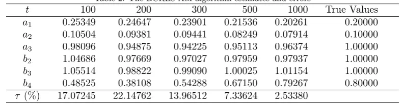
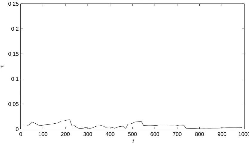
Apply the RLS-AM and the BCRLS-AM algorithms to estimate the parameters of the dual-rate rational model. The estimation errors τ:=∥θˆ−θ∥/∥θ∥ versust are shown in Figure 1. The parameter estimates and the estimation errors are shown in Tables 1 and 2, respectively. The estimated outputs, the true outputs and their errors are shown in Figure 2 (samples 800-900, BCRLS-AM).

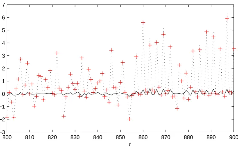
Next, we utilize the BCRLS-PF algorithm to estimate the parameters of the dual-rate rational model. The estimation errorsτ:=∥θˆ−θ∥/∥θ∥versustare shown in Figure 3. The parameter estimates and the estimation errors are shown in Table 3. The estimated outputs, the true outputs and their errors are shown in Figure 4 (samples 800-900).

Table 1: The RLS-AM algorithm estimates and errors

t 100 200 300 500 1000 True Values

a1 0.14913 0.15563 0.15636 0.13581 0.12754 0.20000

a2 0.09705 0.09182 0.09369 0.08587 0.08254 0.10000

a3 0.93340 0.90424 0.89770 0.90463 0.91546 1.00000

b2 0.91414 0.85764 0.85928 0.87741 0.88076 1.00000

b3 0.96020 0.90312 0.90746 0.91337 0.92589 1.00000

b4 0.41447 0.30767 0.37862 0.46169 0.53361 0.80000

τ (%) 21.12177 27.70588 24.32500 20.18904 16.73784

Table 2: The BCRLS-AM algorithm estimates and errors

t 100 200 300 500 1000 True Values

a1 0.25349 0.24647 0.23901 0.21536 0.20261 0.20000

a2 0.10504 0.09381 0.09441 0.08249 0.07914 0.10000

a3 0.98096 0.94875 0.94225 0.95113 0.96374 1.00000

b2 1.04686 0.97669 0.97027 0.97959 0.97937 1.00000

b3 1.05514 0.98822 0.99090 1.00025 1.01154 1.00000

b4 0.48525 0.38108 0.54288 0.67150 0.79267 0.80000

τ (%) 17.07245 22.14762 13.96512 7.33624 2.53380

Table 3: The BCRLS-PF algorithm estimates and errors

t 100 200 300 500 1000 True Values

a1 0.22417 0.23923 0.22300 0.22108 0.21968 0.20000

a2 0.09526 0.09860 0.09434 0.08776 0.08421 0.10000

a3 0.98862 0.99921 0.95220 0.97885 0.99325 1.00000

b2 1.00549 1.03026 0.97506 0.99805 0.98860 1.00000

b3 1.00977 1.03355 0.91320 0.96229 1.00540 1.00000

b4 0.24448 0.32093 0.35022 0.66103 0.80504 0.80000

τ (%) 28.95953 25.13350 24.04286 7.68273 1.53259

0 100 200 300 400 500 600 700 800 900 1000 0

0.1 0.2 0.3 0.4 0.5 0.6 0.7 0.8 0.9 1

RLS−AM

BCRLS−AM

t

τ

Figure 1: The parameter estimation errorsτ versust

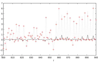
800 810 820 830 840 850 860 870 880 890 900

−3 −2 −1 0 1 2 3 4 5 6 7

t

Figure 2: Dotted line : the true outputs; +: the estimated outputs; black line: the output estimation errors (BCRLS-AM)

1. It is observed from Figures 1 and 3 that all the parameter estimation errors of these three algorithms decay whentis increased.

2. Figures 2 and 4 declare that the outputs estimated by using the BCRLS-PF algorithm are more accurate than those by using the BCRLS-AM algorithm.

0 100 200 300 400 500 600 700 800 900 1000 0

0.1 0.2 0.3 0.4 0.5 0.6 0.7 0.8 0.9 1

t

τ

Figure 3: The parameter estimation errorsτ versust(BCRLS-PF)

800 810 820 830 840 850 860 870 880 890 900

−3 −2 −1 0 1 2 3 4 5 6 7

t

Figure 4: Dotted line : the true outputs; +: the estimated outputs; black line: the output estimation errors (BCRLS-PF)

5.2. Example 2

In this example, a chemical model which is used to describe propylene catalytic oxidation is written as follows [16],

y(t) = k1Cp(t) 1 +k2

Cp(t)

C0.5

o (t)

+ v(t)

1 +k2 Cp(t)

C0.5

o (t) ,

where Co(t) and Cp(t) are the oxygen and propylene concentrations at time instantt respectively, and can be

andk2= 0.231.

In simulation, we manually impose q = 2. The inputs Co(t) and Cp(t) are taken as persistent excitation

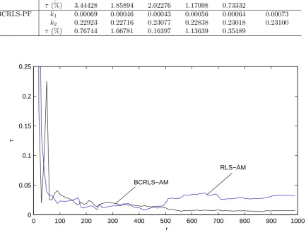
signal sequences with zero mean and unit variance, {v(t)} is taken as a white noise sequence with zero mean and varianceσ2= 0.102. Apply the RLS-AM, the BCRLS-AM and the BCRLS-PF algorithms to estimate the parameters of the dual-rate rational model. The estimation errors τ :=∥ˆθ−θ∥/∥θ∥ versust by using these three algorithms are shown in Figures 5 and 6. The parameter estimates and the estimation errors are shown in Table 4. From Figure 5, we can conclude that the BCRLS-AM algorithm is better than the RLS-AM algorithm, and from Table 4, we can get that the BCRLS-PF algorithm is the most effective algorithm among these three algorithms.

Table 4: The parameter estimates and errors

Algorithms t 100 200 300 500 1000 True Values

RLS-AM k1 0.00090 -0.00175 -0.00221 -0.00096 -0.00008 0.00073

k2 0.22563 0.23248 0.22909 0.22673 0.22332 0.23100

τ (%) 2.32408 1.25193 1.51540 1.98599 3.34285

BCRLS-AM k1 0.00091 -0.00178 -0.00230 -0.00099 -0.00008 0.00073

k2 0.23895 0.22752 0.23456 0.23309 0.23249 0.23100

τ (%) 3.44428 1.85894 2.02276 1.17098 0.73332

BCRLS-PF k1 0.00069 0.00046 0.00043 0.00056 0.00064 0.00073

k2 0.22923 0.22716 0.23077 0.22838 0.23018 0.23100

τ (%) 0.76744 1.66781 0.16397 1.13639 0.35489

0 100 200 300 400 500 600 700 800 900 1000

0 0.05 0.1 0.15 0.2 0.25

RLS−AM

BCRLS−AM

t

τ

Figure 5: The parameter estimation errorsτ versust

5.3. Example 3

The Michaelis-Menten model which is expressed for enzyme kinetics is considered as follows [12],

y(t) = β 1 + _u(t)α +

v(t) 1 + _u(t)α ,

0 100 200 300 400 500 600 700 800 900 1000 0

0.05 0.1 0.15 0.2 0.25

t

τ

Figure 6: The parameter estimation errorsτ versust(BCRLS-PF)

invalid. In this example, we assign the parameter estimates (the CLS-GN method) proposed in [17] to the unknown parameters: α= 0.0641 andβ = 212.6837, and assumeq= 2.

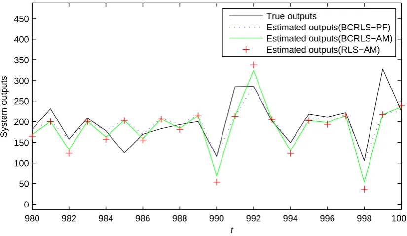
In simulation, the input{u(t)} is taken as a persistent excitation signal sequence with zero mean and unit variance. For a large β, in order to limit the noise to signal ratio to a reasonable level, we manually impose a white noise sequence{v(t)}with zero mean and varianceσ2= 52. Apply the RLS-AM, the BCRLS-AM and the BCRLS-PF algorithms to estimate the parameters of the dual-rate rational model. The comparisons of these three algorithms are shown in Table 5 (t=1000). The output estimates by using these three algorithms and the true output data are displayed in Figure 7 (samples 980-1000). From Table 5 and Figure 7, we can conclude that the BCRLS-PF algorithm is the most effective algorithm.

Table 5: The parameter estimates and errors Algorithms The parameter estimates τ (%)

RLS-AM α= 0.06386, β= 208.61513 1.91297 BCRLS-AM α= 0.06383, β= 209.01998 1.72261 BCRLS-PF α= 0.06381, β= 210.23803 1.14991

6. Conclusions

In research methodology, this study presents an example to integrate several across-boundary technical techniques to accommodate some challenging academic issues linked with wide range of applications. To the best of our knowledge, the BCRLS algorithm is the first on-line algorithm proposed for dual-rate rational models, and it is believed that this study will bring forward a new direction in using on-line algorithm to identify rational models with time-delay, random missing observations and colored noise.

In technique development/novelty, a BCRLS-AM algorithm is proposed for dual-rate rational models in this paper, in which the unmeasurable outputs are estimated by an auxiliary model. Based on the rich input data, the measureable output data and the estimated output data, the unknown parameters can be estimated by the BCRLS-AM algorithm. In order to increase the estimation accuracy of the BCRLS-AM algorithm, a BCRLS-PF algorithm is developed. Furthermore, these two algorithms can also be extended to rational models with random missing outputs.

980 982 984 986 988 990 992 994 996 998 1000 0

50 100 150 200 250 300 350 400 450

t

System outputs

True outputs

Estimated outputs(BCRLS−PF) Estimated outputs(BCRLS−AM) Estimated outputs(RLS−AM)

Figure 7: The true outputs and the estimated outputs

In further research, there are still some interesting topics not discussed in this paper. For example, if the denominator and numerator polynomial terms contain noise terms, how to eliminate the bias in the RLS algorithm. Another topic is how to prove the convergence properties of the BCRLS-PF algorithm. These topics will remain as the challenging issues in the future.

References

[1] H. Sarmadi, A. Karamodin, A. Entezami, A new iterative model updating technique based on least squares minimal residual method using measured modal data, Applied Mathematical Modelling 40 (23-24) (2016) 10323-10341.

[2] F. Ding, F.F. Wang, L. Xu, et al., Decomposition based least squares iterative identification algorithm for mul-tivariate pseudo-linear ARMA systems using the data filtering, Journal of the Franklin Institute 354 (3) (2017) 1321-1339.

[3] F.Y. Chen, F. Ding, The filtering based maximum likelihood recursive least squares estimation for multiple-input single-output systems, Applied Mathematical Modelling 40 (3) (2016) 2106-2118.

[4] Y.J. Lu, B. Huang, S. Khatibisepehr, A variational Bayesian approach to robust identification of switched ARX models, IEEE Transactions on Cybernetics 46 (12) (2016) 3195-3208.

[5] D.Q. Wang, L. Mao, F. Ding, Recasted models based hierarchical extended stochastic gradient method for MIMO nonlinear systems, IET Control Theory and Applications 11 (4) (2017) 476-485.

[6] L. Xu, F. Ding, The parameter estimation algorithms for dynamical response signals based on the multi-innovation theory and the hierarchical principle, IET Signal Processing 11 (2) (2017) 228-237.

[7] D.Q. Wang, Y.P. Gao, Recursive maximum likelihood identification method for a multivariable controlled autore-gressive moving average system, IMA Journal of Mathematical Control and Information 33 (4) (2016) 1015-1031.

[8] D.Q. Wang, Z. Zhang, J.Y. Yuan, Maximum likelihood estimation method for dual-rate Hammerstein systems, International Journal of Control, Automation and Systems 15 (2) (2017) 698-705.

[10] Q.M. Zhu, Z. Ma, K. Warwick, Neural network enhanced generalised minimum variance self-tuning controller for nonlinear discrete time systems, IEE Proceedings Control Theory and Applications 146 (4) (1999) 319-326.

[11] E. Klipp, R. Herwig, A. Kowald, Systems biology in practice: concepts, implementation and application, Weinheim, Germany: Wiley-VCH, (2005).

[12] D.M. Bates, D.G. Watts, Nonlinear regression analysis and its applications, Hoboken, NJ: John Wiley & Sons, (2007).

[13] S.A. Billings, K.Z. Mao, Structure detection for nonlinear rational models using genetic algorithms, International Journal of Systems Science 29 (3) (1998) 223-231.

[14] Q.M. Zhu, Y.J. Wang, D.Y. Zhao, et al., Review of rational (total) nonlinear dynamic system modelling, identifica-tion and control, Internaidentifica-tional Journal of Systems Science 46 (12) (2015) 2122-2133.

[15] Q.M. Zhu, A back propagation algorithm to estimate the parameters of nonlinear dynamic rational models, Applied Mathematical Modelling 27 (3) (2003) 169-187.

[16] Q.M. Zhu, An implicit least squares algorithm for nonlinear rational model parameter estimation, Applied Mathe-matical Modelling 29 (7) (2005) 673-689.

[17] B.Q. Mu, E.W. Bai, W.X. Zheng, et al., A globally consistent nonlinear least squares estimator for identification of nonlinear rational systems, Automatica 77 (2017) 322-335.

[18] Q.M. Zhu, D.L. Yu, D.Y. Zhao, An enhanced linear Kalman filter (EnLKF) algorithm for parameter estimation of nonlinear rational models, International Journal of Systems Science 48 (3) (2017) 451-461.

[19] D.Q. Wang, H.B. Liu, F. Ding, Highly efficient identification methods for dual-rate Hammerstein systems, IEEE Transactions on Control Systems Technology 23 (5) (2015) 1952-1960.

[20] Y.J. Liu, F. Ding, Y. Shi, An efficient hierarchical identification method for general dual-rate sampled-data systems, Automatica 50 (3) (2014) 962-970.

[21] D. Li, S. Shah, T. Chen, Analysis of dual-rate inferential control systems, Automatica 38 (6) (2002) 1053-1059.

[22] J. Ding, F. Ding, X.P. Liu, et al., Hierarchical least squares identification for linear SISO systems with dual-rate sampled-data, IEEE Transactions on Automatic Control 56 (11) (2011) 2677-2683.

[23] F. Ding, F.F. Wang, L. Xu, et al., Parameter estimation for pseudo-linear systems using the auxiliary model and the decomposition technique, IET Control Theory and Applications 11 (3) (2017) 390-400.

[24] J. Chen, Several gradient parameter estimation algorithms for dual-rate sampled systems, Journal of the Franklin Institute 351 (1) (2014) 543-554.

[25] J. Chen, R. Ding, An auxiliary-model-based stochastic gradient algorithm for dual-rate sampled-data Box-Jenkins systems, Circuits, Systems and Signal Processing 32 (5) (2013) 2475-2485.

[26] F. Ding, X.M. Liu, Y. Gu, An auxiliary model based least squares algorithm for a dual-rate state space system with time-delay using the data filtering, Journal of the Franklin Institute 353 (2) (2016) 398-408.

[27] T. Yang, R.S. Laugesen, P.G. Mehta, et al., Multivariable feedback particle filter, Automatica 71 (2016) 10-23.

[28] E. Ozkan, V. Smidl, S. Saha, et al., Marginalized adaptive particle filtering for nonlinear models with unknown time-varying noise parameters, Automatica 49 (6) (2013) 1566-1575.

[29] J. Deng, B. Huang, Identification of nonlinear parameter varying systems with missing output data, AIChE Journal 58 (2012) 3454-3467.

[30] D. Simon, Optimal State Estimation: Kalman, H∞, and Nonlinear Approaches, John Wiley & Sons, Inc., New Jersey, (2006).

[31] L. Qi, R.J. Racine, Nonparametric Econometrics: Theory and Practice, Princeton University Press, (2007).