Application of Statistical Methods to Assess Carbon Monoxide Pollution Variations within an Urban Area

Application of Statistical Methods to Assess Carbon

Monoxide Pollution Variations within an Urban Area

Carmen Capilla

Department of Applied Statistics and Operations Research and Quality, Universidad Politécnica de Valencia, Valencia, Spain Email: [email protected]

Received June 22, 2012; revised July 28, 2012; accepted August 24, 2012

ABSTRACT

In recent years there have been considerable new legislation and efforts by vehicle manufactures aimed at reducing pollutant emission to improve air quality in urban areas. Carbon monoxide is a major pollutant in urban areas, and in this study we analyze monthly carbon monoxide (CO) data from Valencia City, a representative Mediterranean city in terms of its structure and climatology. Temporal and spatial trends in pollution were recorded from a monitoring net- work that consisted of five monitoring sites. A multiple linear model, incorporating meteorological parameters, annual cycles, and random error due to serial correlation, was used to estimate the temporal changes in pollution. An analysis performed on the meteorologically adjusted data reveals a significant decreasing trend in CO concentrations and an an- nual seasonal cycle. The model parameters are estimated by applying the least-squares method. The standard error of the parameters is determined while taking into account the serial correlation in the residuals.The decreasing trend im- plies to a certain extent an improvement in the air quality of the study area. The seasonal cycle shows variations that are mainly associated with traffic and meteorological patterns. Analysis of the stochastic spatial component shows that most of the intersite covariances can be analyzed using an exponential variogram model.

Keywords: Carbon Monoxide; Monitoring Network; Statistical Model; Urban Air Pollution

1. Introduction

Urban air quality has become an important issue.During the last few years there has been considerable new legis- lation and efforts by vehicle manufactures aimed at re- ducing pollutant emissions and improving air quality in urban areas. Air quality monitoring commonly provides online information of urban emissions. Analysis of this information enables us to determine whether the envi- ronment is improving or deteriorating [1]. Such analysis can be useful in avoiding, preventing, and reducing the harmful effects of pollution on human health and the environment as a whole.

An important source of air pollutants within cities is traffic. A high density of emissions affects air quality [2]. Shahgedanova et al. [3] presented a study of air pollution within a city, considering carbon monoxide (CO) as an air quality indicator. They observed a strong increase in CO over time as well as a seasonal cycle related to sea- sonal variations in patterns of vehicular emissions. The major source of CO in such settings is internal combus- tion engines. Fernandez et al. [4] analysed long-term variations in pollution trends in Madrid, Spain, and found that CO had the highest concentrations of any pollutant in the urban air mass. The concentration of CO shows

temporal and spatial variability reflecting local traffic trends.

Other assessments of air quality in urban areas are pro- vided by [5] and [6]. Kimmel and Kaasik [5] analysed a database of air pollution sources (NOx and CO from in-

dustry, traffic, and domestic heating sources). They checked the database values against measured concentra- tions and predicted concentrations patterns associated with various traffic scenarios. Chaloulakou et al. [6] pre- sented a statistical analysis of PM10, PM2.5, and black

smoke in Athens over a 2-year period. Other work on pedestrian exposure to air pollutants such as CO within an urban area can be found in [7], who concluded that relatively high exposure levels of CO are strongly traf- fic-related and vary significantly with traffic conditions and street configuration. An analysis of the relationship between pollutants, including CO, and varying traffic density can be found in [8].

work was installed that year. The ground-level network provides online information on several pollutants drawn from five sampling sites. The network is managed by the Laboratory of Chemistry and Environment of the Valen- cia Town Hall. The outline of the remainder of the paper is as follows. Section 2 presents the dataset and the me-thodology employed in the present analysis. Section 3 contains the results and a discussion of the model estima- tion. Finally, concluding remarks are presented in Sec- tion 4.

2. Materials and Methods

2.1. Monitoring Network and Dataset

Figure 1 shows the location of the air-pollution moni-

toring network, which consists of five regularly operating sites. Table 1 provides station names, geographical co- ordinates, brief description of locations and number of samples. The altitudes of all stations are around 11 m above sea level. The sampling network enables real-time recording and analysis of the pollution levels of several air quality indicators.

Samples have been collected continuously since 1994. This paper considers analyses of monthly CO data, and is part of a larger project with the aim of assessing the air quality in Valencia City. In comparison with other Span- ish cities [4], air quality in Valencia remains been poorly researched.

In this study, CO is measured in mg/m3 _{using non-}

dispersive infrared absorption technology. Figure 2 shows monthly aggregated CO time series data recorded at the five sampling sites from January 1994 to Decem- ber 2004. In this paper, temporal variations of CO are studied at this monthly scale. Analyses and graphs have been obtained using the language and environment “R” [9].

1 ARAGON 2 GRAN VÍA 3 LINARES 4NUEVO CENTRO

5 PISTA DE SILLA

[image:2.595.307.538.104.548.2]

Figure 1. Map of Valencia City and locations of the auto-matic network sites.

Table 1. Locations and general characteristics of sampling stations in Valencia City.

Station Coordinates Station environment Number of _samples 0˚21'17''W,

39˚28'37''N

Roadside site 200 m from a motorway access road

ARAGON 113

G.VIA 0₃₉˚23'21''W,

˚28'05''N

Street intersection in downtown Valencia with high traffic density 98

LINARES 0₃₉˚23'16''W,

˚28'52''N

Street intersection in downtown Valencia with high traffic density

132

N.CENTRO 0₃₉˚22'32''W,

˚27'33''N

Roadside site in central Valencia close to a shopping center and a motorway access road

132

P.SILLA 0₃₉˚22'52''W,

˚28'05''N

Roadside site several meters from a motorway 132

0 20 40 60 80 100 120 140

024

6

Number of observation

M

ont

hl

y

av

er

age

C

O

c

onc

ent

rat

ion

[image:2.595.308.537.114.536.2]

ARAGON G.VIA LINARES N.CENTRO P.SILLA

Figure 2. Time series plot of monthly averaged carbon mo-noxide concentrations in mg/m3 recorded at the five sam-pling sites from January 1994 until December 2004.

[image:2.595.112.233.525.709.2]

The highest CO concentrations are observed at Station 1 (ARAGON), located just several meters from a mo- torway, while the lowest concentrations are recorded at Station 5 (P.SILLA). Similar long-term patterns are re- corded at the five stations. An exponential decreasing trend in the five sets of time series data is apparent in

Figure 2. Fluctuations around the trend component ex-

ponents of the series data combine multiplicatively. An analysis of deviation from normality shows that a loga- rithmic transformation is appropriate for a normal distri- bution in the data.

As an example, Figure 3 shows a histogram of data from Station 1 (ARAGON), in which a right-skewed unimodal frequency distribution is apparent. Right- skewness of the frequency distribution of air pollutant concentrations has also been observed in previous studies [10,11]. The natural log transformation also makes the series model additive, which would then have a linear trend component.

2.2. Analysis of Temporal Components

The graphical analysis in Figure 2 indicates that the log CO concentration observed at a specific location s and month t can be represented by temporal t and stochastic

components et(s):

 

 

log COt s te st . (1)

The temporal term t models the trend component, the

effect of meteorological conditions, and the annual cycle:

6

1

2π 2π

cos sin

12 12

t t t

i i

i

t T vS W

it it

    

 



    



 _ 





t

  

(2)

where t is time in months, Tt is monthly temperature, Stis

total sunshine hours, and Wt the average wind speed.

These are meteorological variables that are known to be significant predictors of other pollutants such as ozone

Histogram of CO

CO concentration

1 2 3 4 5 6

F

requ

enc

y

0

5

10

1

5

2

[image:3.595.61.289.485.700.2]

0

Figure 3. Histogram of monthly averages of carbon mon-oxide (mg/m3) recorded at Station 1 (ARAGON).

[12]. The seasonal cycle is modelled using trigonometric regressors. For the purpose of trend estimation, regres- sion modelling has been widely used to model pollutants as a function of meteorological parameters; this approach has demonstrated capability of detecting trends that are disguised by meteorological variations. Vingarzan and Taylor [12] and Rao and Zurbenko [13] provide applica- tions of regression models to study trends in ozone con- centrations. CO is a pollutant that is known to be in- volved, although in a minor way, in chemical reactions leading to the production of photochemical smog. The degree of activation of these photochemical reactions depends on meteorological effects [2] that are taken into account in (2). The term  therefore represents the slope of the trend after adjustment for meteorological factors and for cycles of various time periods. , , θ, ν, ω, i,

and i are the parameters to be estimated.

One of the most commonly used methods for fitting a linear model such as (2) is the ordinary least squares (OLS) technique. When the OLS estimation method is applied, the inference step assumes that the residuals are independent random errors from a normal distribution [14]. The residuals et follow the normal distribution after

applying the log transformation to the original right- skewed observations. Analysis of residual autocorrela- tion after OLS fitting of (2) indicates that they are de- pendent and follow a first-order stationary autoregressive model:

1 t t

e e at, (3)

where at is independent normal value with mean 0 and

variance 2 a

 . The main effect of the autocorrelation of the residuals on the OLS estimation is an inaccurate es- timation of the variance of the parameters. This has an impact on the tests of the statistical significance of the model parameters. The OLS estimates of the model coef- ficients are still unbiased, however, the test of signifi- cance is meaningless [15]. Taking into account the re- siduals autoregressive model, the covariance matrix of the parameters vector b can be derived using the expres- sion:

 

2



 

 



1

Cov a X  T X 

 

b , (4)

where X

 

 is the matrix with the Xi regressors:

 

2,1 1,1 2, 1,

,1 1,1 , 1,

1 .... .

. . . . . .

. . . . . .

1 . . . . .

I I

n n n I n I

X X X X

X

X X X X

  



  _  _

    

 

 

  

 

  

 

 

(5)

2.3. Spatial Analysis

appropriately de-trended data. Geostatistical techniques can be used to analyse this component [16,17]. An im- portant parameter for describing the spatial covariation of the random process is the variogram. For a de- tailed explanation of the variogram estimation and prop- erties see Cressie [16]. The variogram estimate is ob- tained via the expression:

 

t

e s

2

 

h Var_e_t

 

s_i e s_t

 

_{j } (6) This parameter is expressed as a function of intersite distances i j . Fitting a variogram function to a

plot of (6) values enables an estimate of

 for any two monitored or potentially

monitored sites si and sj. The estimated covariance func-

on can subsequently be used in kriging-based techniques

to compute the stochastic omponent and the

standard error of these estimates.

h s s



 

 

are st i e st j

 

t

e s

3. Results and Discussion

Trend estimation using (2) and the method detailed above provides the results [–0.016, –0.009] mg/m3 _{in the}

[image:4.595.311.537.81.330.2] [image:4.595.312.537.373.617.2]

log scale (95% confidence interval). Transforming back to the original scale, this indicates a decrease in CO con- centrations of between 10.5% and 17.6% over a period of 12 months. Statistically significant meteorological pre- dictors are total sunshine hours and wind speed.

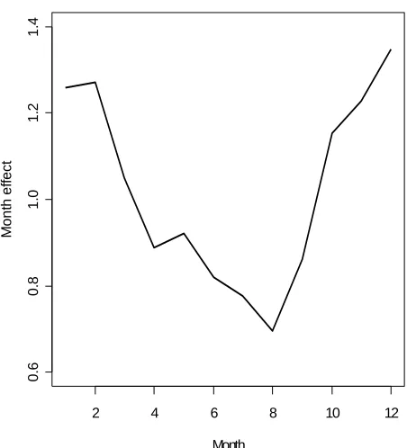
Figure 4 provides a plot of the estimated annual cycle

using the linear model approach. The seasonal compo- nent is clearly associated with annual traffic patterns and climatological variations. As Shahgedanova et al. [3] indicated, CO is a relatively inert pollutant. Therefore, its seasonal cycle depends on the emission rate and mete- orological variations. Traffic patterns in Valencia City show clear seasonal variations, with increasing activity during the coldest months from September to February. CO emissions are higher during times of lower tempera- tures. They also increase with reduced traffic speed.

Reduced traffic speed occurs in Valencia during winter months when central city locations have a greater density of traffic. All these factors affect the seasonal variability shown in Figure 4, resulting in minimum CO concentra- tions during the summer months and higher values dur- ing autumn and winter. The coefficient of determination of the multiple linear model with the trend, meteorologi- cal covariates, seasonal component, and autoregressive residuals results in 93.01%, which explains a high per- centage of the observed variability in the data.

Figure 5 displays the empirical estimation (6)

against geographical distance (m) between sites over the entire network.

 

h



The last value plotted in Figure 5 with a different symbol corresponds to the 

 

h value between Stations 1 and 3, and is the only one that does not show an increas-

2 4 6 8 10 12

0.

6

0.

8

1

.0

1.

2

1.

4

Month

M

o

nt

h e

ff

e

c

t

Figure 4. Annual cycle estimation using a statistical linear model.

0 500 1000 1500 2000 2500 3000

0.

00

0.

05

0.

10

0.

15

0.

20

0.

25

Distance (m)

G

a

mma

Figure 5. Empirical semivariogram versus geographical distance (m) with fitted exponential function.

ing trend of 

 

h with distance. The value be- een Stations 1 and 3 reflects the similarity in values ob-served at these two stations despite their geographical separation. Figure 5 also represents the variogram fit. The exponenttial semivariogram (7) was chosen after visual inspection of the graph:

 

h

 

1

_

2

_

3

0

exp 0

2

h h

h h

  

 

 



  _

  . (7)

The parameters are the asymptotic range 3, sill 2,

and nugget effect 1, which were computed using the

weighted least squares approach [18]. The sum of the sill and nugget equals 0.14, which is similar to the variance of et (0.137). This finding is consistent with the theory

behind semivariograms.

The spatial variability analysis can be used to imple- ment a spatial interpolation technique that predicts the stochastic component at a location s, . Optimal prediction of this component can be computed from available observations using kriging estimation [16]. The estimated spatial component is combined with the tem- ral component according to (1) to predict CO concentra- ons at time t and location s.

 

t

e s

This approach has been used to estimate the field of CO concentrations over the study area for January 2005; however, for Stations 1 (ARAGON) and 2 (G.VIA), there are no available measurements for this period. The mean value of the predicted field (0.56 mg/m3_{) provides}

[image:5.595.321.519.78.318.2]

an estimate of the CO concentration over the entire study area.

Figure 6 shows the prediction surface. Figure 7 repre-

sents the contour plot with the standard error of the pre- diction (the red numbers indicate the station locations). The estimation results and their accuracy are satisfactory. It captures the major features observedin the empirical CO concentrations over the entire monitored area.

Finally, complete content and organizational editing before formatting. Please take note of the following items when proofreading spelling and grammar.

4. Concluding Remarks

The temporal and spatial variability of monthly averaged carbon monoxide concentrations has been modeled using

Longitu_{de U.T} .M. Pro

jection _(m)

Latit ude

U.T .M. P

roje ctio

n (m )

K rig ing

p red ic tio_n

o f C O c_on

c_en

[image:5.595.63.286.548.715.2]

trat io n

Figure 6. Prediction of carbon monoxide for January 2005.

725000 725500 726000 726500 727000 727500

4371000

4372000

437300

0

Longitud U.T.M. Projection (m)

L

at

it

ude U

.T

.M

. P

roj

ec

ti

on (

m

) 1

2 3

4

5

Figure 7. Estándar error of the prediction.

data gathered over an 11-year period at Valencia, Spain. The monitored sites have different environments but are all located in regions of high traffic density.

Preliminary graphical analysis indicates that monthly observations can be modeled with a temporal component and a stochastic spatial component. The temporal com- ponent includes an exponential trend and an annual sea- sonal cycle. After applying a natural log transformation to the data, a linear model is estimated using ordinary least squares. Temporal correlation of the residuals of the linear model is taken into account when computing the standard error of the model parameters.

The results indicate a significant downward trend in CO concentrations over the study period, with the trend following an exponential pattern. In terms of CO pollu- tion, air quality has improved since 1994. The seasonal cycle is associated with traffic and climate patterns in Valencia. Autumn and winter months, which are charac- terized by lower temperatures and higher traffic volumes, record the highest carbon monoxide concentrations.

and spatial components can be used to predict CO con- centrations. The accuracy of the prediction is estimated using the variance of the temporal and spatial interpola- tion. This technique captures the main features of the empirical field and is satisfactory in terms of the predic- tion error.

REFERENCES

[1] E. P. Smith, S. Rheem and G. I. Holtzman, “Multivariate Assessment of Trend in Environmental Variables,” In: G. P. Patil and C. R. Rao, Eds., Multivariate Environmental Statistics, Elsevier Science Publishers, North-Holland, 1993, pp. 489-507.

[2] P. Brimblecombe, “Air Composition and Chemistry,” 2nd Edition, Cambridge University Press, Cambridge, 1995. [3] M. Shahgedanova, T. P. Burt and T. D. Davies, “Carbon

Monoxide and Nitrogen Oxides Pollution in Moscow,” Water Air and Soil Pollution, Vol. 112, No. 1-2, 1999, pp. 107-131. doi:10.1023/A:1005043916123

[4] M. T. Fernandez-Jiménez, A. Climent-Font and J. L. Sánchez-Antón, “Long Term Atmospheric Pollution Stu- dy at Madrid City (Spain),” Water, Air and Soil Pollution, Vol. 142, No. 1-4, 2003, pp. 243-260.

doi:10.1023/A:1022011909134

[5] V. Kimmel and M. Kaasik, “Assessment of Urban Air Quality in South Estonia by Simple Measures,” Environ-mental Modelling and Assessment, Vol. 8, No. 1, 2003, pp. 47-53. doi:10.1023/A:1022449831456

[6] A. Chaloulakou, P. Kassomenos, G. Grivas and N. Spy-rellis, “Particulate Matter and Black Smoke Levels in Central Athens, Greece,” Environment International, Vol. 31, No. 5, 2005, pp. 651-659.

doi:10.1016/j.envint.2004.11.001

[7] L. Zhao, X. Wang, Q. He, H. Wang, G. Sheng, L. Y. Chan, J. Fu, and D. R. Blake, “Exposure to Hazardous Volatile Organic Compounds, PM10 and CO While Walk-

ing Along the Streets in Urban Guangzou, China,” At- mospheric Environment, Vol. 38, No. 25, 2004, pp. 6177-6184. doi:10.1016/j.atmosenv.2004.07.025

[8] J. Beauchamp, A. Wisthaler, W. Grabmer, C. Neuner, A. Weber and A. Hansel, “Short Term Measurements of CO, NO, NO2, Organic Compounds and PM10 at a Motorway

Location in an Austrian Valley,” Atmospheric Environ-ment, Vol. 38, No. 16, 2004, pp. 2511-2522.

doi:10.1016/j.atmosenv.2004.01.032

[9] Development Core Team, “A Language and Environment for Statistical Computing,” Foundation for Statistical Computing, Vienna, 2011. http://www.R-project.org [10] W. R. Ott, “A Physical Explanation of the Lognormality

of Pollutant Concentrations,” Journal of the Air and Waste Management Association, Vol. 40, No. 10, 1990, pp. 1378-1383. doi:10.1080/10473289.1990.10466789 [11] C. K. Lee, “Multifractal Characteristics in Air Pollutant

Concentration Time Series,” Water, Air and Soil Pollu-tion, Vol. 135, No. 1-4, 2002, pp. 389-409.

doi:10.1023/A:1014768632318

[12] R. Virgarzan, and B. Taylor, “Trend Analysis of Ground Level Ozone in the Greater Vancouver/Fraser Valley Area of British Columbia,” Atmospheric Environment, Vol. 37, No.16, 2003, pp. 2159-2171.

doi:10.1016/S1352-2310(03)00158-4

[13] T. A., Rao and I. G. Zurbenko, “Detecting and Tracking Changes in Ozone Air Quality,” Journal of the Air and Waste Management Association, Vol.44, No. 9, 1994, pp. 1089-1092. doi:10.1080/10473289.1994.10467303 [14] N. R. Draper and H. Smith, “Applied Regression

Analy-sis,” 3rdEdition, Wiley, New York, 1998.

[15] A. Sirois, “WMO/EMEP Workshop on Advanced Statis-tical Methods and Their Application to Air Quality Data Sets,” Report No. 133, Word Meteorological Organiza-tion, Geneve, 1998.

[16] N. A. C. Cressie, “Statistics for Spatial Data,” Revised Edition, Wiley, New York, 1993.

[17] O. Berke, “Estimation and Prediction in the Spatial Linear Model,” Water, Air and Soil Pollution, Vol. 110, No. 3-4, 1999, pp. 215-237. doi:10.1023/A:1005035509922 [18] N. A. C. Cressie, “Fitting Variogram Models by Weight-