A SIMULATION METHOD FOR PREDICTING HYDROLOGICAL EFFECTS
OF LAND-USE CHANGES
A thesis
submitted in partial fulfilment of the requirements for the Degree of
Doctor of Philosophy in Civil Engineering at the University of Canterbury
by M. E. Beable
ABSTRACT
A method was developed to predict the effects of land-use changes on flood hydrograph characteristics, especially the flood peak. It
comprises a modified version of the Laurenson (1962, 1964) runoff routing model and employs a sensitivity analysis technique (Burton, 1969). The loss rate parameter in the model is altered to simulate land-use changes.
With only the basic rainfall and streamflow data, the method permits an examination of the hydrological sensitivity of different sub-areas of a catchment to land-use changes. It therefore enables the designer to find that region of a catchment where a proposed land-use change would have the most beneficial effect on the flood hydrograph at the outlet.
Before a fully quantitative prediction can be made a mathematical relationship between the loss rate parameter and the proposed land-use change is normally required. In this investigation a relationship was obtained for the exotic forest land use.
A feature of the investigation was the improvement of the Laurenson model for reproducing flood hydrographs. The isochronal
sub-area pattern of the Laurenson model was amended so that the model flow pattern more closely approximates the catchment drainage system. An
optimisation procedure was also incorporated in the model for the purpose of deriving the optimum routing equation for the storm concerned.
ii.
ACKNOWLEDGEMENTS
The research reported in this text was carried out in the Civil Engineering Department, University of Canterbury, under the overall guidance of its Head, Professor H. J. Hopkins.
The research project was initiated by Professor J. R. Burton, formerly of Lincoln College, who supervised my research in its
early stages. My supervisors for the remainder of the research were Dr A. J. Sutherland, Civil Engineering Department, and Dr R. P. Ibbitt, Water and Soil Division, Ministry of Works and Development. The
guidance and many helpful suggestions that I received from my supervisors is gratefully acknowledged.
I am also indebted to the following agencies and people.
The Ministry of Works and Development, for financially supporting i~e , my research work and for its assistance in many ways.
The Nelson Catchment Board, for its large contribution in supplying hydrological data and catchment information. The Meteorological Service, for supplying rainfall data.
The staff of the University's Computer Centre, for their friendly and helpful service.
Members of staff of the civil Engineering Department and fellow students,from whom I often sought advice and assistance.
Mr D. D. Wilson, D.S.I.R., for his advice on geological matters. Dr M. Wigbout, formerly of the Ministry of Works and Development, for his advice and comments on the statistical work.
Mrs M. R. Singleton, for typing this text.
ABSTRACT
ACKNOWLEDGEMENTS
CONTENTS
LIST OF FIGURES
LIST OF TABLES
NOTATION
iv.
CONTENTS
CHAPTER 1. INTRODUCTION
1.1 GENERAL
1.2 PREDICTING EFFECTS OF LAND-USE CHANGES 1.3 PREDICTION TECHNIQUES
1.4 SENSITIVITY ANALYSIS TECHNIQUE 1.5 THE PRESENT INVESTIGATION
CHAPTER 2. SOME HYDROLOGICAL EFFECTS OF CHANGES IN FOREST COVER
2.1 FORESTS AND FLOODS
2.1.1 Increase in Forest Cover
2.1.2 Decrease in Forest Cover
2.2 FORESTS AND SUSPENDED SEDIMENT 2.3 SUMMARY
CHAPTER 3. SELECTION OF A MODEL
3.1 OBJECTIVE AND REQUIREMENTS OF THE MODEL 3.2 A CLASSIFICATION OF MODELS
3.3 WHICH MODEL? 3.3.1 General
3.3.2 Simulation Models
3.3.3 Distributed Models
3.3.4 Conglomerated Lumped Models
3.3.4.1 Catchment Storage
3.3.4.2 Non-linear Models
3.4 THE LAURENSON MODEL 3.4.1 Structure 3.4.2 Travel Time 3.4.3 Catchment Lag 3.4.4 Routing
3.5 LOSS RATE 3.5.1 General
3.5.2 Alternative Methods of Deriving Rainfall Excess
3.5.3 Initial Loss
3.5.4 Variables Affecting the Loss Rate
CHAPTER 4. THE CATCHMENT AND ITS MODEL 4.1 THE MOTUEKA CATCHMENT
4.1.1 General Description 4.1. 2 Climate
4.1.3 Catchment Condition 4.1.4 Hydrological Data 4.2 THE MOTUEKA MODEL
4.2.1 General
4.2.2 Modifications
4.2.2.1 Sub-Area Patterns 4.2.2.2 Optimisation 4.2.3 Relative Travel Times 4.2.4 Reservoir Locations
4.2.4.1 Upper Motueka, Wangapeka and Baton models
4.2.4.2 Minor Woodstock and Minor Motueka models
4.2.4.3 Details 4.2.5 Runoff Routing 4.2.6 Data for the Model
CHAPTER 5. ANALYTICAL PROCEDURE
5.1 RUNOFF HYDROGRAPH ANALYSIS 5.1.1 General
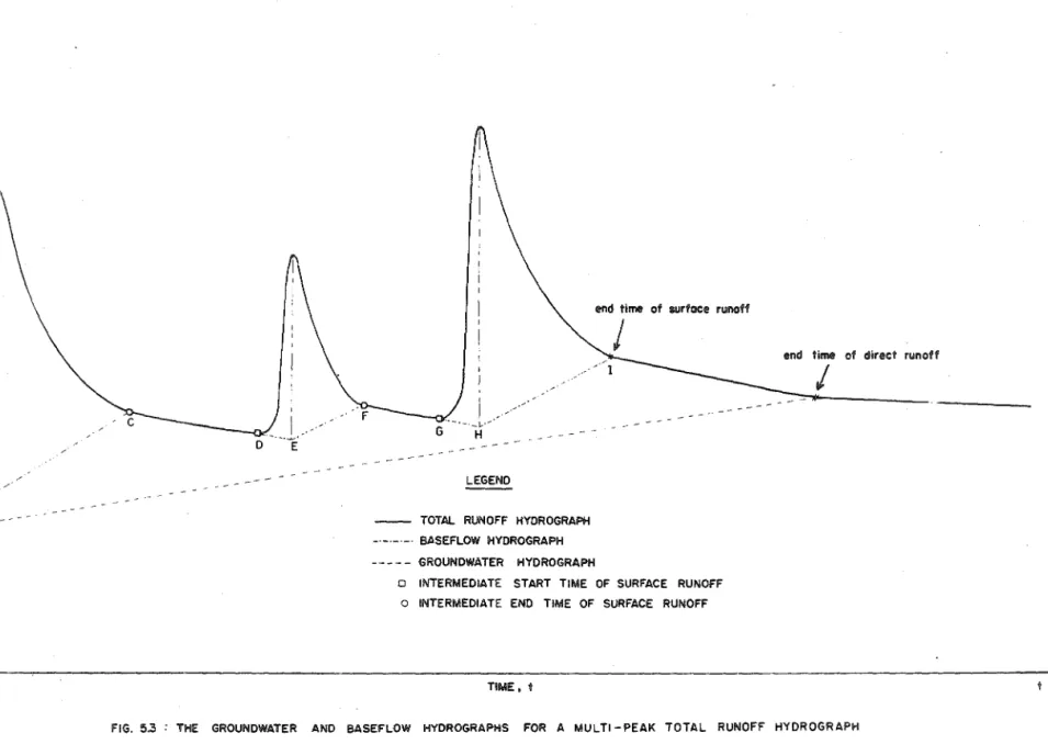
5.1.2 Time Limits of Direct Runoff
vi.
5.1.3 Time Limits of Surface Runoff 5.1.4 Surface Runoff Hydrographs 5.2 RAINFALL ANALYSIS
5.2.1 General
5.2.2 Isohyetal Maps
5.2.3 Sub-Area Rainfall Hyetographs 5.2.4 Storm Rainfall Characteristics 5.2.5 Loss Rate Derivation
5.2.6 Sub-Area Rainfall Excess Hyetographs 5.3 LAG-MEAN DISCHARGE RELATIONSHIPS
5.4 THE OPTIMISATION PROCEDURE 5.5 GOODNESS-OF-FIT CRITERIA 5..6 SENSITIVITY ANALYSIS
5.7 STATISTICAL ANALYSIS OF THE LOSS RATE 5.7.1 General
5.7.2 Principal Components Analysis 5.8 SUMMARY
CHAPTER 6. RESULTS
6.1 INITIAL ESTIMATES OF A AND B
6.2 RUNOFF ROUTING WITH THE MOTUEKA MODEL
6.2.1 Equation 3.5 Suitable for New Zealand Catchments?
6.2.2 Motueka Model Tests
6.2.3 Effects of Using Multiple Loss Rates for a Storm
6.3 SENSITIVITY ANALYSES 6.3.1 General
6.3.2 Vegetal Land Treatment 6.3.3 Mechanical Land Treatment 6.4 LOSS RATE REGRESSION ANALYSIS
Page 64 65 67 67 67 70 70 72 74 74 76 77 77 80 80 80 82 83 83 86 86 87 98 98 98 100 104 108
6.4.1 General 108
6.4.2 Loss Rate Data 108
6.4.3 The Independent Variables 109
6.4.4 Categorisation of the Storm Variables 109 6.4.5 Identification of the Components in
Table 6.7 113
6.4.6 Categorisation of the Catchment Variables 115
6.4.7 The Loss Rate Equation 119
CHAPTER 7. EVALUATION OF RESULTS
7. 1 THE MOTUEKA MODEL
7.1.1 Evaluation of Performance 7.1.2 Input Data
7.1. 3 Effects of Errors in the Locations
7.1.4 The Routed Recessions 7.1.5 Optimisation
7.1.6 Equation 3.5
7.2 THE SENSITIVITY ANALYSIS RESULTS
Reservoir 125 125 125 128 130 131 133 136 139
7.2.1 General 139
7.2.2 Suspended Sediment Quantities 140
7.2.3 Shape of the Sensitivity Analysis Curves 141
7.2.4 Influence of Catchment Storage 141
7.2.5 Mechanical Land Treatment 142
7.3 THE LOSS RATE RESULTS
7.3.1 Single vs. Multiple Loss Rates 7.3.2 Encouraging Features
7.3.3 Uncertainties With Equation 6.4 7.3.4 Further Investigation
CHAPTER 8. SUMMARY OF THE INVESTIGATION 8.1 REVIEW
8.2 CONCLUSIONS 8.3 RECOMMENDATIONS
REFERENCES
APPENDIX A. GEOLOGY AND LAND-USE DETAILS
APPENDIX B. MODEL DETAILS
APPENDIX C. COMPUTER PROGRAMS
APPENDIX D. RESULTS, STORMS AND TREATMENT LOCATIONS
MAP 1. THE MOTUEKA CATCHMENT (The fold-out at the back)
Figure 3.1 3.2 3.3 4.1 4.2 4.3 4.4 4.5 4.6 4.7 4.8 4.9 4.10 4.11 4.12 4.13 4.14 4.15 4.16 4.17 4.18 4.19 4.20 4.21 4.22 viii.
LIST OF FIGURES
A classification of prediction models - adapted from Chow (1972)
Two idealised forms of the Laurenson model Combination of initial loss and the loss rate
Location of the Motueka catchment
An upstream view from the Upper Motueka outlet
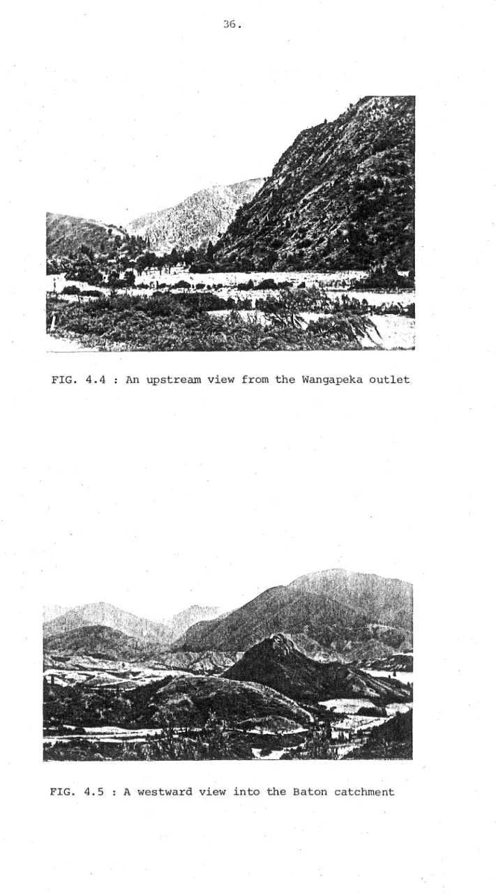
A downstream view from below the Upper Motueka outlet An upstream view from the Wangapeka outlet
A westward view into the Baton catchment
A westward view across the lower part of the Woodstock catchment
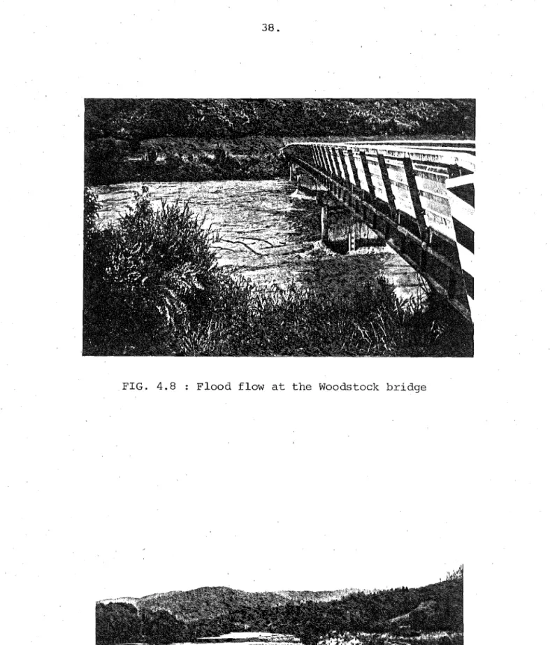
A downstream view from Woodstock Flood flow at the Woodstock bridge An upstream view towards Bluegum Corner
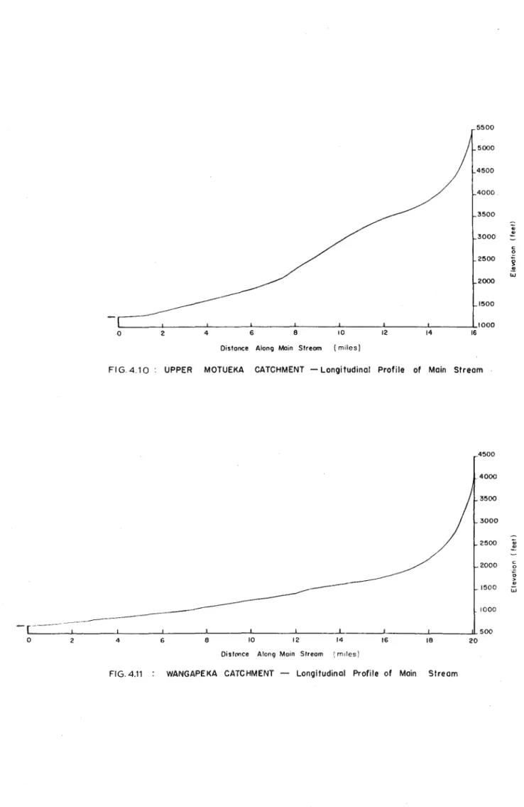
Upper Motueka catchment - Longitudinal profile of main stream
Wangapeka catchment - Longitudinal profile of main stream Baton catchment - Longitudinal profile of main stream Motueka catchment - Longitudinal profile of main stream Motueka catchment - Average annual isohyetal map
Motueka catchment - Geological classes Motueka catchment - Land uses
Motueka catchment - Rainguage locations
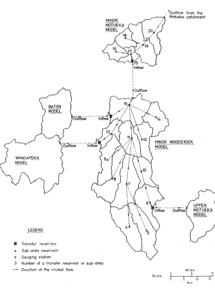
Motueka model - Composition and routing pattern
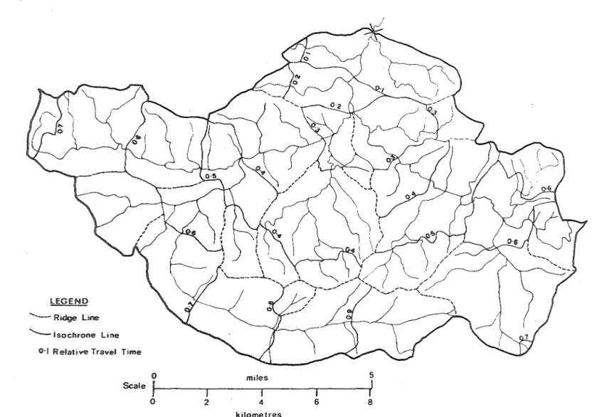
Upper Motueka catchment - Drainage pattern and modified isochronal sub-areas
Wangapeka catchment - Drainage pattern and modified isochronal sub-areas
Baton catchment - Drainage pattern and modified isochronal sub-areas
Illustration of the general routing procedure
Figure 5.1 5.2
A differentiation of streamflow components A method of obtaining surface runoff
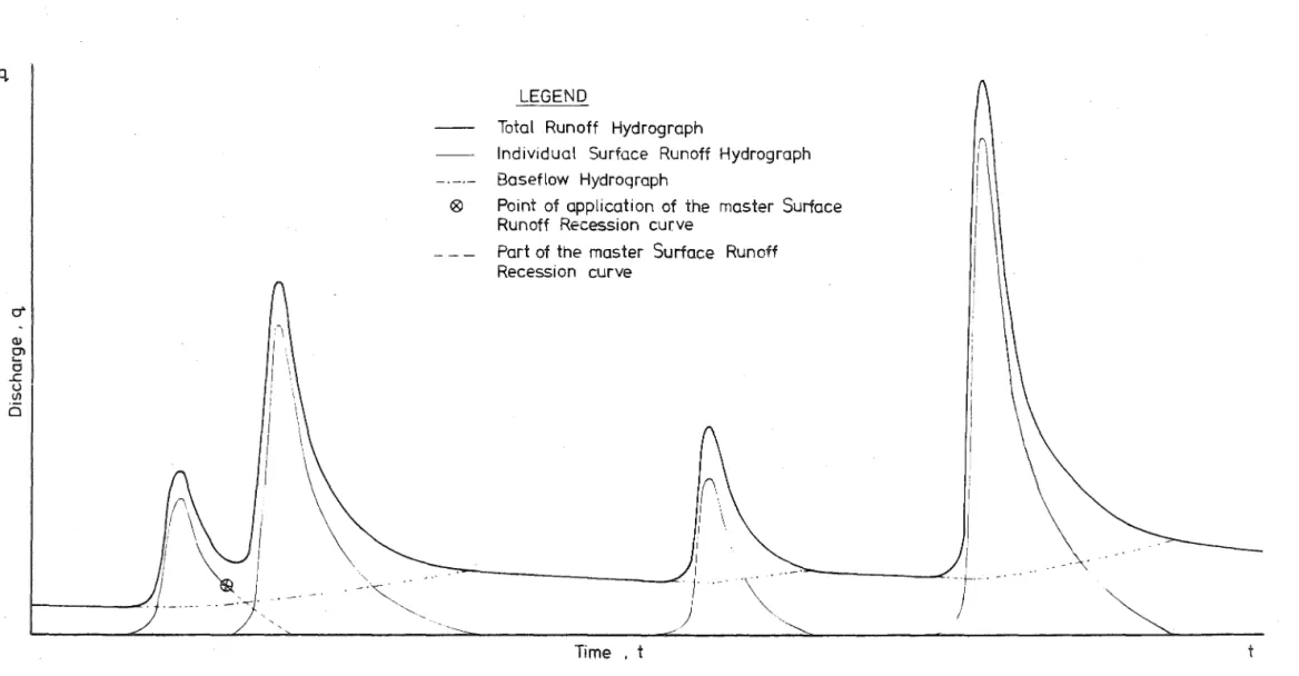
5.3 The groundwater and baseflow hydrographs for a multi-peak hydro graph
5.4 The individual surface runoff hydrographs for the multi-peak hydrograph in Figure 5.3
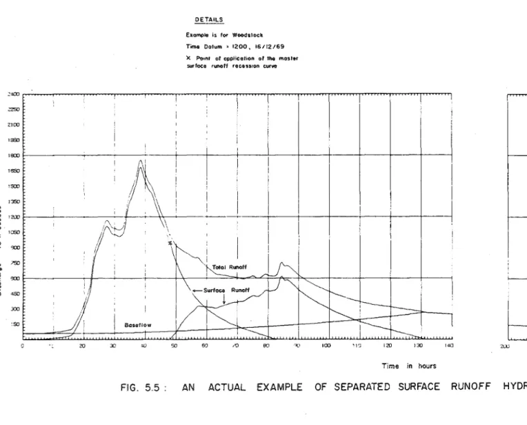
5.5 5.6 5.7
6.1
An actual example of separated surface runoff hydrographs Flow diagram of the derivation of the loss rate
Definitions of the goodness-of-fit indices
Storm No.6 - Routed hydrographs using Equation 3.5 6.2 and 6.3
6.4 and 6.5 6.6 and 6.7 6.8 and 6.9
Storm No.6 - Optimum routed hydrographs Storm No.13 - Optimum routed hydrographs Storm No.21 - Optimum routed hydrographs Storm No.24 - Optimum routed hydrographs 6.10 6.11 6.12 6.l3 6.14 6.15 6.16 6.17 7.1 7.2 7.3 7.4
Baton model and storm No.24 - Effects of using multiple loss rates
Storm No.6 - Sensitivity analysis curves for the Upper Motueka catchment
Storm No.6 - Sensitivity analysis curves for the Wangapeka catchment
Storm No.6 - Sensitivity analysis curves for the Baton catchment
Storm No.13 - Sensitivity analysis curves for the Upper Hotueka catchment
Storm No.13 - Sensitivity analysis curves for the Wangapeka catchment
Storm No.13 - Sensitivity analysis curves for the Baton catchment
Prediction of the hydrological responses to afforestation in the Baton catchment for storms No.6 and 13
Evaluation of the Motueka model Correlation of th optimum A e .
optlmum B ratio with storm size Scatter diagram for Equation 6.4
Examination of the residuals from Equation 6.4
Table
4.1 5.1 6.1
x.
LIST OF TABLES
Catchment nomenclature and associated data A differentiation of streamflow components
Correlations of catchment lag with mean discharge 6.2 Correlations of catchment lag with mean discharge
considering only the five summer storms 6.3
6.4
6.5
Details of the initial and optimum,routed surface runoff hydrographs in Figures 6.1 and 6.2
Sensitivity analysis results for the mechanical land treatment
Definitions of the regression variables 6.6 Wangapeka catchment - Matrix of correlation
coefficients from considering eight variables and
Page 39 61 84 86 90 104 110
sixteen storms III
6.7 Wangapeka catchment - The component loading matrix after Varimax rotation, from considering seven
variables and sixteen storms 112
6.8 Grouping of the storm variables 115
6.9 Correlation matrix, from considering twenty one variables,
eight storms and the five constituent catchments 117
6.10
6.11 6.12 6.13 7.1
The component loading matrix after Varimax rotation, from considering twenty variables, eight storms and the five constituent catchments
Grouping of the catchment variables
Example calculation of the loss rate using Equation 6.4 Range in the regression data sample
NOTATION Symbol
A Coefficient in the reservoir delay time-discharge equation (Eq. 3.11).
A Area of a sub-area, in square miles. s
B The exponent in the reservoir delay time-discharge equation (Eq. 3.11).
c A routing variable.
d The rainfall total of a sub-area rainfall hyetograph, in inches.
i A rate of inflow to a reservoir.
K Delay time of flow through a reservoir, in hours. k Depletion ratio constant.
r
L Catchment lag, in hours. L
t The average travel time for a catchment during a small time increment.
nr Number of sub-areas in a catchment that received rainfall.
q Used to denote streamflow discharge (e.g. Eq. 3.8) and also a rate of outflow from a reservoir (Eq. 3.12). A rate of direct runoff, in cusecs.
A rate of total runoff, in cusecs.
~D Mean rate of total runoff over the period of direct runoff, in cusecs.
~S Mean rate of total runoff over the period of surface runoff, in cusecs.
Y The abscissa value of the centroid of the dimensionless
Lit
time-area diagram.
Routing period,in hours.
LiTR The difference in relative travel time for the
reservoir concerned and the adjacent one downstream.
T Travel time from a point in a catchment to the outlet. TR Relative travel time from a point in a catchment to
the outlet.
1.
CHAPTER 1
INTRODUCTION
1.1 GENERAL
Catchment management has been defined (Hewlett and Nutter, 1969) as the management of the natural resources of a catchment primarily for the production and protection of water supplies and water-based resources, including the control of erosion and floods, and the protection of
aesthetic values associated with water. One catchment management practice is the alteration of the land use to improve the downstream water quality and quantity characteristics in a catchment. Afforestation, for example, has long been acknowledged asa major form of catchment management in stabilising soil slopes and halting accelerated erosion. There is now also recognition of its dual effect in reducing flood runoff, thereby limiting the flood risk. Alternatively, in regions where water is scarce, a change in land use from forest to grass can be an effective measure in increasing water yields while still maintaining soil stability.
The 1416 square mile (3667 km2) Waimakariri catchment on the eastern slopes of the Southern Alps in New Zealand has a flood problem. A committee was formed to investigate the likely effects of various land treatments, including the possible afforestation of the whole of the upper catchment to the 3000 ft (915 m) level, in terms of changes at the catchment outlet to water yield, flood peak discharges and water quality. No
The possible Waimakariri scheme typifies the types of "physical forecasting" requests that can be made. With an increasing number of similar catchments likely to come under similar scrutiny, there is a clear need for a method which will assist in the prediction of the hydrological effects of land-use changes.
1.2 PREDICTING EFFECTS OF LAND-USE CHANGES
Previous work (see Chapter 2) has made the prediction of the
qualitative effects of land-use changes on the flood hydrograph reasonably straightforward. The difficulty is in quantifying the effects. With the work cited in Chapter 2, the quantitative effects of given land-use changes varied with the catchment studied.
One of the causes of the varying responses is the varying hydrologica size of the catchments studied. A hydrologically small catchment is one with runoff characteristics primarily determined by the factors which govern
overland flow, e.g. high-intensity rainfalls and land use, In hydrologically large catchments the catchment storage is the predominant factor governing the streamflow. It attenuates and translates the flood hydrograph,
largely suppressing the effects of land-use changes on the hydrograph shape and peak. The physiography of a catchment, which governs its storage
capacity and therefore its ability to mask the effects of land-use changes, uniquely defines each catchment. This uniqueness suggests that each
catchment's flood hydrograph response to land-use changes is different and the evidence to date supports this view.
The matter is further complicated by the actual location of the
3.
each site located differently in relation to the drainage pattern and, therefore, with respect to the distribution of catchment storage. Hence, one site may exhibit greater sensitivity, in terms of changes in the flood hydrograph characteristics, than another to treatment.
The flood hydrograph response to land treatment depends then, not only on the particular catchment, but also on the location of the treatment within the catchment. The catchment concerned and the particular land treatment site together produce a unique set of storage characteristics. Each problem concerning the effects of land-use changes on the flood hydrograph therefore demands its own individual solution.
1,3 PREDICTION TECHNIQUES
The earliest form of prediction of the effects of land-use changes involved the translation of the observed effects of similar changes in a similar catchment, However, physical similarity does not always imply hydrological similarity. Indeed Lull and Sopper (1967) found there was as much variation between catchments within a physiographical region as there was between regions.
A more objective approach is the use of multiple regression analysis e.g, Anderson (1949), Based on an analysis of experimental data a dependent variable, often flood peak discharge, is mathematically related to a set of independent variables. The latter will include those variables deemed relevant by the researcher. The effect of a land-use change is deduced by altering one or more of the independent variables.
be involved, While the resulting equation can be statistically significant it may give misleading cause and effect relationships. There is also some doubt as to whether it can be applied to other catchments.
Neither of the above prediction techniques, in common with some more elaborate ones e.g. regional analysis (Storey et aI, 1964), can properly take into consideration the land treatment location. They therefore
inadequately account for the effects of catchment storage. A more satis-factory prediction method would be one which actually simulates the catchmeni storage effect. Numerous models have been developed to do this in either physical or mathematical form. A description of such models appears in Chapter 3. They all require a land-use parameter which is altered to simulate land~use changes. often a lack of information prevents the quantitative expression of changes in land use by such a parameter. In these cases the sensitivity analysis technique described below appeals as a satisfactory alternative.
1.4 SENSITIVITY ANALYSIS TEC~NIQUE
The sensitivity analysis technique, of the type proposed by
Burton (1969), is a method for evaluating the hydrological sensitivity of different parts of a catchment to land-use changes, It uses a model whose structure is based on the sub-areas of a catchment and incorporates paramete that are meaningful and measurable land-use indices for the sub-areas.
5.
The advantage of this technique is that no specific numerical values are required to determine the sensitivity of the various sub-areas. If the sub-area under investigation is found to be sensitive to changes in the land-use index, then an examination of the values of the changes is necessary. Detailed information about the change in land-use index following the proposed treatment is then required.
1.5 TBE PRESENT INVESTIGATION
A method was sought which could be used for any catchment to predict the effects of land-use changes on the flood peak and the quantity of
suspended sediment transported in a flood, It was essential that the
metho~ simulated the catchment storage effect and incorporated the
sensitivity analysis technique. Obtaining a relationship between the method's land-use index and different land uses was a desirable but less important objective.
With afforestation being the most popular form of land treatment in large catchments in New Zealand it was taken as the principal form of land-use change in this study.
CHAPTER 2
SOME HYDROLOGICAL EFFECTS OE' CHANGES IN FOREST COVER
The effects of forests on floods and suspended sediment are reviewed in Sections 2.1 and 2.2, respectively. The effects are then summarised in Section 2.3.
2.1 FORESTS AND FLOODS
2.1.1 Increase in Forest Cover
Forests promote infiltration, i.e. the entry of water into the soil through the ground surface. They achieve this in the following ways.
(a) The root system maintains a relatively stable and porous soil structure (b) The litter cover and the leaf mould protect the soil from compaction
by raindrops.
(c) The litter cover also retards any overland flow and hinders the surface sealing of soil pores.
(d) Evapotranspiration, which depends on the climate and the depth of the root zone, causes soil moisture deficiencies and so increases the potential for infiltration.
Lull and Reinhart (1972) report that in mature forest infiltration is seldom limiting: infiltration rates generally exceed rainfall intensities so that overland flow is virtually absent. They also point out that the surface runoff (defined in Section 5.1.1) from a forested catchment is due almost entirely to subsurface flow. The infiltrating water moves rapidly to the stream channels through the large voids in the topsoil which have been
7.
The net result of forests promoting infiltration and providing greater opportunity for soil moisture storage is a reduction in surface runoff. Consequently, flood peak discharges are also reduced. According to Lull (1971), afforestation of eroding land can reduce peak discharges by up to 60 to 90 percent.
However, the reduction in peak discharge with increase in forest cover has been found to be extremely variable and is dependent on many factors. The reduction depends on the proportion of a catchment forested (Lull and Reinhart, 1972). It also depends on the climate and the season, since these factors affect evapotranspiration and thus the opportunity for soil moisture storage. For instance, in winter the opportunity for infiltrating water to be stored or detained in the soil is less than that in the summer, when evapotranspiration is greater and the soil moisture deficit is corres-pondingly higher. Hence, peak discharge reductions are usually higher in summer than in winter. In the White Hollow catchment, a Tennessee Valley Authority (TVA) catchment of 1715 acres (6.94 km2), improvement in forest cover over a 24 year period reduced summer peak discharges by about 80 percent (Ellersten, 1968). The reductions for the winter storms were much
less, ranging from 0 to 28 percent.
Further, the reduction in peak discharge depends on the magnitude of the storm. In the large storm the proportion of the infiltrating water stored or detained in the soil will normally be less than that for the small storm. Thus the peak discharge reduction will generally be less significant in the large storm (Kittredge, 1948; Leopold, 1970).
Nevertheless, the reduction in peak discharge in a large storm can be substantial. Pereira (1973) reports of a large storm in Kenya on land
rain fell in one hour during the storm, and the peak rainfall intensity was approximately 10 in/hr (250 mm/hrJ. Despite these extreme rainfall conditions, the peak discharge per unit area for a cleared and cultivated catchment was more than forty times greater than that for a nearby,
forested catchment.
The depth of soil is another factor that affects the reduction in peak disCharge. With shallow soils over impermeable rock the initial infiltration rate is still high, but rapid saturation of the soil occurs. Thus the forest on a shallow soil can delay the onset of surface runoff, but its control over surface runoff and the peak discharge diminishes in a prolonged storm where the foliage, litter cover and the soil all
become saturated. For example, in a low-intensity storm in the Appalachian mountains where 8 inches (203 mm) of rain fell on wet, forested catchments, the peal~ discharge per unit area for a catchment with only a 2 foot (0.6 m) depth of soil was more than five times that for a catchment where the soil was 6 feet (1.8 m) deep (Hursh, 1943).
In addition to the factors already mentioned, the reduction in peak discharge depends on the catchment storage and the location of the forest cover increase, for the reasons given in Section 1.2. These two factors have not always been properly accounted for in research, and the latter one especially has not been closely examined. Lull and Reinhart (1972) have noted, though, a tendency for the forest influence in reducing the flood peak to diminish with increasing catchment size.
9.
most of the precipitation occurs as snow and the major runoff events each year are due to snowmelt. For these conditions it has also been observed that forests transform the runoff pattern. From a summary of a century of Russian observations and opinions, Molchanov (1963) concluded that when a catchment is selectively forested, to 30-40 percent of its area, all overland flow is transferred to the subsoil. Sokolovsky (1959) indicated that the reductions in overland flow and the subsequent recharge of
groundwater caused low flows to increase three to five times.
The reductions in overland flow are again the result of forests improving the conditions for infiltration. Forests lessen the freezing of the soil, and also provide a longer time for infiltration by delaying and attenuating the snowmelt.
This latter effect is due to the forest intercepting radiation and desynchronising the snowmelt in different parts of a catchment. Sozykin
(1959) noted that the melting of snow takes approximately twice as long in forests as it does in open areas, while Goodell (1959) found that snow in unshaded forest openings melts 20 to 30 percent faster than snow shaded by forest.
Boughton (1970) concluded that, because of the delay and attentuatior effect on snowmelt, forests can significantly reduce peak flows in large catchments where snowmelt is the principal flood-producing factor.
2.1.2 Decrease in Forest Cover
When the forest cover in a catchment is reduced the effects are the converse of those produced by afforestation, i.e. surface runoff and peak discharges are increased (e.g. Nakano, 1967). Further, because the difference in soil moisture deficits between forested and deforested catchments is
generally greater in summer, the increases are usually higher in the summer. 2
In a deforestation experiment on a 39.5 acre (0.16 km ) catchment in New Hampshire, USA, Hornbeck (1973) observed that by far the greatest increases in direct runoff (surface runoff plus interflow) and peak flows occurred during the summer season. Over the period of the experiment the greatest increases in direct runoff and peak discharge, of two and threefold
respectively, occurred in a summer storm when there was a large soil moisture deficit in the forested control catchment.
The method of removing the forest cover affects the streamflow increases. Provided the AO and Al horizons of the soil are well developed and essentially undisturbed after forest removal, the increases can be minimal (Kittredge, 1948). For example, with forest cutting alone, the remaining vegetation may sometimes be as effective as the uncut forest in minimising surface runoff and peak discharges (e.g. Hewlett and Hibbert,
1961) .
In comparison, logging and fire are much more drastic forms of
11.
Reforestation of a deforested catchment rapidly reduces the
surface runoff and peak discharges (Leopold, 1970). In the White Hollow catchment (see Section 2.1.1) the peak discharge reductions of about 80 percent were achieved within the first two or three years after the reforestation. Further, the results (Hibbert, 1967) of water yield studies at Coweeta, North Carolina, give an indication that after reforestation the streamflow variables return almost to their original values.
2.2 FORESTS AND SUSPENDED SEDIMENT
Afforestation of eroding land sharply curbs erosion and reduces the quantity of suspended sediment. For example, with land in Mississippi where erosion had removed the equivalent depth of two feet (0.6 m) of soil, afforestation reduced the annual soil loss rate from several tons/acre to 0.00-0.08 tons/acre (Ursic and Dendy, 1965). And in two TVA catchments, the White Hollow catchment and the 88 acre (0.35 km2) Pine Tree Branch catchment, improved forest cover on eroding land contributed to a
lowering in the annual sediment load of 96 and 98 percent, respectively (Ellersten, 1968).
Afforestation reduces the quantity of suspended sediment through the following mechanisms:
(a) by decreasing overland flow and surface runoff (Section 2.1.1) I and therefore the sediment transporting capacity;
(b) by protecting the soil against raindrop action, by decreasing the detaching energy of the raindrops and the detachability of the soil particles (Osborn, 1955);
(e) by increasing the deep-seated land stability, by the mechanical reinforcement from the root system and by the alteration of the soil moisture regime.
The decrease in overland flow (mechanism a) reduces the number of particles transported to the river system, while the decrease in surface runoff (also mechanism a) reduces the quantity of sediment transported by the river itself. Since the sediment transporting capacity of a river increases at the rate of the second or third power of its velocity a decrease in surface runoff, which is usually accompanied by decreased
river velocities, may reduce the sediment load considerably. The reduction is magnified by the remaining four mechanisms, which restrict the source and supply of sediment.
Because forests reduce surface runoff and the quantity of suspended sediment they act as a control on floods. They decrease peak discharges and also decelerate the downstream riverbed aggradation.
Forests also maintain a high water quality. The water from catch-ments in well-established forest characteristically contains very low suspended sediment amounts, except in times of infrequent high flows
(Packer, 1967; Lull and Reinhart, 1972).
However, removal of the forest cover reverses the mechanisms listed earlier and noticeably increases the quantity of suspended sediment. As with streamflow, the most dramatic increases follow deforestation by logging
l3.
2.3 SUMMARY
Outstanding characteristics of forests are their promotion of infiltration, their increasing of the soil moisture storage capacity, and their physical effect in stabilising the soil. As a consequence of the first two characteristics, afforestation reduces overland flow, surface runoff and peak discharges. The combination of the three characteristics causes a marked decline in the quantity of suspended sediment. with deforestation, the reverse effects occur.
Although these effects of changes in forest cover are qualitatively consistent, quantitatively they are highly variable and are therefore difficult to predict. For instance, the reduction in peak discharge following afforestation varies according to the extent of the treatment, the climate, the season, the storm and the soil conditions. In a prediction these factors can be handled satisfactorily by a multiple regression
equation. What cannot be handled so easily is the fact that the reduction in peak discharge also depends on the catchment storage and the treatment location - two factors which have not always been given due recognition in research.
The reduction in the suspended sediment quantity following
afforestation is also dependent on these two factors, since the quantity is influenced by the river discharge as well as by the soil stability.
Because this investigation was concerned with the development of a method for predicting the effects of land treatment on peak discharge and the quantity of suspended sediment transported in a flood, emphasis was placed on accounting for these factors of catchment storage and the
study was afforestation, the problems posed by catchment storage and the treatment location are the same whatever the form of land treatment.
Simulation was considered the most satisfactory way of accounting for the two factors. The model that was used in the simUlation is
14.
CHAPTER 3
SELECTION OF A MODEL
The Laurenson model was selected for use in this investigation and it is described in Section 3.4. The description is preceded by a list of the selection criteria (Section 3.1), a general classification of relevant prediction models (Section 3.2) and comments on individual models (Section 3.3). In the last section (3,5) the Laurenson model's loss rate parameter is explained and then justified as a suitable land-use index for a
sensitivity analysis.
3,1 OBJECTIVE AND REQUIREMENTS OF THE MODEL
A prerequisite for an accurate prediction of land treatment effects on the flood peak and the quantity of suspended sediment transported in a flood is a satisfactory reproduction of the flood hydrograph. With this as the chosen objective of the model sought, it was important that the model should have the following attributes.
(a) Applicability to hydrologically small and large catchments alike, i,e. the catchment storage effect should be simUlated.
(b) Structural facility for a sensitivity analysis, i,e. the model should contain sub~areas.
(c) A physically meaningful and measurable parameter that would serve as the land-use index in the sensitivity analysis.
3.2 A CLASSIFICATION OF MODELS
Models that can be applied to predict the hydrological effects of land treatment can be classified according to an adaptation of Chow's
(1972) system (see Figure 3.1).
The physical models resemble or imitate the major hydrological processes within the catchment. Their division into scale, analogue and simulation models, respectively, depends on whether:
(a) the model is a reduced physical replica;
(b) the behaviour of the model's components are analogous, in a mathematical sense, to the hydrological processes; or
(c) the model is in digital form.
With the abstract model there is no attempt to model the hydrologicaJ processes exactly. Instead the processes are replaced by a set of
mathematical relationships that approximate the catchment's runoff behaviour
The lumped form of abstract model may be linear or non-linear. It treats the catchment as a single point in space without dimensions and assumes homogeneity of the input data and homogeneous catchment conditions. On the other hand, the distributed model considers the runoff behaviour within the catchment, so that its mathematical formulation contains space dimensions.
SCAlE
( e.g.Chery. 1966)
PHYSICAL
ANALOGUE
(e.g. Riley et 01 , 1968)
CATCHMENT MODELS
,
ABSTRACT
SIMULATION
(e.g. Crawford and Linsley, 1966)
DISTRIBUTED
(e.g. Wooding ,1965,66)
LUMPED
( CONGLOMERATED LUMPED)
LINEAR NON-Ui'EAR (e.g. Shultz, (e.g. Laurenson,
1968) 1962)
FIG. 3.1: A CLASSIFICATION OF PREDICTION MODELS - Adapted from Chow (1972)
}--'
3.3 WHICH MODEL? 3.3.1 General
The criteria for selecting a model were the objective and requirements in Section 3.1.
Neither analogue nor physical models were seriously considered because both lack generality. Moreover, physical models require extensive field data and are susceptible to similarity problems.
The different models that were considered are mentioned below.
3.3.2 Simulation Models
The Stanford Watershed model (Crawford and Linsley, 1966) simulates the basic processes of the land phase of the hydrological cycle. It has been used to study effects of land-use changes (e.g. Fleming, 1971) but was inappropriate in this present situation because of:
(a) the extensive data demands for each sub-area - information on over twenty parameters is required;
(b) the natural tendency, as a consequence of point (a), to use a minimal number of sub-areas;
(c) the uncertainty over a suitable land-use index.
18.
This was a finding with the Dawdy and O'Donnell (1965) model. The model is a water balance approach like the Stanford model, but less
sophisticated, and it was designed primarily to test optimisation techniques. Because of the ease with which parameter values could be fitted, the
techniques were seen to permit refinements of a model by encouraging the addition of more parameters. It was concluded, however, that while
refinements may improve a model's performance the optimum parameter values may reflect reality less and less. The same warning on the potential abuse of optimisation techniques was reiterated by Kane et al (1973).
While containing fewer components than the Stanford model, the
Boughton (1965, 1968a) model is proving a useful tool in water yield problems and improvements by Jones (1969) and Taylor (1971) have enhanced its
reputation in this field. The model works on daily surface runoff volumes, though it was modified later (Chapman, 1968, 1970) to operate on shorter time intervals.
Another prominent simulation model is the USDAHL-70 model (Holtan and Lopez, 1971), and it has been applied to evaluate effects of land-use changes, e.g. Glymph et al (1971). The model differs from those previously mentioned in that no optimisation technique is used. The output is computed from predetermined, specific values for the different parameters. This requires extensive field data.
3.3.3 Distributed Models
Despite improvements by Woo1hiser, in association with others
(Woolhiser et al , 1970; Kibler and Woolhiser, 1970; smith and Woolhiser, 1971), the Wooding-type model appears limited in its use by its emphasis on overland flow, which is not the major factor influencing the streamflow of a large, rural catchment.
3.3.4 Conglomerated Lumped Models 3.3.4.1 Catchment storage
In a conglomerated lumped model the rainfall excess is routed, according to a concept of the runoff process, through a representation of catchment storage that involves sub-areas. The catchment storage can be represented by concentrated and distributed storages. The two types of storage are differentiated by their dominant effect on a hydrograph. Although both types attenuate and translate a hydrograph, the former effect is principally associated with a concentrated storage (e.g. a reservoir) and the latter with a distributed storage (e.g. a channel).
Laurenson (1962) showed the futility of separating the effects of the two types of storage in a model. A series of concentrated storages was found to simUlate both the attenuation and translation effects.
3.3.4.2 Non-Linear Models
Catchment streamflow exhibits a non-linear response to rainfall input. This was shown in studies by Singh (1962), Diskin (1964),
20.
warrant non-linear considerations, only the non-linear models were considered.
In his model of the Columbia Basin Rockwood (1958) used non-linear reservoirs to represent lake, channel and catchment storages. The combinatic' of reservoirs resembled the hydrological structure of the Basin.
The Laurenson (1962) model, shown in two idealised forms in Figure 3.2, has greater flexibility and simulates the response of a catchment as a whole, rather than distinguishing between the responses of the land and channel components. The model considers sub-areas of a catchment and a non-linear reservoir at the centre/centroid of each, The rainfall excess
for each sub-area is assumed spatially uniform and concentrated at the location of the reservoir.
The rainfall excess for a sub-area is converted to an equivalent hydrograph, combined with the routed outflow from the adjacent, upstream reservoir(s), and then routed through the reservoir in the sub-area
concerned. Repetition of this process down to the catchment outlet produces the surface runoff hydrograph. In operating in this manner the Laurenson model allows for:
(a) spatial (between sub-areas) and temporal variations in rainfall excess; (b) rainfall excesses from different parts of the catchment passing
through different amounts of catchment storage,
(c) catchment storage being distributed rather than concentrated; (d) non-linear catchment behaviour, i,e. the non-linear relationship
Relative Travel Times
lsochrones
FIG.3.2a ISOCHRONAL SUB-AREA APPROACH
I
Sub - ea tehment boundary I_--""'C"~:
( Ridge line)
I
I
,
,.-IFIG.3.2b SUB-CATCHMENT SUB-AREA APPROACH
0·8
Non -linear Concentrate! Storages or Reservoirs
22.
For these reasons it was decided to use the Laurenson model. A fuller description of the model follows,
3.4 THE LAURENSON MODEL 3,4.1 Structure
The Laurenson model requires the catchment to be divided into sub-areas, each containing a non-linear reservoir. The division into sub-areas can be done in any reasonable way. In the most common form of the model, the isochronal approach (Figure 3.2a), the sub~areas are defined by isochrones, i,e. lines of equal relative travel time (see Section 3.4.2), and the reservoirs are located at the sub-area centres, i,e, halfway between the isochrones.
In a second and less promoted form of the Laurenson model, the catchment approach (Figure 3.2b), the areas are defined by sub-catchment boundaries and the reservoirs are located at the centroids of the sub-areas, This modelling approach achieves a closer approximation of the drainage system. The advantages of the sub-catchment approach are:
(a) the time spent in constructing the model is much less; and
(b) the sub-division of the model is more adaptable and meaningful for land treatment problems than the imaginary isochronal sub-areas.
The sub~catchment approach is virtually untested; in its sole trial by Laurenson (1962) it performed less creditably than the isochronal approach, On the basis of its practical advantages alone it was considered worthy of further research.
3.4.2 Travel Time
is required to know the travel time of flow from each reservoir to the catchment outlet, as explained later in Section 3.4.4. Laurenson rejected the drop-of-water concept in considering travel time. He treated the
travel time for a point in the catchment as the time between the occurrence of an element of rainfall excess at the point and the effect of this element at the outlet. The complication in treating travel times in this more
realistic fashion is that the times then depend on the discharge. It
is therefore convenient to obtain the travel times for the reservoirs initiaJ.I in dimensionless form, expressing them in relation to the maximum travel timE' for a point in the catchment. The relative travel times can later be made dimensional when the travel time is determined for a point in the catchment with which other points can be associated.
Relative travel times for points in a catchment are calculated on the premise that the travel time of flow from a point along the point's flow path to the outlet is proportion to
~l/S~i
where 1 is the length of flow path between a pair of adjacent contours, S is the slope of the correspondin(~ reach, and the summation is performed along the flow path from the point to the outlet. Travel times calculated in this way are then made relative to the maximum time calculated for the catchment.In the isochronal approach the relative travel times for the reservoirs are obtained by determining dimensionless isochrones (see
Figure 3.2a)and then placing the reservoirs halfway between the isochrones. In order to obtain the isochrones relative travel times must be calculated for a large number (200-600) of points in the catchment,
24.
relative travel times for the reservoir location points.
3.4.3 Catchment Lag
Catchment lag provides the link between travel time and discharge. It is defined as the difference in time between the centroids of the
catchment rainfall excess and the resulting surface runoff hydrograph. In effect, catchment lag is the average travel time for all points in the catchment, where the averaging is done throughout the duration of the storm.
Laurenson showed that, for a small increment of time and for spatially uniform rainfall excess, the average travel time Lt was equal to
0-the abscissa of 0-the centroid of 0-the dimensio~~ time-area diagram. Thus the travel time L for a point may be expressed as
. . . . , • • • , . . 0 3.1
where the corresponding relative travel time;
and Y
=
the abscissa value of the centroid of the dimensionless time-area diagram.In fact the time~area diagram is not required to obtain Yi Y can be calculated from
ns
2: A LR
i=l s
Y := ., v " .. 0 • 9 <I Q q 3.2
ns ,2: A
1=1 s
where As := area of a sub ... area
LR ;::: the relative travel time for the reservoir in the sub-area;
To explain how L
t in Equation 3.1 varied with discharge Laurenson examined the behaviour of the time-average value of Lt, the catchment lag L. From an analysis of twenty three storms he established the following
relationship for the 35 square mile (90 km2) South Creek catchment in New South Wales.
L ::::: 64qT -0.27 3.3
"
...
"",,""" "where L ::::: catchment lag, in hours;
and ~ :::: mean rate of total runoff over the period of surface runoff, in cusecs.
In a similar but more detailed study, Askew (1968a,b) found that the correlation between the two variables improved if a weighted mean discharge qTD was considered, where
-where qTD :::;
qD ;:::
qT :=: and n ::::
ndl
E
qi:::::l D
weighted mean rate of total runoff (surface runoff plus a regularly spaced ordinate the corresponding ordinate the number of ordinates of
" " .... " , " " .... 3" 4
runoff over the period of direct interflow) ;
of direct runoff; of total runoff; direct runoff.
26.
L 5 64AO. 541S -0.16-. c s qTD -0.23 . . . 3.5
where qTD is in cusecs, Acis the catchment area in square miles and Ss is a dimensionless overland slope factor. S is determined by overlaying a
s
square grid of lines onto a contour map of the catchment and applying the formula
S ::::: Nh ,."",,
..
,,' " 3,6s L g
where N ::::: the number of intersections of grid lines with contours; h the contour interval;
and L ::::: the total length of the grid lines within the catchment,
g
It will be noted that the general form of the lag-mean discharge relationships derived by Laurenson and Askew is
- -B
L :::l Aq
where q is some form of mean discharge and A and B are positive constants.
Although A and B in Equation 3,7 relate to time-average values of lag and discharge, Laurenson assumed that they could also be applied to the instantaneous. values of the two variables. Hence
-B
Aq
where q is an instantaneous rate of runoff.
lR -B
l
=
- A q Y3.4.4 Routing
Inflow to each reservoir in the Laurenson model is routed according to the non-linear storage function
S ;::: K(q) .q ., .. , . . . 3.10
where S ;::: a volume of storage I
and K
=
the delay time of flow through the reservoir - it is a function of the outflow discharge q from the reservoir.The delay time K through a reservoir accounts for the travel time of the flow in the model flow reach between the reservoir and the next one downstream. It is equal to the difference in the travel time for the two reservoirs. Thus, from Equation 3.9,
K
tn
R -B
- A q
Y , ... 3.11
where 6l
R
=
the difference in the relative travel time for the two reservoir'<The routing procedure itself involves the iterative solution, for each routing period, of the following Muskingum-type equation, which is obtained from storage continuity considerations and Equation 3.10.
where subscripts 1 and 2 refer, respectively, to the start and end of the routing period, of duration 6t, and where
and
a
=
b 6tc
=
6lR -B
= - A q Y 1
28.
....•... 3.13
...••.. 3.14
...•.... 3.15
, " . , .. " . "" 3.16
Equations 3,15 and 3.16 are discrete forms of the general reservoir delay time-discharge relationship (Eq. 3.11). It can be observed from
these equations that the lag or delay time characteristics of each reservoir are like those of the catchment as a whole, i.e. each reservoir's delay time depends on the constants A and B, This assumption appears reasonable for catchments of small or moderate size. However, in a large catchment with marked spatial variations in topography it would be more realistic
to divide the catchment into smaller ones, according to the available gauging stations,and model each smaller catchment separately. The overall model would then consist of a number of separate models.
3.5 LOSS RATE 3.5.1 General
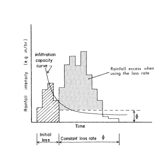
The rainfall excess in the Laurenson model is derived by applying a loss rate (~ index) to the storm rainfall. The loss rate is the average
rate at which rainfall is lost to surface runoff through being abstracted by infiltration, evapotranspiration, interception, depression and detention storage. Since these hydrological processes depend on the soil and cover characteristics (as well as the topographical and storm characteristics) , the loss rate is an index of the effect of the land use on the surface runoff hydrograph. It is therefore a convenient model parameter for expressing the effects of land-use changes.
A disadvantage with the loss rate though is that its use incorrectly implies that the rate of rainfall loss remains constant throughout a storm. Some consideration was therefore given to using a more theoretically
acceptable, available method of deriving the rainfall excess. However, the alternative methods available were rejected, because of their unsuitability of application or their lack of a suitable land-use index (Section 3.5.2).
3.5.2 Alternative Methods of Deriving Rainfall Excess
Methods that derive rainfall excess are based on infiltration theory_ This follows since rainfall excess is that part of the rainfall that appearE as surface runoff, and infiltration is the major land-based hydrological process influencing the amount and distribution of surface runoff.
The infiltration equations developed by Horton (1939), Philip (1957) and Holtan (1961) describe the infiltration capacity of a soil-cover comple~
30.
by plot experiments. However, with these experiments there are considerablE practical difficulties in obtaining data representative of a large area. This is because of the variability of soil properties, both in the vertical profile and in spatial extent. Further, account has yet to be taken in these experiments of the effects of different cover on the antecedent soil moisture conditions, the factor which governs the starting point of the infiltration capacity curve, Accordingly, there is little justification for applying infiltration theory based on plot data to whole catchments. Nor is there validity in using plot data to explain effects of land-use changes in a catchment (Boughton, 1970).
Alternatively, rainfall excess can be derived by fitting an infiltration equation to the concurrent rainfall-runoff record (Musgrave and Holtan, 1964) or by optimising the equation's parameters, e.g. as in Boughton's model (Boughton, 1968b), However, the former approach is unwieldy, and is unsuited for taking spatial variations in rainfall
intensity into account, With the latter approach there is the possibility of obtaining a physically meaningless parameter value.
In contrast, the loss rate approach can satisfactorily handle spatial variations in rainfall intensity (Horton, 1937; Laurenson, 1954) and the loss rate value is always a representative index of the catchment's infiltration rate. The loss rate method was therefore retained in this study to derive the rainfall excess in the Laurenson model.
3.5,3 Initial Loss
as initial loss and excluded from the loss rate calculations. The combination of initial loss followed by a constant loss rate often approximates the infiltration capacity curve (see Figure 3.3). The approximation works best for the major flood-producing storms on a saturated catchment, and for the storms of sufficient duration and
intensity such that the infiltration capacity has reached a near-constant rate early on in the storm. In the more moderate storms the loss rate is very dependent on the antecedent wetness conditions.
3.5.4 Variables Affecting the Loss Rate
Boughton (1970) suggested that loss rates may be insensitive indicators of land-use because of averaging effects in their derivation. However, the literature reviewed (Chapter 2) supported the loss rate-land use idea; the very definite manner in which afforestation promotes
infiltration and reduces surface runoff indicated a noticeable increase in loss rate.
The other variables, besides land use and catchment wetness, that influence infiltration can also be expected to affect the loss rate. As indicated in Chapter 2 and mentioned by Linsley et al (1958) and/or Laurenson (1967), these variables include the soil type, the intensity and duration of the storm and the temperature.
If)
C <U
-
Co
-
co
0:::
infiltration capacity
~Initial
loss
32.
, ... .
...
... ... ....
...
... ... , .. ,
.... , .... .
... '" ... .
• • • • 0 • • • • •
... ... ... .
.. , ... .
... ... ... . ,., ... .
... ... ... .
• 0 • • • • • • • • • • • •
... ... ... .
... ... ... .
t • • • • • • • • • • • • •
... ... ... .. ,
• • • • 0 • • • • • • • • • 0 . '
• • • ' 0 ' • • • • • • . • . • ,
... ,
••• '0 • • • • • • • • • • • •
... "
• • • • • • • • • • • • • • ' 0 '
Rainfall excess when using the loss rate
- - - _
... _-Time
I
Constant loss rate)0<
CHAPTER 4
THE CATCHMENT AND ITS MODEL
The principles of the Laurenson model were applied to the Motueka catchment, producing the Motueka model. Descriptions of the catchment and its model follow in Sections 4.1 and 4.2, respectively.
4.1 THE MOTUEKA CATCHMENT 4.1.1 General Description
The 780 square mile (2020 km2) Motueka catchment is situated at the north-west end of New Zealand's South Island (see Figure 4.1). It comprises such contrasting features as rugged, mountainous sub-catchments and flat, alluvial plains, with the relief ranging from sea level to approximately 6000 ft (1730 m). An impression of the general topography and drainage system can be gained from Map 1 (the fold-out at the end of the text) and from Figures 4.2-4.9,
Five gauging stations divide the catchment into five constituent catchnlents, namely the Upper Motueka, Wangapeka, Baton, Minor Woodstock and Minor Motueka catchments. The nomenclature adopted for the various parts of the catchment is summarised in Table 4.1.
Throughout this text the term true catchment refers to the total catchment area above the gauging station of the catchment
concerned. A minor catchment is not a true catchment. It is the residual catchment area after the upstream constituent catchments have been
40"
MOTUEKA
CATCHMENT
34.
42
0- - - --~---+---+-t---I---I _ _ _ _
44
0---
.-...".,=.~-+--~t---_r--t__---_FIG. 4.2
FIG. 4.3
An upstream view from the Upper Motueka outlet
36.
FIG. 4.4 An upstream view from the Wangapeka outlet
FIG. 4.6 A westward view across the lower part of the woodstock catchment
38.
FIG. 4.8 Flood flow at the Woodstock bridge
TABLE 4.1
CATCHMENT NOMENCLATURE AND ASSOCIATED DATA
Area Main Channel
Length Average
Catchment Gauging Station Channel
Miles 2 km2 Miles km Slope,%
Upper Motueka Motueka Gorge 63.74 165.1 16.00 25.75 3.13 Wangapeka Nettleton's 132.70 343.7 20.30 32.67 1. 32
Baton Faulkner's 68.90 178.5 10.85 17.46 3.36
Minor Woodstock Woodstock 410.13 1062.2
-
-
-Woodstock Woodstock 675.47 1749.5 48.08 77.38 0.548 Minor Motueka B1uegum Corner 104.71 271. 2
-
-
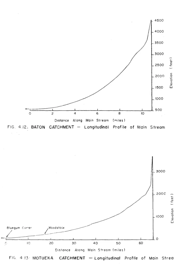
-Motueka Bluegum Corner 780.18 2020.7 65.25 105.01 0.369The longitudinal profiles of the main channels in the true catchment:: are given in Figures 4.10-4.13.
4.1. 2 Climate
The Motueka catchment receives annually an average of 2300 hours of sunshine, while the average annual precipitation is approximately 55 inches (1400 rom). As the average annual isohyetal map (Figure 4.14) indicates, the greatest precipitation occurs in the western extremities of the catchment.
40.
5500
5000
4500
4000
3500
3000
.;:
c
0
2500
~
w
2000
1500
1000
o 2 4 6 8 10 12 14 16 Distance Along Main Streom ( miles)
FI G. 4.1 0 : UPPER MOTUEKA CATCHMENT - Longitudinal Profile of Main Stream
4500
4000
3500
3000
2500 Q; .e'
2000 c ~
~
1500 w "
1000
500
4 6 a 10 12 14 16 IB 20
Dis!cmc. Along Main Srreom I, miles)
4500
4000
3500
3000
Q:; 2500
....
<1J c2000 0
a
><L>
1500 W
1000
500
0 2 4 6 8 10
Distance Along Main Stream (miles)
FIG. 412: BATON CATCHMENT - Longitudinal Profile of Main Stream
3000
200C Q:; .2:'
c
0
1000 0
>
~
4::S.
N
~
!
mi les
0 5 10
Scole
I
I
,
I I I0 5 10 15
kilometres
Depths in Inches
4.1.3 catchment Condition
For an analysis of the variation in loss rate with catchment conditio I
the geology and land uses of the Motueka catchment were categorised into classes.
The geology was divided into seven classes (see Figure 4.15)
according to probable infiltration capacity, with class I considered almost impervious and class VII highly pervious. The distinction between the classes is broad and arbitrary, and some overlapping of infiltration properties occurs amongst them. The actual geology of each class and the breakdown of the classes in each catchment are given in Appendix A,
Tables A1 and A2.
The different land uses in the catchment for the period 1969 and 1970 are illustrated in Figure 4.16. The areas designated as grass in Figure 4,16 refer to all cUltivated and agricultural land. From the
breakdown of the land uses in each catchment (Appendix A, Table A3) it can be seen that just over 50 percent of the Motueka catchment was in forest. The two types of forest, namely exotic and native, consisted mainly of the Beech and Pinus radiata species,respective1y.
4.1,4 Hydrological Data
The continuous water-level recordings at the gauging stations coupled with regular gaugings enabled reliable streamflow hydrographs to be determined on an hourly scale.
44.
MI:es
0 5 10
Scale
I
I I I I I
0 5 10 15
Km
LEGEND
Geological Class
CJ
t:~j:;:;~::jJ II
CJ
e • IIIIV
CJ
VE2IIJ
VIEJ
" , VIILEGEND
CiJ
Native Forestc=..=J
Exotic Forestt-
.:::1
FernIl!.
Scrub[Z~ Grass [_~_1 Bare Ground
M des
0 5
Scale I i ,
0 5 Km
10
i j ,
10 15
COBS (OomlO
o
COBB (Trilobite)
miles
o 5 10
Scale IL---r/ -...l.I---rr--"r"
5 10 15
kilometres
Pluviomefer
- 0
Storage Roingauge - -+
+
46.
..
.. ORIWAKA (MW.D'>
o
LAKE ROTOITI
o
RIWAKA (Hop Resllorch Stn.) ORIWAKA (Tobacco RestorchSfn'>
+
o
MOUTERE+