Charge self consistent empirical tight binding cluster method for semiconductor surface structures

warwick.ac.uk/lib-publications

A Thesis Submitted for the Degree of PhD at the University of Warwick

Permanent WRAP URL:

http://wrap.warwick.ac.uk/109934

Copyright and reuse:

This thesis is made available online and is protected by original copyright.

Please scroll down to view the document itself.

Please refer to the repository record for this item for information to help you to cite it.

Our policy information is available from the repository home page.

Charge Self-Consistent Empirical

Tight-Binding Cluster M ethod for

Semiconductor Surface Structures

by

Jonathan Neil Carter.

A thesis submitted to the

University o f Warwick

for admission to the degree of

Doctor of Philosophy.

Department o f Physics.

Contents

Table o f C on ten ts. 1

List o f F igures. 5

List o f T ables. 7

A ck n ow ledgem en ts. 10

D ecla ra tion . 11

A b stra ct. 13

A b b rev ia tion s. 14

1 M o tiv a tio n an d P review . 16

1.1 Motivation... 16

1.2 Preview... 18

1.2.1 Chapter 2... 18

1.2.2 Chapter 3... 19

1.2.3 Chapter 4... 19

1.2.4 Chapter 5... 20

1.2.5 Chapter 6... 21

1.2.0 Chapter 7... 21

1.2.7 Chapter 8... 22

2 Tight-Binding Model. 23 2.1 Historical Development... 23

2.2 Linear Combinations o f Atom ic Orbitals... 25

2.3 Band Structure Calculations... 27

2.4 Harrison’s Universal Parameters... 31

2.5 Critique o f Harrison’s Tight-Binding Model... 35

2.5.1 Size of Basis Set... 35

2.5.2 Nearest-Neighbour Interactions... 37

2.5.3 Scaling Rule for the Universal Parameters... 38

2.5.4 Orthogonality o f the Basis Set... 40

3 Evaluation of the Total Energy. 42 3.1 Introduction... 42

3.2 Sum o f One-electron Energies... 44

3.3 Bond Stretching Energy... 47

4 Cluster Construction. 62 4.1 Introduction... 52

4.2 Construction of Minimal Clusters... 53

4.3 Pseudo-Surfaces... 54

4.4 Cluster Enlargement... 59

5 Charge Self-Consistency. 63

5.1 Introduction... 63

5.2 Harrison’s Charge Self-Consistency... 64

5.2.1 Infinite Lattice Sum... 66

5.2.2 Iterative Processes for Solving the Charge Self-Consistent Problem... 71

5.3 Charge Discrimination M odel... 73

5.4 Results for the Charge Self-Consistent and Charge Discrimination Models... 74

6 Structure o f the a-phase o f G e ( ll l ) V ,3x>/3-Pb. 78 6.1 Introduction... 78

6.2 Review o f Published Work... 79

6.3 Tight-Binding Calculations... 81

6.4 Conclusions... 85

7 Reconstruction o f the (100) Surface o f Cubic Silicon Carbide. 87 7.1 Introduction... 87

7.2 Review of M. Dayan’s Results (1985, 1986)... 88

7.3 Tight-Binding Calculations... 91

7.3.1 Structures Examined... 91

7.3.2 Comparison o f the Energy for Different Clusters... 93

7.3.3 Results... 94

7.4 Conclusions... 98

8 Review and Further W ork. 100

8.1 Review...100

8.2 Further Work... 104

A Sum o f One-electron Energies within the Hartree-Fock Method. 106

B Coefficients for the Bond Stretching Energy. 112

Bibliography. 114

List o f Figures

2.1 Comparison of some tight-binding bands with those produced using

pseudopotentials for Germanium (Harrison, 1980; Grobman et al.,

1075)... 31

2.2 Relationship between the |S > and |P > orbitals on two atoms and the interatomic matrix elements... 32

2.3 Three forms o f the energy bands of Germanium calculated with a empirical-nonlocal-pseudopotential (Chelikowsky, 1976), a LCAO model (Chadi, 1976) and the free electron model... 33

2.4 Comparison of the energy bands for Germanium using a LCAO four orbital model (Chadi, 1977) and the exact bands obtained by Cohen and Bergstresser (1966)... 36

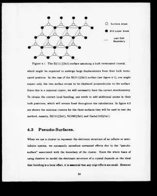
4.1 The S i ( ll l) ( 2 x l ) surface assuming a bulk terminated crystal. . . . 54

4.2 Minimal clusters for the S i( lll) ( 2 x l), Si(100)(2xl) and GaAs(llO)-( l x l ) surfaces... 55

4.3 Intermediate cluster for the S i(lll)(2 x l) surface... 60

4.4 Enlarged cluster for the S i( lll) ( 2 x l) surface... 60

5.1 Relationship o f the vectors used in equation 5.5... 67

6.1 The three possible sites for a single Pb atom on a Germanium sub­

strate with 3m symmetry... 80

6.2 The labelling system used by Pedersen (1987, 1988)... 81

6.3 The clusters used in the ETBM calculations for each of the three

sites T i , T* and H3. The arrows indicate the positive direction for

the in-plane displacements... 83

7.1 The sequence o f transitions observed on the SiC(lOO) surface by

Dayan. The temperature ‘T ’ is the transition temperature... 89

7.2 Dayan’s (1986) proposed model for the Si-(3x2) structure... 90

7.3 Dayan’s (1986) proposed model for the Si-(2xl) structure... 91

7.4 Surface unit cells for the C-(2xl) and Si-c(2x2) structures assuming

simple dimers... 92

7.5 Three models for the Si-(2xl) structure... 92

7.6 The (2x2) structures formed by the adatom models for the Si-(2xl)

structure if dimérisation occurs... 93

List o f Tables

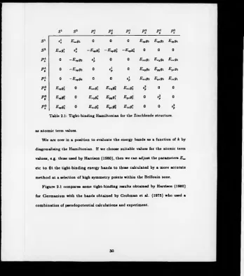
2.1 Tight-binding Hamiltonian for the Zincblende structure... 30

2.2 Expressions for LCAO and free-electron band energies (Froyen and

Harrison, 1979)... 34

2.3 Analytical expressions for the Universal Parameters (Froyen and

Harrison, 1979)... 34

2.4 Comparison o f d r2 scaling and a pseudopotential Hamiltonian (from

Smith 1986)... 39

3.1 Variations o f the S i(lll)(2 x l) Surface for Different Basis Sets. . . . 50

4.1 Comparison o f different treatments of the pseudo-surfaces of a min­

imal cluster with Chadi’s results for the S i( lll) ( 2 x l) surface. l6z’

is in the (1,1,1) direction... 58

4.2 Comparison o f different treatments o f the pseudo-surfaces of a min­

imal cluster with Chadi’s results for the Si(100)(2xl) surface. ‘ 6z’

is in the (1,0,0) direction and l6x' is in the (0,1,1) direction... 58

4.3 Comparison o f different treatments of the pseudo-surfaces of a min­

imal cluster with Chadi’s results for the G a A s(U 0 )(lx l) surface.

‘ 6z’ is in the (1,1,0) direction and ‘6x’ is in the (0,0,1) direction. . 59

4.4 Atomic displacements in angstroms for the S i(lll)(2 x l) surface. . 61

4.5 Atomic displacements in angstroms for the Si(100)(2xl) surface. . 61

4.6 Atomic displacements in angstroms for the G aAs(110)(lxl) surface.

The angle 0 is the tilt o f the planes containing the surface atoms

relative to the bulk... 62

5.1 Comparison of local minima using the self-consistent (SC), non-

self-consistent (NSC) and charge discrimination (6Qa) models for

the S i ( ll l) ( 2 x l ) surface. Also given is Pandey’s (1982) result. . . . 75

5.2 Comparison o f local minima using the self-consistent (SC),

non-self-consistent (NSC) and charge discrimination (6Q2) models for

the Si(100)(2xl) surface. The final column is the most stable o f the

symmetric dimers, and the energies are in eV ... 76

5.3 Comparison of local minima using the self-consistent (SC),

non-self-consistent (NSC) and charge discrimination (6Q2) models for

the G aA s(110)(lxl) surface. The single 0 is the tilt of the planes

containing the surface atoms relative to the bulk... 77

6.1 Displacements, in A, from bulk positions for the Germanium atoms

and a starting position for the Lead atom such that the Ge-Pb bond

length is 2.84 A. ‘h’ indicates in-plane displacements towards the

adatom, V indicates displacements normal to the surface (Peder­

sen, 1988)... 82

6.2 Atomic displacements:-A, atomic charges:-e and energie8:-eV for the

three clusters. The first figure in each box is the normal displace­

ment, the second is the displacement along the arrow directions o f

figure 6.3 in the surface plane and the third figure is the atomic

charge... 85

6.3 Comparison for the T 4 site o f the separations between various lay­

ers o f the P b -G e (lll) system. The first column gives the values

for bulk like starting position given before (with the Pb-Ge bond

length equal to 2.84

A),

measurements in

A

7.1 Dispacements in angstoms for the C -(2xl) and Si-c(2x2) structures,

charge in atomic units... 95

7.2 Displacements in angstroms for the three models for the Si-(2xl)

structure, charge in atomic units... 96

7.3 Normal and in-plane displacements for the two Si-(2x2) models,

charge in atomic units... 97

7.4 The total energies in eV for each of the (2x2) models considered. . 97

Acknowledgements.

I would like t o take this opportunity to thank some o f the many people who

have helped me reach the point where I am able to submit this

thesis:-• My parents and family for the support they have given to me over the years

o f my academic career;

• Dr B.W. Holland for his guidance, and for pointing me in the right direction

each time I forgot the aim o f the research;

• Dr V. Dwyer, Mr M. Kearney and Mr A. Wander for taking the time and

effort to explain things to me;

• Dr P.V. Smith for his critical reading o f this thesis;

• My colleagues at Warwick for their friendship;

• The Department of Physics for the provision of facilities and SERC for fi­

nancial support and the provision of computer resources;

• The staff o f Warwick University Computer Services, in particular Mr J. Hicks

for his assistance, and the staff of UMRCC and ULCC;

• Finally Ms Rona Tan for helping me type this thesis.

< _

Declaration.

This thesis (written in accordance with PHYS/PG3) contains an account of

my own research (except the work presented in section 5.2.1 and the self-consistent

result for the S i ( ll l) ( 2 x l ) surface in table 5.1, which was performed by Dr V.M.

Dwyer) carried out in the Department of Physics at the University of Warwick,

between October 1985 and August 1988, under the general supervision of Dr B.W.

Holland.

No part o f this work has been previously submitted to this o r any other aca­

demic institution for admission to a higher degree. Some parts o f it have already

been published, and are as follows:

• Empirical Tight-Binding Cluster Method for Semiconductor Surface Struc­

tures,

J.N. Carter, V.M. Dwyer and B.W. Holland.

Surface Science L723, 1987.

• Charge Self-Consistent Empirical Tight-Binding Cluster Method for Semi­

conductor Surface Structures,

V.M. Dwyer, J.N. Carter and B.W. Holland.

Proceedings of the Second International Conference on the Structure of Sur­

faces, Springer Series in Surface Sciences, H , 320, 1988. Editors J.F. van

der Veen and M.A. Van Hove.

• Structure o f the a phase o f G e(lll)>/3x>/3-Pb,

J.N. Carter, V.M. Dwyer and B.W. Holland.

Solid State Communications, fiZ, 643, 1988.

It U hoped to publish the work in chapter 7 on the (100) surface o f Cubic Silicon

Carbide in the near future.

Ty.hl

J.N. Carter

A bstract.

In this thesis a cluster method for evaluating the structure of semiconductor

surfaces is formulated. Chadi’s total energy algorithm is used to express the total

energy o f a cluster in terms o f a sum o f one-electron energies and a residual energy

term. T h e one-electron energies are calculated within Harrison’s Tight-Binding

Approximation, using his empirical interatomic matrix elements. The residual

energy, being the difference between the ion-ion and electron-electron interaction

energies, is treated as a bond stretching energy summed over all bonds in the

cluster. The energy o f a bond is evaluated by comparison with the change in energy

as a function of bond length as determined by a quantum chemistry calculation.

A cluster includes all the atoms that are expected to be displaced from their bulk

positions and enough other atoms such that displaced atom s have the correct local

bonding. The edge o f the cluster is saturated with Hydrogen atoms. A form of

self-consistency is included by relating the distribution o f charge to changes in the

atomic term values and iterating the process until self-consistency is achieved. The

model is tested on the S i( lll) ( 2 x l), Si(100)(2xl) and G aA s(110)(lxl) surfaces,

and then used for calculations on the G e (l ll ) and /?-SiC(100) surfaces.

Abbreviations.

AES Auger Electron Spectroscopy

BCC Body Centred Cubic

CVD Chemical Vapour Deposition

ETBM Empirical Tight-Binding Method

FCC Face Centred Cubic

LCAO Linear Combination o f Atomic Orbitals

LEED Low Energy Electron Diffraction

MBE Molecular Beam Epitaxy

NSC Non- Self- Consistent

SC Self-Consistent

SERC Science and Engineering Research Council

SEXAFS Surface Extended X-ray Absorption Fine Structure

SXD Surface X-ray Diffraction

UHV Ultra-High Vacuum

ULCC University o f London Computer Centre

UMRCC University of Manchester Regional Computer Centre

“There is no such thing as a problem without a gift for you in its hands.

You seek problems because you need their gifts.”

— Richard Bach, Illusions.

Chapter 1

Motivation and Preview.

“Begin at the beginning” , the king said, gravely, “and, go on till you

come to the end: then stop.”

— Lewis Carroll, Alice in Wonderland.

1.1

M otiva tion .

The advances that have been made in the last decade in the fabrication of solid-

state devices have been dramatic, with the scale o f the devices becoming such

that their behaviour is beginning to depend on surface and interface effects. Also

there has been the development of Molecular Beam Epitaxy (MBE) to the point

where devices o f one or two monolayers can b e put down (Sano et al., 1984),

in such devices it is important to know how th e surface grows. To understand

both surface and interface effects it is necessary to know the electronic structure

involved, this is directly dependent on the atom ic structure found (which may be

very different from that to be found in the bulk crystal).

The experimental study of surfaces has developed mainly in the last twenty-

five years with the development of ultrarhigh vacuum technology (UHV), there

now exists a wide range o f surface sensitive techniques available including: Low

Energy Electron Diffraction (LEED), Auger Electron Spectroscopy (AES) and

Surface Extended X-ray Absorption Fine Structure (SEXAFS). For an extensive

guide to the properties of surfaces and the techniques for studying them one should

consult books by Zangwill (1988), Woodruff and Delchar (1986).

From a theoretical point of view, without reference to experimental data, about

the only option available to determine surface structure is some form o f total energy

minimisation. Attempts to do this with respect t o the structural parameters of the

surface have generally followed one of two approaches. The “Solid-state” approach

(Chadi, 1978; Pandey, 1982), in which Bloch’s theorem plays a central role, and

which cannot treat non-periodic defects; or the “Chemical” approach (Swarts,

1981; Barone, 1985) in which the surface is represented by a small atomic cluster

on which the sophisticated methods of quantum chemistry are used. Both methods

obtain results which are comparable to experiment.

The principle difficulty with the quantum chemistry methods is that they can

only treat small clusters of atoms, because o f the excessive demands made on

computer time. The same problem exists for the solid-state approach when first-

principle self-consistent methods are used (Pandey, 1982). Chadi (1978) has shown

that valuable results can be obtained when using an empirical tight-binding model

within the solid-state approach. The aim of the work presented in this thesis is to

develop a model similar to that proposed by Chadi and apply it to atomic clusters,

there by obtaining a significant computational advantage over the solid-state and

chemical approaches.

1.2

Preview’ .

In chapters 2-5 the aim is to develop a tight-binding model that can be applied

to atomic clusters to give reasonable predictions o f the atomic structure of semi­

conductor surfaces. To achieve this I started with Harrison’s (1980) tight-binding

model and used this within Chadi’s (1978) total energy algorithm. This then allows

one to develop a consistent methodology for the construction and enlargement of

atomic clusters to mimic the behaviour of the crystal surface. In this thesis I have

outlined the necessary theory developed by other authors and then applied this to

the clusters. Chapters 6 and 7 cover some examples o f the methods application to

semiconductor surfaces. The last chapter is a review and also looks at some points

that could be examined within the model.

1.2.1 Chapter 2.

In this chapter the aim is to examine the ground on which Harrison’s (1980)

tight-binding model is built. This starts by outlining how to construct the one-

electron wave function o f a polyatomic system. This leads directly to the cal­

culation of the band-structure of a periodic crystal. At this point some of the

ideas o f tight-binding models are introduced. T h e one-electron wave function is

expressed as a linear combination of atomic orbitals (LCAO). When calculating

the band-structure, the overlap between atomic orbitals on different atoms is ig­

nored. Only interactions between atomic orbitals on nearest-neighbour atoms are

included. The LCAO band-structure is “fitted” to the band-structure determined

by more accurate methods to determine the matrix elements which represent the

nearest-neighbour interactions. Next is introduced Harrison’s discovery that these

parameters scale from material to material in a predictable way. The chapter con­

cludes with a brief examination o f the work that has been done to support the

assumptions used within the model.

1.2.2

Chapter 3.

In this chapter the intention is to develop a particular model for the total energy o f

a cluster of atoms. The aim o f the work that follows in later chapters is to find the

minimum o f this total energy with respect t o “some” structural parameters that

describe the cluster. We use a total energy algorithm introduced by Chadi (1978),

in which the total energy is split into two terms; a sum of one-electron energies

and a residual energy term. The residual energy accounts for the double counting

o f some energy terms in the one-electron energies and those terms not included in

it. The residual energy is expressed as a b on d stretching energy. The rest o f the

chapter considers how this algorithm is to be applied to clusters, using Harrison’s

tight-binding model for the one-electron energies and a quantum chemistry package

to help calculate the bond stretching energy term.

1.2.3 Chapter 4.

Having a way o f calculating the total energy o f a given cluster, attention is now

turned to how to construct a cluster so that it mimics the behaviour of an infinite

periodic system. Fortunately it appears that bonding within a covalent system is

a highly localised effect, and as such, a small cluster has a very similar electronic

structure to an infinite surface. The work starts by examining the cluster needed

to represent a single unit cell on the surface. Th ere then follows a consideration of

how to treat the unwanted surfaces (pseudo-surfaces) which exist only because we

are using a cluster and not a semi-infinite solid. T h e chapter concludes by looking

at how to systematically extend the cluster. T h e accuracy of the predictions are

then compared to the results obtained for different cluster sizes and for different

surfaces with those o f other authors.

1.2.4 Chapter 5.

In developing the model so far, one important point has been ignored. It is that the

energy levels used to calculate the sum of one-electron energies are dependent on

the charge distribution in the cluster, and the charge distribution is dependent on

which one-electron energy levels are occupied. It is clearly desirable to calculate the

one-electron energies in a self-consistent manner. The tight-binding model being

adjusted in an iterative manner until self-consistency is achieved. To account for

the self-consistency, the atomic term values used in the one-electron Hamiltonian

are changed at each iteration in the way prescribed by Harrison (1985). This

involves the charge of the atom under consideration and the Coulomb potential due

to the infinite periodic array of charge produced on the surface. Also considered is

an ad hoc method which discriminates against a build up of charge on a particular

atom, which is the main effect seen in the non-self-consistent calculations. Both

methods are compared against results produced by other means.

1.2.5 C h a p te r 6.

This work represents the first attempt to use the method in a regime where there

are no previous calculations to compare with. It has been shown by a number

o f researchers, that for low coverages o f Lead on the Germanium (111) surface

there exist two differing phases, each with a \/3x\/3R30o reconstruction pattern,

but at different coverages. It has been agreed that the first of these phases has

a single Lead atom per unit cell and that it appears to occupy a high symmetry

site. The aim o f the work was to determine which o f the three possible sites had

the lowest energy and the positions o f the atoms within the unit cell. The results

are compared with the predictions obtained from the analysis o f Surface X-ray

Diffraction work.

1.2.6 Chapter 7.

This chapter deals with a surface for which there is much greater uncertainty and

less experimental work. The surface in question is the (100) surface o f Cubic

Silicon Carbide. Starting from the as received samples with a surface coating of

Silicon Dioxide, a sequence o f different LEED patterns are seen as the surface is

annealed. The aim of the work was to examine some o f the possible structural

models for the surface and to predict which are possible models based on the

energy o f each o f the systems and the charge distributions found in the minimum

energy configurations.

1 .2 .7 C h a p ter 8.

The thesis finishes with a review o f the conclusions reached and the results ob­

tained. The chapter also contains a consideration o f problems to which the model

might be applied and possible variations to its formulation that might be consid­

ered within the model.

Chapter 2

Tight-Binding M odel.

“To accept the arguments o f science, is to voluntarily accept other

peoples errors.”

— Alexander Solzhenitsyn, Cancer Ward.

2 .1

H is t o r ic a l D e v e l o p m e n t .

The forerunner of the Empirical Tight-Binding Method (ETBM) known as the

Linear Combination of Atomic Orbitals (LCAO) method first saw the light of day

in a paper by Bloch (1928) in which he proposed a method to solve the problem

o f a set of N atoms at the vertices o f an N-sided regular polygon. The basic idea

was to use a linear combination o f the atomic orbitals of the atoms in the ring to

approximate the complete wave function. For a ring of ‘AT’ atoms with separation

‘o ’ it can be shown that

® (x) = Uk(x)exp(i2irsx/Na) (2.1)

(Kittel, 1976, pl90) where

• € { 0 . . . N - 1), (2.2)

provided that t/fc(x) = U k(x+ a). Such a function is given by the sum o f the atomic

orbitals of one type o f all the atom s in the ring. If we take a linear combination

o f all the orbitals on all the atoms, we get

* (* ) = £ * «(*) e*p(>2

itax/Na).

From a ring o f identical atoms it is easy to generalise to an infinite chain of atoms,

and hence to 3D crystals. This work underlies much o f the work on the quantum

theory o f solids.

While the basic idea is easily carried over to solids, there are however a large

number o f very difficult integrals to be calculated which made the method nearly

impossible to do with complete rigour. Given these points Slater and Koster (1954)

proposed that the LCAO method should be used “not as a primary method o f ac­

curate calculation, but rather as an interpolation method” . Their principle method

o f attack was to retain only those terms (matrix elements) which were required to

give qualitative correctness to the method and to treat them as adjustable parame­

ters which are fitted to the results o f more accurate calculations at high symmetry

points of the Brillouin zone.

With the advent of new methods and more powerful computers the need for

an interpolation method diminished.

In recent years the method has been turned from an interpolation scheme for

the band structure of crystalline solids, to an extrapolation scheme for amorphous

solids and perturbed crystals, e.g. surfaces.

2.2

Linear C o m b in a tio n s o f A to m ic Orbitals.

In this chapter the aim is to outline the ideas behind the tight-binding model. We

start here with the ideas that underlie the LCAO method.

The prime assumption that we use is that the one-electron wave function o f a

polyatomic system can be written as a sum o f atomic basis functions

!»..(«•) > = E K i \ M T - * ) ) > • (2-4)

aj

where

• |¥„(r) > is the one-electron wave function

• |^a(** — R j) > is the atomic orbital |^a(r) > on the jth atom

the sum being over all orbitals and atoms.

If we substitute equation 2.4 into the time-independent Schrodinger equation

we obtain

£

F ^ H ^ J r

Rj)

- R , ) > ,

aj a j

where H is the one-electron Hamiltonian and E v is an eigenvalue. If we now

pre-multiply by < <t>p(r — we obtain a series of simultaneous equations

£ F * , - * . ) . (2 6)

aj a j

where

H „ A R . - R j) = < M r - R.)\H\Mr - R j) > (2.7)

and

Sß+(Ri - R,)

M r -

R,)

Equation 2.6 may be written in the form o f a matrix equation

H F* = E 'S F *, (2.9)

hence we need to solve

det(H - E "S ) = 0 (2.10)

(we may then solve for F v also).

For a crystalline solid, we may according to Bloch’s theorem, write F ^ in the

following form

F ;, = c ;( k ) 'x p ( i k J t ,) (2.11)

(j/ = n,k , where n numbers the solutions for a given k), R} being the bravais

lattice sites. Equation 2.6 can now be written in the following form

£ { * . . . ' < * ) - - 0 (2.12)

with

H ^ ( k ) - N - ' Y . ^ M ' k - R , ) H . ^ R , ) (2.13)

and

S__•(*) = N - ' Y . ' * v ( ‘ k R , ) S . ^ R , ) , (2.14)

N being the number o f lattice sites in the crystal. Equation 2.10 is now written as

det(H (k) - En(k)S (k)) = 0. (2.15)

Solving equation 2.15 yields the energy bands En(k) o f the crystal.

From equation 2.15 it is possible to proceed in a variety o f different ways

depending on what prescription one uses to evaluate equations 2.7 and 2.8. One

could proceed directly and evaluate each o f the terms Ha,a' and Sa,a<, this however

becomes difficult due to the number of multicentral integrals. An alternative

approach is that of the Extended Huckel Method in which it is assumed that Haa'

is proportional to Sa,a' (<* and a ' are not on the same atom).

The way we proceed is that set out by Slater and Koster (1954) in which they

treat the Hamiltonian elements H a,a' as parameters which are fitted to accurate

calculations at high symmetry points of the Brillouin zone.

2.3

B a n d S tru ctu re Calculations.

Following the work of Slater and Koster (1954) a number o f groups used the

LCAO method as an interpolation scheme. In particular I wish to follow the work

published in a paper by Chadi and Cohen (1975) which contains many o f the

simplifications that are used later by Harrison (1980).

Let us consider the case o f diamond or zincblende crystals. Within each pri-

mative cell there are two inequivalent tetrahedrally coordinated atoms, which can

be labelled ‘ type 1’ or ‘type 2*. If we have two sets o f tight-binding basis functions

|^i(r - R j) > and |0„(r - R3) > (R j defines a bravais lattice centred on the atom)

then from equations 2.4 and 2.11 we may construct the following Bloch functions,

|*i(*,r) > = A T 1 2 > x p (;*.*,)| *i(r - « , ) > (2.16) i

■ |*i(*,r) > = A T 1 5>xp(.ir..R,)|*i(r - * , ) > . (2.17) >

An assumption that can be placed on the one-electron wave functions > is

that they are orthonormal (this is done to simplify the computation involved), i.e.

< * i(* ,r)| * i.(* ,r ) > =

6

from equations 2.16 and 2.17 we get,

A r 25 > x p (-i* .ft,)e x p (i* -R „) < *(>• - R l W A ' - * » ) > = ^ v*. (2.19)

which can only be true if

< 4>i(r - Ri)\</i.{r - J U > = S w (2.20)

If we now assume that the orbitals \Pa > are in fact the atomic orbitals at each

site, then equation 2.20 becomes

<

SaijAi

(this assumption will be considered in section 2.5.4). Hence equation 2.15 reduces

to

d e t(tf(* ) - £ . ( * ) ) = 0. (2.22)

The basic problem is to evaluate the matrix elements between the var­

ious atomic orbitals. Following Chadi (1977), let us assume that for diamond and

zincblende crystals only the outermost 15 > and three |P > orbitals are important

at each site. Then the Hamiltonian can be written as an 8x8 matrix.

Let us consider now how we build the Hamiltonian by looking in detail at the

matrix element between the atomic orbitals |5‘ > and |52 > , from equation 2.13.

« » . * ( * ) - J V - '£ e x p ( - i * R ,) N - ' J > x p ( i* .f i,) < S ‘ (r - *,)|«|S*(r - R .) > ,

7 •

(2.23)

now since the two bravais lattices defined on each o f the two atom sites are sep­

arated by d1, where d1 is the vector joining the atoms in the unit cell. If we now

relate the two bravais lattices to a single lattice by

Ri = R, + < f (2.24)

and make the following substitution (dropping the reference to the atoms, Harri­

son, 1980, p77)

E .. = < S ‘ (r - H,)|W|SJ(r - f t ) > (2.25)

then the Hamiltonian element becomes

Hs>s*{k) = J > x p <p

If we now restrict the sum over tf to nearest-neighbours (this being the Tight-

Binding Approximation (T B A )), then

HSxs»(k) = gi( k )E „ (2.26)

with

and

ffi(k) = exp(ik.di) + exp (ik.dj) + exp (ik.d3) + exp(ifc.d4) (2.27)

d, = ( l , l , l ) a / 4

¿2 = (1»1»I)<*/4

d3 = ( I , l , I ) a / 4

d4 = ( I , I ,l ) a /4

(2.28)

‘a’ is the lattice constant.

O ne can carry out similar calculations for each o f the Hamiltonian elements,

when we do this we find we need the following relationships

92(k) = exp(ik.di) + exp(ik.d2) - exp(ik.d3) - exp(ik.d4)

93(k) = exp(tk.di) - exp(ik.d2) + exp(ik.d3) - exp(*fc.d4) (2.29)

g4(k) = exp(ik.di) - exp(ik.th) - exp(ik.d3) + exp(tfc.d4)

Then using the fact that the Hamiltonian Matrix is hermitian we can write down

the matrix given in table 2.1. The elements down the leading diagonal are known

s l s 7 P i P i P i P i P i P I

s l l\ E—9l 0 0 0 E.Pg2 E^gz E.pgi

s 2 E..91 4 - E v gZ - E . r9l —E,vg\ 0 0 0

p ; 0 - E Mpg2 4 0 0 E xxgi Exyg* Extgz

p i 0 - E v g3 0 4 0 E.,9* E„ 9i Eyxgz

P\ 0 - E tpgt 0 0

4 Exxgz Eyxg2 Exxgi

p i E.r9'2 0 Exxg\ ExV9a E..9Î 4 0 0

p i E>p9i 0 E;9 \ Er.9l Eyxg2 0

4 0

p ; E.r9l 0 e..9 ; Eyxg2 E ..9i 0 0 ₄

Table 2.1: Tight-binding Hamiltonian for the Zincblende structure.

as atom ic term values.

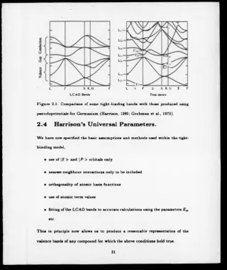
W e are now in a position to evaluate the energy bands as a function of k by

diagonalising the Hamiltonian. If we choose suitable values for the atomic term

values, e.g. those used by Harrison (1980), then we can adjust the parameters £ „

etc t o fit the tight-binding energy bands to those calculated by a more accurate

m ethod at a selection o f high symmetry points within the Brillouin zone.

Figure 2.1 compares some tight-binding results obtained by Harrison (1980)

for Germanium with the bands obtained by Grobman et al. (1975) who used a

combination of pseudopotential calculations and experiment.

Li,—

' l r x k.u r l a r a xk. u e

L C A O Bands True bands

Figure 2.1: Comparison of some tight-binding bands with those produced using

pseudopotentiais for Germanium (Harrison, 1980; Grobman et al., 1975).

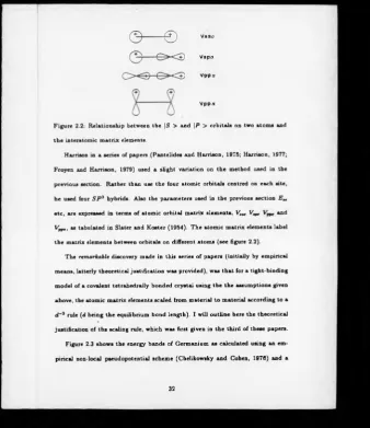
2 .4

H arrison ’s U niversal P aram eters.

W e have now specified the basic assumptions and methods used within the tight-

binding model,

• use of | S > and | P > orbitals only

• nearest-neighbour interactions only to be included

• orthogonality o f atomic basis functions

• use of atomic term values

• fitting of the LCAO bands to accurate calculations using the parameters E „

etc.

T h is in principle now allows us to produce a reasonable representation of the

valence bands o f any compound for which the above conditions hold true.

© — ©

Q c x g

V s s a

V s p a

O < D C X S v p p°

Vpp«

Figure 2.2: Relationship between the |S > and |P > orbitals on two atoms and

the interatomic matrix elements.

Harrison in a series of papers (Pantelides and Harrison, 1975; Harrison, 1977;

Froyen and Harrison, 1979) used a slight variation on the method used in the

previous section. Rather than use the four atomic orbitals centred on each site,

he used four S P3 hybrids. Also the parameters used in the previous section E „ etc, are expressed in terms of atomic orbital matrix elements, V,.a Vtpa and

Vpp*, as tabulated in Slater and Koster (1954). The atomic matrix elements label

the matrix elements between orbitals on different atoms (see figure 2.2).

The remarkable discovery made in this series of papers (initially by empirical

means, latterly theoretical justification was provided), was that for a tight-binding

model of a covalent tetrahedrally bonded crystal using the the assumptions given

above, the atomic matrix elements scaled from material to material according to a

d r2 rule (d being the equilibrium bond length). I will outline here the theoretical justification of ths scaling rule, which was first given in the third of these papers.

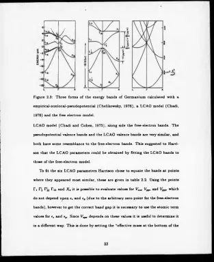
Figure 2.3 shows the energy bands of Germanium as calculated using am em­

pirical non-local pseudopotential scheme (Chelikowsky and Cohen, 1976) and a

S - !

Figure 2.3: Three forms o f the energy bands of Germanium calculated with a

empirical-nonlocal-pseudopotential (Chelikowsky, 1976), a LCAO model (Chadi,

1976) and the free electron model.

LCAO model (Chadi and Cohen, 1975), along side the free-electron bands. The

pseudopotential valence bands and the LCAO valence bands are very similar, and

both have some resemblance to the free-electron bands. This suggested to Harri­

son that the LCAO parameters could be obtained by fitting the LCAO bands to

those o f the free-electron model.

To fit the six LCAO parameters Harrison chose to equate the bands at points

where they appeared most similar, these are given in table 2.2. Using the points

r i r 2 Tjs Tl5 and X* it is possible to evaluate values for Vtsa V^, and which

do not depend upon e, and ep (due to the arbitrary zero point for the free-electron

bands), however to get the correct band gap it is necessary to use the atomic term

values for e, and tv. Since V ^ depends on these values it is useful to determine it

in a different way. This is done by setting the “effective mass at the bottom of the

Point LCAO Free-electron

r . e* + 4V”W 0

n «. - 4V.„

rw

Tl5 *, + + JV^,

Jf.

■ M W -fK S T

x 4 H - t V m + iV m

-Table 2.2: Expressions for LCAO and free-electron band energies (Froyen and

Harrison, 1979).

v . „

V r

-Table 2.3: Analytical expressions for the Universal Parameters (Froyen and Har­

rison, 1979).

‘ S’ band equal to the free-electron mass” (for the details see Froyen and Harrison,

1979).The values obtained by Froyen and Harrison are given in table 2.3. Using

exactly this approach it was possible to evaluate appropriate parameters for other

structures (simple cubic, FCC, BCC).

It is these “universal parameters” that we will be using in later calculations.

2.5

C ritique o f H arrison ’ s T igh t-B in d in g M odel.

In this section I wish to examine in greater detail some o f the work that supports

the main assumptions within tight-binding models in general and Harrison’s model

in particular, the assumptions being: the need for |5 > and |P > orbitals only,

nearest-neighbour interactions only, the scaling rule for the universal parameters

and the orthogonality o f the basis set.

For a more general critique o f tight-binding methods for semi-conductors one

should read Pantelides and Pollmann (1979).

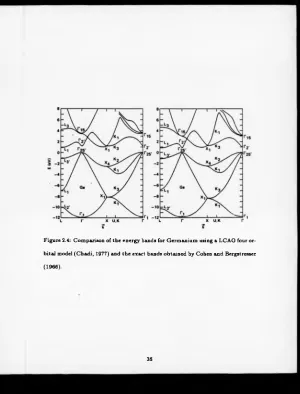
2.5.1 Size o f Basis Set.

T o examine the question as to how large the basis set needs to be it is useful not

to work within a tight-binding model, but to use a more accurate technique. This

was done by Chadi (1977) when he used an empirical pseudopotential Hamiltonian

to predict the band-structure o f Silicon, Germanium and Gallium Arsenide.

He considered two cases, the first involved four basis functions (one |5 > and

three |P > ) per site, the second had five additional |d > orbitals and one “/-like”

orbital. In figure 2.4 are the results for Germanium using four basis functions

compared to the exact results obtained by Cohen and Bergstresser (1966).

Chadi made the following conclusion:

“We have shown that a simple basis set consisting o f |5 > and |P >

orbitals can give an accurate description of the valence and conduc­

tion band-structures o f diamond and zincblende semiconductors. For

accurate energy bands and wave functions we find a ten state per atom

Figure 2.4: Comparison of the energy bands for Germanium using a LCAO four or­

bital model (Chadi, 1977) and the exact bands obtained by Cohen and Bergstresser

(1966).

basis that includes |d > orbitals to be sufficient for the valence and the

first few conduction bands.”

Since we will be only interested in the valence bands, the |S > and |P > basis

set should be adequate for our purposes.

2.5.2

Nearest-Neighbour Interactions.

While it is true that the eigenstates o f a covalently bonded crystal are not confined

to a particular region, it is found however that the amplitude o f the wave function

is o f significance only in a fairly small region. Therefore one only needs to include

interactions within a limited area.

The question as to which interactions should be included is most often decided

by the accuracy that is required for the valence bands, it is unusual for more than

second nearest-neighbour interactions to be included (see Chadi and Cohen, 1975).

In their paper Pantelides and Pollmann (1979) offer the following exposition of

the Tight-Binding Approximation. Consider a simple linear chain of atoms with

atomic spacing ‘a’ , then equation 2.13 may be written as

Haa'(k) = Vi cos(fca) + 53 V* cos(nfca) (2.30)

where

Vn = Haa‘ (R j) j = nth neighbour shell (2.31)

If we define

(2.32)

then we may write

Haa. = \(k)VlCos(ka) (2.33)

if we compare this to the tight-binding equivalent (c.f. equation 2.26)

Haa> = Vco*(ka) (2.34)

one can see that the tight-binding model replaces \(k)Vi with its average over the

Brillouin zone. This argument can clearly be extended from infinite chains to 3D

crystals.

2.5.3 Scaling R u le for the Universal Parameters.

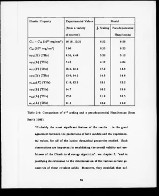
Harrison’s d~2 scaling rule was established by examining how the interatomic ma­ trix elements scaled from material to material. As pointed out by Smith (1986),

“the real question . .. is whether this d~2 ansatz correctly describes the way in which the LCAO interatomic matrix elements o f a given covalent solid vary with

interatomic spacing.”

In a series of papers (Smith and McMahon, 1983; Robertson, 1983; Smith,

1985, 1986) the tight-binding parameters were fitted to pressure dependent pseu­

dopotential band-structures. Then the variation of the parameters was compared

to those predicted by the d~2 scaling rule, it transpires that the d~2 scaling rule always under-estimates the variations. Smith (1985, 1986) also checked some of

the predictions for bulk properties made by Chadi ( 1978) (this is of much greater

importance from the position of the work presented in this thesis, because in later

chapters we will be using what is essentially Chadi’s total energy model). In table

2.4 are the values produced by Smith (1986) for the elastic constants and of the T

and X point phonon frequencies of Silicon.

Quoting from Smith’s (1986) results:

Elastic Property Experimental Values

(from a variety

o f sources)

Model

Jr Scaling Pseudopotential

Hamiltonian

C „ - C ,i (1011 erg/cm 3) 10.18, 10.21 8.52 8.56

Cu (1011 erg/cm3) 7.96 8.25 8.22

(THz) 4.35, 4.49 5.20 5.12

^ta(L ) (THz) 3.43 4.12 4.04

<*ro(r) (THz) 15.5, 15.3 17.3 14.8

w ro (X ) (THz) 13.9, 14.2 14.9 14.8

*lao( X ) (THz) 11.9, 12.3 13.1 12.2

uto(L ) (THz) 14.7 16.2 15.8

ulo(L ) (THz) 12.6 11.6 10.5

u<la(L ) (THz) 11.4 13.2 11.0

Table 2.4: Comparison o f d 2 scaling and a pseudopotential Hamiltonian (from

Smith 1986).

“Probably the most significant feature o f the results . . . is the good

agreement between the predictions of both models and the experimen­

tal values, for all o f the lattice dynamical properties studied. Such

observations are important in establishing the overall validity and use­

fulness of the Chadi total energy algorithm” , see chapter 3, “and in

justifying its extension to the determination o f the various surface ge­

ometries of these covalent solids. Moreover, they establish that

ficient compensation always occurs within the Chadi total energy al-

gorithm between the band-structure contribution, Ebs. and the short

range force term, U, to result in values which are relatively insensitive

to the choice o f spatial model.”

What would be particularly useful would be the repetition o f Chadi’s surface

calculations but using a Hamiltonian fitted to the pressure dependent pseudopo­

tential band structure. However at this time such calculations have not been

performed.

2.5.4

O rthogonality o f the Basis Set.

When we developed the tight-binding model of the band-structure in section 2.3, it

was necessary to assume that all the atomic orbitals were orthonormal (equation

2.21), this assumption is clearly untrue. The point was resolved in a paper by

Lôwdin (1950). I shall present here the case for molecular orbitals which will be

needed in later chapters. For the Bloch orbitals that were used in section 2.3

arguments very similar to those given below apply to give the same final result,

however I will not deal with the details here.

For molecular orbitals we have (equation 2.9)

H F " = E * S F (2.35)

and from equations 2.4, 2.8 and 2.18 we get

F ^ S F * = 1 (2.36)

(where F**' is the complex conjugate o f F").

L e t u s d e f i n e

F v = 5 - 1/aC*' (2.37)

(where 5 -1/a is some matrix such that S“ 1/a5 _1/a = 5 -1 ), substituting this into

equation 2.9, we have

H'CT = C E T , (2.38)

with

H' = S - '^ H S - 1' 2. (2.39)

We therefore need to solve

d et(tf' - E ) = 0 (2.40)

which has the same form as equation 2.22.

Quoting from Lowdin’s paper:

“The problem of solving the secular equations including the overlap

integrals SM„ can be reduced to the same form as it has in the simplified

theory ( S neglected) if the matrix H is replaced with the matrix H ’ .n

Since the Hamiltonian matrix elements are determined empirically they can be

considered to be the elements o f H' rather than H .

What we have done here is to take the original localised basis set and replace

it with a orthogonal basis set which is a linear combination o f the original basis

set . In doing this the new basis set tends to be less localised than the orbitals

with which we started.

Chapter 3

Evaluation of the Total Energy.

“In these days, a man who says a thing cannot be done is quite apt to

be interrupted by some idiot doing it.”

— Elbert Hubbard.

3.1

In trod u ction .

The aim o f the work is to minimise the total energy with respect to the structural

parameters of a particular cluster of atoms, which are intended to approximate to

a crystal surface. For a specific cluster the total energy is calculated using a sum

of one-electron energies and a parameterized form for the residual energy.

The total energy o f an electron-ion system can be written as the sum o f four

terms:

Ejt = Eke + Eie + Eee + Ea, (3.1)

• Eke the electron kinetic energy term,

• E ie is the ion-electron interaction energy,

• Eee is the electron-electron interaction energy,

• Ea is the ion-ion interaction energy.

Let us first consider the information contained within a sum o f one-electron

energies. In particular it can be shown that within the Hartree-Fock method (see

appendix A ) that;

+ 4 . + 2 4 . (3.2)

(where S i signifies the sum over occupied one-electron states of the occupancy

o f the state multiplied by its energy). If we define

U = Ea - E „ , (3.3)

then the total energy can be written in the form,

ET = ’£ lt + U. (3.4)

The S i fi term will be calculated within Harrison’s (1980) tight-binding model.

Following Chadi (1978) we note: “that for ions that are separated by a dis­

tance much larger than the Thomas-Fermi screening length the combined ion-

plus-screening-electron system is nearly neutral and U is close to zero. One would

therefore expect that to a good approximation this term can be described by a

short-range-force-constant model.”

Like Chadi we will treat U as a bond stretching energy, which is expressed as

a polynomial expanded about the equilibrium bond length,

u = (*■»)

•<> »

where

• dij is the distance between atoms li\ and‘j ’ ,

• djy is the equilibrium bond length between atoms ‘i’ and ‘j\

. «> = ( * , - < ) / < .

3.2

Sum o f O n e-electron Energies.

The basic assumptions which underlie Harrison’s tight-binding model (nearest-

neighbour interactions, |S > and | P > orbitals only and a l / d 2 dependence of

the matrix elements) remain unchanged when we move from a bulk calculation to

a surface. What one might expect to change are the parameters VtMr,

and V ^ . The assumption that is normally made is that these parameters are

equally suitable for calculations on the surface or in the bulk. The justification

for this comes from the use of the LCAO method to calculate surface electronic

properties, when exactly this assumption is utilized (Pantelides, 1977), and the

very good agreement with self-consistent pseudo-potential calculations obtained is

used to justify the assumption.

Let us now consider how to construct the Hamiltonian using Harrison’s pre­

scription, which will give the required one-electron energies, for a cluster. In the

case of a tetrahedrally bonded covalent solid, each atom in the equilibrium bulk

state has four bonds, which are equally spaced about the atom. If we take a linear

combination o f the outermost |5 > and three |P > orbitals on a particular atom,

we can construct four orthonormal wave functions which have their probability

d i s t r i b u t i o n s p o i n t i n g in t h e d i r e c t i o n s o f t h e b o n d s , i .e .

|hi > = ^{|S > + |P* > + |P* > + |Px > } with direction [11/],

|h2 > = ^{|S > + |P* > ~\Py > —\P* > } with direction [ i l l ] , (3.6)

\h3 > = ^{|5 > -| P , > + |P, > -|P , > } with direction [ I I I ] ,

|h4 > = ^{|5 > -|Pr > —|Pf > +|P, > } with direction [ I I I ] .

We are justified in doing this, since taking linear combinations of atomic orbitals

is equivalent to doing a unitary transformation on the Hamiltonian matrix. It is

easy to show that these hybrids are orthonormal, < h,\hj > = 6tJ (since the |S >

and |P > orbitals on a single atom are orthonormal).

Any rigid rotation of this set of wave functions will produce another orthonor­

mal set, in particular the set with hybrids pointed in the opposite direction to those

given above. For those atomic elements which require the use o f the outermost

|5 > orbital only, then there is only one hybrid which takes the form,

|h > = 15 > . (3.7)

If we have a cluster o f atoms { t } at positions {?*<} and each atom within the

cluster has hybrids \h'a > , then we need to evaluate the Hamiltonian matrix el­

ements H dfij = < h*a\H\hj0 > . The matrix elements are split into three groups depending on the relationship o f the atoms ‘t’ and lj ' .

If we write the hybrids in the form,

(3-8)

where a'al/ are the coefficients, in equations 3.6 and 3.7, related to atomic orbitals

\4>'u >. When * = j , i.e. hybrids on the same atom,

Hai# =

= (3-9)

*<

since < 4>lv\H\4>\ > = . where e„ is an atomic term value,

^ Haifii = ^ aL ° L ty (3.10)

1/

When and ‘j ’ are nearest neighbour atoms, i.e. they are bonded covalently

to each other, then we make use of the Slater-Koster (1954) interatomic matrix

elements,

HaiJIj ~

K

= (3 1 1 )

•<

For |5 > and |P > orbitals the Slater-Koster interatomic matrix elements are in

terms o f the parameters that Harrison used,

• Es,s = v „ ,

• Es.Pm = — E p . , S — IVtjKr,

• Es.p, = - E p t,s = mVtpa,

• Es.p, = —Ept.s = nV,,*,,

• Ep.,p. = + (1 - P ) V „ ,

• E r,.r, = maVpfw + (1 - m * )V „ ,

• E ,„ r , = + (1 - nJ)V V .

•

E Pm_pt = E Pt,p.

V ^ ),

• Ep.'P. = Ep.,Pm = In iY ^ - V „ ) ,

• = Ep„pt = mniVpp,, - Vpp*),

l, m, n are the direction cosines of the bond between the atoms ‘t’ and ‘j\

In all other csises the Hamiltonian matrix element is zero, because we assume

that we need include only interactions between nearest-neighbour atoms.

Having constructed the Hamiltonian one can evaluate the ordered set o f eigen­

values e,, with t\ being the eigenvalue o f lowest value. If the cluster has M valence

electrons, then the sum of one-electron energies over occupied states is given by

putting two electrons into each eigenstate starting with the one with lowest en­

ergy (¿i) and proceeding up the list until all of the electrons have been placed in

an eigenstate. If we have an odd number of electrons then the highest occupied

eigenstate will only have one electron in it. The sum o f the one-electron energies

is given by

where [P] is the largest integer P1 < P.

3.3

B o n d Stretching Energy.

In Chadi’s (1978) original paper he used two conditions on the total energy to

fix the coefficients U\ and U2 in equation 3.5. The conditions were that at the equilibrium bond length the total energy of the bulk crystal was at a minimum,

[M/2|

= 2 ^ 2 €i + (M - 2[M /2])c[a#/2)+i, (3.12)

dEp I

= 0 (3.13)

(V

(B being the bulk modulus). Rather than following Chadi’s approach of using

bulk crystal properties to evaluate the various coefficients Un in equation 3.5, we

proceeded to evaluate U(d) for a small molecule by using a quantum chemistry

package (GAMESS, Gaussian 82) (see Mailhoit et al., 1985; Tomdnek and Schulter

1986). Our reasons for doing this were twofold: some o f the changes in bond length

that we were experiencing (using approximate coefficients that were calculated

within Harrison’s Bond Orbital Approximation (Harrison 1980, 1973)) were such

that we doubted the validity o f using a quadratic form for U(d), there is also

a lack of suitable empirical information available to allow us to fit higher order

coefficients (particularly for some of the more exotic bonds that we might need,

such as that between Lead and Germanium, see chapter 6).

Wc first choose a simple cluster which contains the bond that is being consid­

ered; e.g. for the Si-Si bond we chose SiaHe- We then calculate the total energy

E(R!) for the cluster as a function o f the Si-Si bond length R , keeping the Si-H

bond length fixed, using the quantum chemistry package GAMESS. We then cal­

culate the one-electron part of this energy Ei(R ) in the tight-binding formulation.

Then we define U (R ) by,

U (R ) = E (R ) - E t(R ). (3.15)

This method presents two points which have to be dealt with; how does the basis

set used by the GAMESS package affect the total energy curve E (R !), and the

fact that the minimum, Rq, of the total energy curve will in general not be at the

bulk equilibrium bond length do. The first point can be tested by comparing the

results produced by different basis sets, the second is dealt with by shifting the

total energy curve such that the minimum occurs at the required position (when

this is known).

To calculate the various i/n’s we proceed as follows:

We shift the total energy curve E ( R ) such that

R = R! + (do - R^) (3.16)

(R^ being the point where E(R') is minimised), we then perform a least squares

fit o f E (R ) by

E{R)=t - M ^ y

{3i7)

(N is normally about seven for 21 data points).

Next a least squares fit is performed on the one-electron curve E i(R )

£.<*) =

(318>

(N takes the same value in both equations 3.17 and 3.18). Then from equation

"<*> =

( ^ r ) ’ - , t <£- - E" ) ( ^ ) ’ ’

(M9)

hence equating coefficients,

Un = En - E ln. (3.20)

This procedure is carried out for each type of bond that was required, in appendix

B are the coefficients (with their range of applicability) for all o f the bonds that

we have worked with.

Source Basis Set 6Zi 6Z2

GAMESS SV 3-21G 0.26 -0.34

STO 3G 0.17 -0.25

STO 6G 0.17 -0.25

Huzinaga 333/33 0.23 -0.33

533/53 0.24 -0.34

Chadi’s Model 0.31 -0.44

Table 3.1: Variations of the S i( lll) ( 2 x l) Surface for Different Basis Sets.

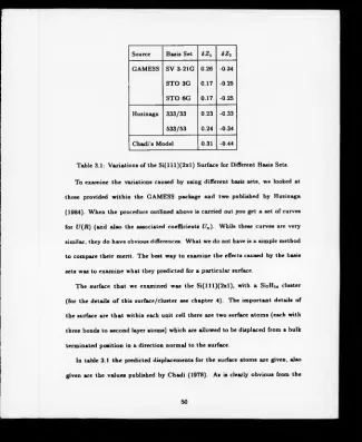
To examine the variations caused by using different basis sets, we looked at

three provided within the GAMESS package and two published by Huzinaga

(1984). When the procedure outlined above is carried out you get a set of curves

for U(R) (and also the associated coefficients Un)- While these curves are very

similar, they do have obvious differences. What we do not have is a simple method

to compare their merit. The best way to examine the effects caused by the basis

sets was to examine what they predicted for a particular surface.

The surface that we examined was the S i(lll)(2 x l), with a SiyHu cluster

(for the details o f this surface/cluster see chapter 4). The important details of

the surface are that within each unit cell there are two surface atoms (each with

three bonds to second layer atoms) which are allowed to be displaced from a bulk

terminated position in a direction normal to the surface.

In table 3.1 the predicted displacements for the surface atoms are given, also

given are the values published by Chadi (1978). As is clearly obvious from the

results, there are systematic variations from one type of basis set to another. We

decided to proceed using the basis sets published by Huzinaga (1984) for two

reasons; the Huzinaga basis sets gave the results that were the closest to Chadi’s

result, and they are available for a very wide range o f elements.

Chapter 4

Cluster Construction.

“There is something fascinating about science. One gets such wholesale

returns o f conjecture out of such a trifling investment o f fact.”

— Mark Twain, Life on the Mississippi.

4.1

In tro d u ctio n .

“If the chemist’s view o f bonding its a local phenomenon is correct, then the

understanding of adsorbate-surface bonding should be tractable to the cluster

model approach” (Messner, 1979). The experience of quantum chemists is that

this is a valid assumption for covalently bonded crystals, therefore we will aim to

develop clusters to be used within the tight-binding model.

We are in heed o f a systematic method to construct the clusters that will be

needed to represent an infinite surface. A review o f the literature shows that in

general quantum chemists work only with ‘minimal clusters’ , i.e. those which rep­

resent only one surface cell (Barone, 1987; Nishida, 1978; Redondo, 1977). Those

that do work with larger clusters appear not to have a systematic method of se­

lecting their clusters (Swarts, 1981). The aim o f the work presented in this chapter

is to set out such a systematic method of cluster construction and enlargement.

There are a number of things that any scheme should aim to achieve or take into

account;

• Correct local bonding o f displaced atoms,

• Surface stoichiometry,

• Pseudo-surfaces,

• Cluster enlargement and convergence o f results with increasing cluster size.

The rest o f this chapter will be split into the following sections; a consideration

o f the construction of minimal clusters, the treatment o f pseudo-surfaces, cluster

enlargement and convergence.

4.2 C on stru ction o f M inim al Clusters.

To consider the construction of a minimal cluster, let us start with the following

assumptions; that all the atoms are in their bulk terminated positions (i.e. there

is no reconstruction or relaxation) with bulk like bonding, and a minimal cluster

represents a single surface unit cell. We are now in a position to use some details of

the surface under consideration, in particular which crystal face and the expected

reconstruction pattern, e.g. the S ilicon (lll) surface with a (2x1) reconstruction

pattern. As a first approximation let us identify only those atoms within a unit cell

O S u r f a c e A to m ^ 2 n d L a y e r A tom

U n it C e ll B o u n d a r y

Figure 4.1: The S i(lll)(2 x l) surface assuming a bulk terminated crystal,

which might be expected to undergo large displacements from their bulk termi­

nated position. In the case of the S i(lll)(2 x l) surface (see ligure 4.1), one might

expect only the two surface atoms to be displaced perpendicular to the surface.

Since this is a minimal cluster, we will necessarily have the correct stoichiometry.

To obtain the correct local bonding, one needs to add additional atoms in their

bulk positions, which will remain fixed throughout the calculations. In figure 4.2

are shown the minimal clusters for the three surfaces that will be used to test the

method, namely, S i(lll)(2 x l), Si(100)(2xl) and G aAs(110)(lxl).

4.3

P seu do-Su rfaces.

When we use a cluster to represent the electronic structure o f an infinite or semi­

infinite system, we necessarily introduce unwanted effects due to the “pseudo­

surface” associated with the boundary of the cluster. Since the whole basis of

using clusters to model the electronic structure of a crystal depends on the ideal

that bonding is a local effect, it is essential that any edge effects are small. However

Si( 111 )(2x 1)

QJ 1st Layer

^ 2 n d Layer

- - - Unit Cell Boundary

S i(1 0 0 )(2 x 1 ) G a A s ( 1 1 0 ) ( 1 x 1 )

Figure 4.2: Minimal clusters for the S i(lll)(2 x l), Si(100)(2xl) and GaAs(llO)-

( lx l ) surfaces.