University of Warwick institutional repository: http://go.warwick.ac.uk/wrap
This paper is made available online in accordance with
publisher policies. Please scroll down to view the document
itself. Please refer to the repository record for this item and our
policy information available from the repository home page for
further information.
To see the final version of this paper please visit the publisher’s website.
Access to the published version may require a subscription.
Author(s): Laurent Badel , Sandrine Lefort, Thomas K. Berger, Carl C.
H. Petersen, Wulfram Gerstner and Magnus J. E. Richardson
Article Title: Extracting non-linear integrate-and-fire models from
experimental data using dynamic I–V curves
Year of publication: 2008
Link to published version:
http://dx.doi.org/
10.1007/s00422-008-0259-4
Biol Cybern (2008) 99:361–370 DOI 10.1007/s00422-008-0259-4
O R I G I NA L PA P E R
Extracting non-linear integrate-and-fire models
from experimental data using dynamic I –V curves
Laurent Badel · Sandrine Lefort · Thomas K. Berger · Carl C. H. Petersen · Wulfram Gerstner · Magnus J. E. Richardson
Received: 4 July 2008 / Accepted: 11 September 2008
© The Author(s) 2008. This article is published with open access at Springerlink.com
Abstract The dynamic I –V curve method was recently
introduced for the efficient experimental generation of redu-ced neuron models. The method extracts the response properties of a neuron while it is subject to a naturalistic sti-mulus that mimics in vivo-like fluctuating synaptic drive. The resulting history-dependent, transmembrane current is then projected onto a one-dimensional current–voltage relation that provides the basis for a tractable non-linear integrate-and-fire model. An attractive feature of the method is that it can be used in spike-triggered mode to quantify the dis-tinct patterns of post-spike refractoriness seen in different classes of cortical neuron. The method is first illustrated using a conductance-based model and is then applied experimen-tally to generate reduced models of cortical layer-5 pyramidal cells and interneurons, in current and injected-conductance protocols. The resulting low-dimensional neu-ron models—of the refractory exponential integrate-and-fire
L. Badel (
B
)·W. GerstnerLaboratory of Computational Neuroscience, School of Computer and Communications Sciences and Brain Mind Institute, Ecole Polytechnique Fédérale de Lausanne (EPFL), 1015 Lausanne, Switzerland
e-mail: [email protected]
T. K. Berger
Laboratory of Neural Microcircuitry, Brain Mind Institute, Ecole Polytechnique Fédérale de Lausanne (EPFL), 1015 Lausanne, Switzerland
S. Lefort·C. C. H. Petersen
Laboratory of Sensory Processing, Brain Mind Institute, Ecole Polytechnique Fédérale de Lausanne (EPFL), 1015 Lausanne, Switzerland
M. J. E. Richardson
Warwick Systems Biology Centre, University of Warwick, Coventry CV4 7AL, UK
e-mail: [email protected]
type—provide highly accurate predictions for spike-times. The method therefore provides a useful tool for the construction of tractable models and rapid experimental classification of cortical neurons.
Keywords I-V curve·Exponential integrate-and-fire· Refractoriness
1 Introduction
The appropriate level of detail in a biophysical neuron model is set by its functional requirements. From the perspective of detailed ion-channel models, the Hodgkin–Huxley
formalism (Hodgkin and Huxley 1952), comprising
redu-ced models of the kinetics of voltage-gated channels with averaged activation and inactivation variables, represents a gross simplification. However, in the context of causally lin-king cellular electrophysiology to the broad features of ion-channel makeup, the formalism is highly satisfactory. At the next scale up in the modeling of neural tissue, a cen-tral goal is to predict emergent computational properties in populations and recurrent networks of neurons (Gerstner and van Hemmen 1993;Brunel and Hakim 1999;Gerstner 2000;
Brunel and Wang 2003;Gigante et al. 2007) from the pro-perties of their component cells. The neurons that comprise such network models may be modeled in biophysical and geometric detail (Koch 1999; Huys et al. 2006) for large-scale simulation (Markram 2006), but also of great practical use are experimentally-verifiable reduced descriptions that allow for a transparent understanding of the causal relation between cellular properties and network states.
the context of neurons the dimensionality arises both from their extended geometry and the coupled non-linear diffe-rential equations that describe the voltage-gated channels. Reduction schemes typically consider the neuron to be isopotential (a point neuron) and simplify the voltage-history dependent channel dynamics by a one-dimensional relation between current and voltage or a two-dimensional relation capturing effects from an additional subthreshold or
adap-tation current (Brunel et al. 2003;Richardson et al. 2003;
Izhikevich 2004;Gigante et al. 2007).
Integrate-and-fire (IF) neurons [seeBurkitt(2006a,b) for
a recent review] underlie many forms of reduced model and comprise a voltage-derivative coming from the capacitive
C charging of the membrane and some choice of
voltage-dependent function F(V)which aims to capture the
voltage-dependent ionic current
dV
dt =F(V)+Iapp/C. (1)
Here Iappis any current injected by an intracellular electrode.
The action potential in IF models is modeled by a threshold
Vt h (at low or high voltage depending on the particular IF
model) and a reset Vr efollowed by a refractory period, after
which the subthreshold dynamics of Eq. (1) continue.
The most commonly used member of the IF family is the linear Leaky IF model (LIF) that features an ohmic form
F(V)=(Em−V)/τm, where Emis the rest andτmthe
mem-brane time constant, with a low threshold Vt h ∼ −50 mV
considered to be at the onset of the spike. This model is lar-gely tractable and has been extensively studied in the context
of both populations and networks (Brunel and Hakim 1999;
Gigante et al. 2007) of neurons. However, the lack of an explicit spike mechanism in the LIF is a weakness and can lead to responses that are not common to the general class of Type I neurons, particularly in relation to the response
to fluctuating input (Fourcaud-Trocmé and Brunel 2005).
The canonical type I neuron can be cast in the IF form—
the Quadratic IF (QIF) model—with a function F(V)that
is parabolic (Ermentrout and Kopell 1986). More recently
a second non-linear model, the Exponential IF model, was
introduced (Fourcaud-Trocmé et al. 2003) that captures the
action potential in a more biophysically-motivated way by fit-ting the region of the spike-onset to the conductance-based
Wang–Buzsáki model (Wang and Buzsáki 1996). Though the
response properties of such non-linear IF models do not in general have solutions in terms of tabulated functions, they can nevertheless be extracted numerically but exactly via a
simple algorithm (Richardson 2007). Therefore, the family
of non-linear IF neurons provides a tractable class of reduced model which, if matched to experiment, provide an excellent starting point for the causal analysis of emergent states in recurrent network models.
In this paper, we will review the dynamic I –V method (Badel et al. 2008) which provides an efficient technique for extracting non-linear IF models and post-spike refractory response-functions from intracellular voltage recordings. The method will be illustrated using the conductance-based Wang–Buzsáki hippocampal interneuron model. It will then be applied to intracellular voltage recordings from cortical neurons to build reduced models of layer-5 pyramidal cells and interneurons. It will be further demonstrated that the method can be used in dynamic-clamp conductance-injection mode in which the shunting effects of synaptic inhibition on voltage fluctuations are included. The paper closes with a discussion of the applications and extensions of the method.
2 From dynamic I –V curves to reduced models
The potential across the neuronal membrane obeys a current balance equation
CdV
dt +Iion=Iapp (2)
where V is the membrane voltage at the point of the applied
current Iapp (in this paper, the soma), C is the membrane
capacitance and Iioncontains the intrinsic voltage-gated
cur-rents that are instantaneous-voltage and voltage-history dependent. In general neurons are not sufficiently compact for the voltage to be constant throughout the cell. Therefore, the voltage and currents must be interpreted as being some measure of the properties within, roughly speaking, an elec-trotonic length of the electrode. Hence, in an experimental
context the ionic current Iion will also include lateral
cur-rents flowing from the soma to the axon or dendrites. The applied current that is injected into the cells is a fluctuating waveform (combination of Ornstein–Uhlenbeck processes) chosen to create voltage traces that are in-vivo-like in that they fluctuate and explore the entire range of subthreshold voltages.
To provide a clear demonstration of the dynamic I –V methodology it is first applied to a conductance-based
neu-ron model—the Wang–Buzsáki model (Wang and Buzsáki
1996)—for which the underlying properties are known. In
this model the ionic transmembrane currents take the form
Iion=gL(V −EL)+gN am3h(V −EN a)
+gKn4(V−EK), (3)
wheregL,gN a,gKare the maximum leak, sodium and
potas-sium conductances, EL, EN a, EKthe corresponding reversal
potentials, and m, h, n are gating variables. The time course of
the ionic current Iion, due to some pattern of applied current
Biol Cybern (2008) 99:361–370 363 0 20 Iapp (pA) -90 -60 -30 0 30 V (mV)
0 100 200
t (ms) 0
Iion
(pA)
-90 -80 -70 -60 -50
V (mV) -20 -15 -10 -5 0 5 Iion (pA)
0.1 1 10
Ce (pF)
1 10 100 var[I app - C e dV/dt]
-80 -70 -60 -50
V (mV) -2 0 2 4 6 8 10 F(V) (mV/ms)
-80 -60 -40 -20 V (mV) 0.01 0.1 1 10 100
F(V) + (E
m - V)/ τm -70 -50 V (mV) -70 -50 V (mV) -70 -50 V (mV) -5 0 5 10 F(V) (mV/ms) -70 -50 V (mV)
0 100 200 300
0 0.2 0.4 0.6 0.8 1 1/ τm (1/ms)
0 100 200 300
-80 -76 -72 -68 -64 -60 Em (mV)
0 100 200 300
-70 -60 -50 -40 VT (mV)
0 100 200 300
0 2.5 5 7.5 10 ∆T (mV) Experiment rEIF model A B C D
Time following spike (ms)
5-10ms 10-20ms 20-30ms 30-50ms
pre-spike I-V data E
F
G
5-10ms 10-20ms 20-30ms 30-50ms
[image:4.595.55.541.60.351.2]50ms 20mV
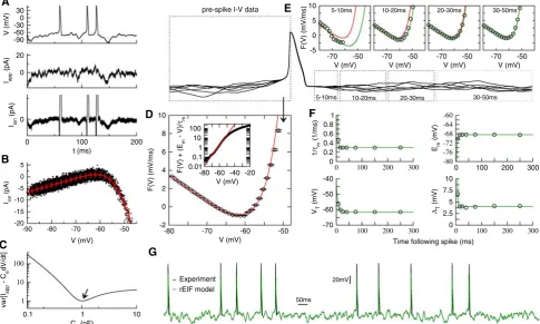
Fig. 1 Summary of the dynamic I –V curve method and its application
to the Wang–Buszáki model. a The derivative of the membrane voltage (top graph), multiplied by the cellular capacitance, is subtracted from the injected current (middle graph) to yield the intrinsic membrane cur-rent Iion(bottom graph). b The intrinsic membrane current Iionis plotted
against the membrane voltage (black symbols). The dynamic I –V curve (red symbols) is obtained by averaging Iionin small voltage bins. Error
bars represent the standard deviation. c Measuring the cellular capaci-tance. At a fixed subthreshold voltage, the dynamic membrane current
Iion =Iapp−CdV/dt has a variance that depends on the value of C
used in the calculation; the correct value of C corresponds to the point of minimal variance. d Relating dynamic I –V curves and non-linear integrate-and-fire models. The function F(V)= −Idyn(V)/C (sym-bols) is plotted as a function of voltage, together with the EIF model
fit (red line). Inset: semi-log plot of F(V)with leak current subtracted, showing a nearly exponential run-up. e Spike-triggered dynamic I –V curves. The functions F(V)measured in small time slices after each spike (symbols) are plotted together with the the EIF fit (green) and the pre-spike I –V curve as a reference (red). At early times it is clearly seen that both the conductance and the spike threshold are significantly increased. f Dynamics of the EIF model parameters during the refrac-tory period. The parameters obtained from the fits of the I –V curves in e are plotted as a function of the time since the last spike (symbols) and fitted with exponential functions (green). g Comparison of the pre-diction of the refractory EIF (rEIF) model (green) with a voltage trace of the Wang–Buzsáki model (black) shows excellent agreement, with 96% of the spikes correctly predicted by the EIF model within a 5 ms window
Eq. (2) to give
Iion=Iapp−C
dV
dt . (4)
If the capacitance C is known (to be derived in a following section) and the voltage derivative calculated directly from finite-differences, all quantities on the right-hand side of the
equation are known and so the required Iionis obtained as a
function of time. This process is shown in Fig.1a.
Definition of the dynamic I –V curve The measured voltage
and ionic current derived from Eq. (4) represent a current–
voltage relation parameterized by time. The aim is to find a one-dimensional relation between current and voltage and
so a scatter plot is made of Iion as a function of voltage,
with all points that lie within 200 ms after an action potential excluded (the post-spike refractory behavior is returned to
later). The average of Iionfor a particular voltage
Idyn(V)= Iion(V,t)V (5)
defines the dynamic I –V curve Idyn. This quantity is plotted
in Fig.1b where it can be seen that the dynamic I –V curve
Determining the membrane capacitance Capacitance can be
measured in a variety of ways, with the standard approach in current-clamp mode being the fitting of the early vol-tage response to rectangular current pulses. However, applied fluctuating-current protocols offer a convenient alternative
method that is now described: If Eq. (4) is applied with an
estimate Ceof the capacitance instead of its true value C, an
incorrect estimate of the ionic current Iionis found that, at a
fixed voltage V , has a variance of the form
Var
Iion
Ce
V =Var
Iion
C
V +
1
C −
1
Ce
2
VarIapp
V (6)
where Var[X]Vdenotes the variance of some quantity X
mea-sured at a voltage V , and where it is assumed that there is no covariance between applied and ionic currents (justifiable in the ohmic region of the I –V curve and consistent with the standard method for measuring capacitance). The true mem-brane capacitance will therefore correspond to the estimate
Ce which minimizes the right-hand side of Eq. (6)
evalua-ted in some voltage range where the I –V curve is linear (in
practice±1 mV from the resting potential). The quantity C
can also be found directly by solving Eq. (6) for C to yield
C= Var
Iapp
V
CovardVdt,Iapp
V
(7)
where again, these two quantities are measured near a
vol-tage where the I –V curve is ohmic. Equations (6) and (7)
applied to the Wang–Buzsáki model in Fig.1c yield a value
of C=1.018µF/cm2, which is very close to the true value of
C=1µF/cm2.
Fitting to a non-linear IF model The dynamic I –V curve
provides a direct mapping between the membrane voltage and the mean instantaneous value of the membrane current, which can be related to the template for non-linear IF
neu-rons with the interpretation that F(V)= −Idyn(V)/C. This
is shown in Fig.1d in which the measured F(V)(minus the
dynamic IV curve divided by capacitance) is clearly seen to comprise a linear ohmic component in the subthreshold
vol-tage range−90 to−60mV followed by a sharp exponential
rise from−60 mV (this is clearly seen in the inset). This form
suggests that the exponential integrate-and-fire neuron
F(V)= 1
τm
EL−V +∆Te(V−VT)/∆T
(8)
could potentially provide an accurate fit. Such a fit, with
para-meters EL = −68.5 mV,τm =3.3 ms, VT = −61.5 mV and
∆T =4.0 mV, is plotted in Fig.1d in red and shown to be
highly satisfactory.
Post-spike response and refractoriness It can be anticipated
that the transient activation of ionic conductance during an action potential can alter significantly the cellular response
during the refractory period. These changes in response pro-perties can be investigated by examining the ‘spike-triggered’ dynamic I –V curves, i.e., the I –V curves measured in small
time slices after a spike (Fig. 1e). Although the Wang–
Buzsáki model displays relatively little refractoriness, it is possible to fit again the post-spike I –V curve to the EIF
form in Eq. (8), yielding a different set of the parameters
τm, EL, VT and∆T for each of the time slices. These new
values define for each parameter a dynamics parametrized
by the time since the last output spike (Fig.1f).
Refractory EIF model A refractory extension of the basic
EIF model (called the rEIF model), can be obtained by fit-ting the post-spike dynamics of the EIF model parameters
plotted in Fig.1f. In the case of the Wang–Buzsáki model,
all parameters could be fitted with a single exponential func-tion, resulting in the following model
dV
dt =F(V, τm,EL,VT, ∆T)+
Iapp
C . (9)
1
τm = 1
τ0
m +aτ−1
m e
−(t−tsp)/τ τ−1
m (10)
EL =EL0+aELe−(
t−tsp)/τE L
(11)
VT =VT0+aVTe−(
t−tsp)/τ
VT (12)
∆T =VT0+a∆Te−(
t−tsp)/τ
∆T (13)
where the function F is defined by Eq. (8), tsp is the time
of the last spike, and the superscript ‘0’ in (10)–(13) denotes
the pre-spike value of a parameter. In the present application, the ultimate voltage threshold (at the top of the spike) was
taken to be Vt h = +30 mV, and the voltage reset taken to
be the average voltage at the end of the refractory period,
Vr e = −71.2 mV. The refractory period was taken slightly
longer than the typical duration of a spike (we usedτref =
8 ms for the case of the WB model). An example trace of
this model is compared in Fig. 1g with the output of the
Wang–Buzsáki model generated with the same input current, showing excellent agreement in both the subthreshold region and the timing of spikes, with 96% of correctly predicted spikes at 5 ms precision (2 spikes out of 55 were missed). Note that we do not evaluate here the performance of the normal EIF model with threshold and reset, which was addressed in
our previous publication (Badel et al. 2008) and gives results,
for physiological firing rates (<10 Hz) that are close to those of the refractory model.
2.1 Results for cortical pyramidal cells
Figure2summarizes our previous results for cortical
pyrami-dal cells. In Fig.2a the intrinsic currents are plotted against
the membrane voltage. The scatter plot of the intrinsic
cur-rent shown in Fig.2a exhibits similar features as observed for
Biol Cybern (2008) 99:361–370 365
-80 -60 -40
V (mV) -2000 -1500 -1000 -500 0 500 Iion (pA) experiment rEIF model
-80 -60 -40 -20
-2 0 2 4
-80 -60 -40 -20
-2 0 2 4
0 5 10 15 20
neuron firing rate (Hz) 0
5 10 15 20
model firing rate (Hz)
0 50 100
performance/reliability (%)
count
-70 -60 -50 -40 -30
V (mV)
P(V)
-80 -60 -40 -20
-2 0 2 4
-80 -60 -40 -20
Voltage (mV) -2
0 2 4
0 100 200 300
0.05 0.1 0.15 1/ τm (1/ms)
0 100 200 300
-40 -35 -30 -25 VT (mV)
0 100 200 300
-60 -58 -56 -54 Em (mV)
0 100 200 300
0 1 2 3 ∆T (mV)
-500 0 500
I ion (pA)
0 100 200 300 400
Cpulse (pF)
0 100 200 300 400 CdIV (pF)
-80 -60 -40
V (mV) 0
5 10
F(V) (mV/ms) -40 -20
V (mV) 0.01 0.1 1 10 100
F(V) + (E
m
-V)/
τm
0 20 40
τm (ms)
-70 -60 -50 -40
EL (mV)
0 10 20 30
VT - EL (mV)
0 2 4
∆T (mV)
5-10ms 10-20ms 20-30ms 30-50ms D E F H
A B C
G
time since last spike (ms) time since last spike (ms) time since last spike (ms) time since last spike (ms)
[image:6.595.55.539.52.362.2]F(V) (mV/ms)
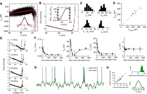
Fig. 2 Application of the dynamic I –V method to layer-5 pyramidal
cells. a The intrinsic membrane current is plotted against the mem-brane voltage (black symbols). The dynamic I –V curve (red) is clearly seen to comprise a linear component in the subthreshold region fol-lowed by a sharp activation in the region of spike initiation. Inset: Examination of the variance of Iion near the resting potential in the
absence (black) or presence (red) of injected current suggest that the majority of the variance comes from intrinsic noise. b The function
F(V)= −Idyn(V)/C is plotted here (symbols) together with the EIF
model fit (red). Inset: The exponential rise of the spike generating current is shown in a semi-log plot of F(V)with the leak currents subtracted. c Histograms of the EIF model parameters for a sample (N =12) of pyramidal cells, showing considerable heterogeneity in the response properties of neurons in this population. d The cellular capacitance calculated with our optimization method (see text) is com-pared to the result of the standard current-pulse protocol, showing a
good agreement between the two methods. e Spike-triggered dynamic
I –V curves. The I –V curves measured in small time slices after a spike
are plotted together with the EIF fit (green) and the pre-spike I –V curve as a reference (red). f Post-spike dynamics of the EIF model parame-ters (symbols) together with the fits to an exponential model. While conductance and spike threshold could be accurately fitted with a single exponential, the variation in the equilibrium potential ELrequired two exponential components for a good fit. The spike width∆T did not vary significantly for these cells. g Comparison of the prediction of the rEIF model (green) with experimental data shows good agreement in the subthreshold region and in the prediction of spike times. h Summary of the performance of the rEIF model for the 12 cells investigated. Left: Prediction of the firing rate. Top right: Histogram of the performance measure. Bottom right: Voltage distribution for the rEIF model (green) and the experimental data (black). The figure is adapted from (Badel et al. 2008)
variability around the mean. Two processes can be identi-fied that could contribute to this variability: (i) the projection of a time-dependent quantity on the instantaneous voltage
whereas the ionic current Iionis a function dominated by the
voltage history due to the activation of voltage gated cur-rents, or (ii) the amplification of the background noise due
to the voltage derivative in Eq. (4). As the dynamic I –V
curve can be expected to give an accurate approximation of the intrinsic membrane current only if the contribution from point (i) above is relatively insignificant, it is important to weigh the relative contribution of these two possible sources of variance. This can be investigated by examining the
dis-tribution of Iionmeasured when there is no injected current
and the voltage is at its rest, and comparing the distribution when the voltage is fluctuating triggered to the same value of
the voltage. This comparison is shown in the inset to Fig.2a
where it can be seen that the distribution of Iionwhen the
vol-tage is at rest (black lines) accounts for a significant propor-tion (83% of the standard deviapropor-tion) of the spread when the voltage has a dynamics; this suggests that the overwhelming proportion of the variability is due to point (ii) above—the amplification of noise from the voltage derivative—and that
the underlying relation between Iionand voltage is relatively
The pre-spike I –V curves were very well fitted by the EIF
model. However, as is clearly seen in Fig.2a,b, at the onset
of the spike the rise in the I –V curve is much sharper than
is observed in the Wang–Buzsáki model (with parameter∆T
of the order of 1–2 mV, see Fig.2c), and remains very close
to exponential over almost 4 decades (Fig.2b, inset). The
range of parameters obtained for the 12 measured pyramidal
neurons, shown in Fig.2c, suggests a significant degree of
heterogeneity in this population of cortical neurons. As regards the measurement of the cellular capacitance,
the values obtained using Eq. (7) were consistent across
dif-ferent voltage traces from the same cell, with a coefficient of
variation of the order of a few percent. The validity of (7) was
further tested by comparing with the values obtained by using the standard protocol of measuring the cellular capacitance from the voltage response to small current pulses. For the latter the capacitance was estimated by fitting the response with an exponential and averaging over 4 trials. As is shown
in Fig.2d, there is a good agreement between the results of
the two methods. Overall, the measured pyramidal cells
exhi-bited relatively high capacitance values (250±75 pF, n=12
cells).
In contrast to the Wang–Buzsáki model, pyramidal cells
showed a long refractory period (up to ∼100 ms) during
which the cellular response changed considerably. This is seen very clearly in the post-spike I –V curves shown in
Fig2e. Interestingly, the post-spike I –V curves could still be
fitted to the EIF form in Eq. (8) allowing refractory properties
to be described in terms of the simple rEIF model (9)–(13).
The dynamics of the parameters are plotted in Fig.2f for one
example cell, and consistently comprised: an increase in the
leak conductancegL, a biphasic response in the effective rest
voltage and, importantly, a significant increase in the spike
threshold VT. For pyramidal cells relatively little change was
seen in the spike width∆T.
In terms of predictive power, the rEIF model derived from fits to the steady-state and spike-triggered I –V curves was highly satisfactory, with an average 83% of succesfully pre-dicted spikes within a 5 ms window, relative to the instrinsic reliability of the cells.
3 GABAergic interneurons
One of the potential applications of the dynamic I –V curve is the rapid classification of cell type and response proper-ties. To test whether different cell classes could be identi-fied on the basis of their dynamic I –V curve and refractory properties, we applied our method to cortical GABAergic interneurons, and compared with the results obtained for pyramidal cells. The results for interneurons are
summari-zed in Fig.3. In general, the dynamic I –V curve for these
interneurons was surprisingly similar to those observed in
pyramidal cells, particularly for the response properties in the run up to the spike. For this cell type also the exponential
integrate-and-fire model (8) matched the I –V curves
accura-tely as can be seen in Fig.3a and with similar distributions of
the parameters (except for the lower membrane time constant
τm) as seen in Fig.3b. For the refractory properties (Fig.3c)
the behavior of the rest EL was notably different from the
pyramidal case and did not show the biphasic response seen
in Fig.2b but rather a simple exponential relaxation from a
hyperpolarized reset. The other parameter that distinguished
the two cell types was the cellular capacitance (250±75 pF
for pyramidal cells, n =12, and 94±21 pF for interneurons,
n = 6) which is consistent with the smaller interneurons.
Although the variability in membrane time constant was less significant than previously found for pyramidal cells (with a CV of 12% as opposed to 32% for pyramidal cells), the other cellular parameters showed considerable scatter (with
CVs of 22% for the distance to threshold VT − EL, and
27% for the spike width ∆T), suggesting a high degree of
inhomogeneity also in this population. It can also be noted
that the transient increase in the spike onset VT is smaller
for this fast-spiking cell (∼4 mV) than seen in the pyramidal
cell∼15 mV. In terms of model performance, the predictions
of the corresponding rEIF models were again excellent (in fact marginally better than for pyramidal cells) with an ave-rage 96% of correctly predicted spikes relative to the intrinsic reliability of the cells.
4 Application to conductance injection protocols
The dynamic I –V method can also be employed to des-cribe the voltage dynamics of pyramidal cells under dynamic-clamp conductance injection. To demonstrate this, we injected layer-5 pyramidals with a mixture of excitatory and inhibitory fluctuating conductances modeled as Ornstein–
Uhlenbeck processes with two distinct correlation timesτe=
2 ms andτi =10 ms. For conductance injection the applied
current is given by
Iapp(t)=ge(t)(Ee−V(t))+gi(t)(Ei−V(t)), (14)
where ge andgi are the excitatory and inhibitory
conduc-tance waveforms, and the synaptic reversal potentials are
given by Ee = −10 mV and Ei = −70 mV. In this case,
the dynamic I –V curve was qualitatively similar to the case of current injection. However, a second, slow exponential activation was needed to accurately fit the I –V curve. This
is shown in Fig.4a where the function F(V)was modeled
as
F(V)=1 τm
EL−V+∆Te(V−VT)/∆T+∆Te(
V−VT)/∆T.
Biol Cybern (2008) 99:361–370 367
-100 -75 -50
V (mV) 0
5 10 15
F(V) (mV) -45 V (mV)-40 -35 datarEIF model
1 10 100
F(V) + (E
m
- V)/
τm
-70 -60
EL (mV)
0 100 200 300
time following spike (ms) 0.1
0.12 0.14 0.16 0.18 0.2
1/
τm
(1/ms)
0 100 200 300
time following spike (ms) -70
-68 -66
Em
(mV)
0 100 200 300
time following spike (ms) -46
-45 -44 -43 -42 -41 -40 -39
VT
(mV)
0 100 200 300
time following spike (ms) 0
5 10
∆T
(mV)
0 10 20
τm (ms)
0 10 20 30
VT - EL (mV)
0 2 4 6
∆T (mV)
0 20 40 60 80 100 performance/reliability ratio (%)
0 5 10 15 20 25 30 neuron firing rate (Hz) 0
5 10 15 20 25 30
model firing rate (Hz)
100ms 10mV
A E
D
C
[image:8.595.59.541.55.290.2]B
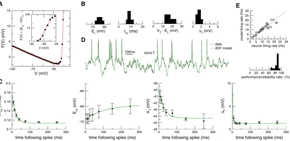
Fig. 3 GABAergic cortical interneuron models derived using the
dyna-mic I –V methodology. a The function F(V)= −Idyn(V)/C for a
fast-spiking interneuron is plotted (symbols) together with the EIF model fit (red). Inset: The exponential rise of the spike generating current is shown in a semi-log plot of F(V)with the leak currents subtracted.
b Distribution of the EIF model parameters for a sample (N =6) of interneurons. The histograms overlap significantly with those of pyra-midal cells shown in Fig2. c Post-spike dynamics of the EIF model parameters (symbols) together with the fits to an exponential model.
In the case of cortical interneurons all parameters could be fitted satis-factorily with a single exponential. Note that the transient, post-spike increase in the spike onset VT (∼4 mV) is smaller in this fast-spiking interneuron than that for pyramidals (∼15 mV—see Fig.2). d Compari-son of the prediction of the rEIF model (green) with experimental data shows close agreement in the subthreshold region and in the predic-tion of spike times. e Summary of the performance of the rEIF model for the 6 cells investigated. Top: Prediction of the firing rate. Bottom: Histogram of the performance measure
The presence of an additional slow exponential component to the activation is likely due to the reduced amplitude of voltage fluctuations (from the diminished effective mem-brane time constant). This resulted in voltage trajectories that were concentrated close to the region of spike initia-tion, making a more detailed description of action potential onset dynamics necessary in order to correctly predict the timing of spikes. The analysis of the refractory properties yielded results consistent with the case of current injection, with changes in the membrane time constant, equilibrium potential and spike initiation threshold. For simplicity, the
parameters∆T, VT −VT and∆T were taken as constant in
the fitting of the post-spike I –V curves (Fig.4b).
The accuracy of the model at predicting spike timing for this particular example was slightly lower than in the current-clamp case. Overall, 63% of action potentials were correctly predicted within a 5 ms window, whereas on average 83% were correctly predicted in the current-clamp case, com-pared to the intrinsic reliability of the cells (see Appen-dix). Although the data set, comprising only one pyramidal cell, does not allow for a systematic analysis of the perfor-mance, these results clearly demonstrate the applicability of the dynamic I –V curve method to conductance injection pro-tocols.
5 Discussion
We used the dynamic I –V curve method to characterize the response properties of neocortical layer-5 pyramidal cells and GABAergic interneurons in current-clamp mode and additio-nally demonstrated that the method can be used in dynamic-clamp conductance-injection protocols. For interneurons, we found that the dynamic I –V method yields results of similar quality to those previously reported for pyramidal cells. In particular, we find that the refractory exponential integrate-and-fire model is able to predict both the subthreshold voltage and the timing of spikes highly accurately. The fast-spiking interneuron was characterized by a smaller cellular
capaci-tance (∼100 pF) than pyramidals, a shorter membrane time
constant (∼10 ms) and the lack of a biphasic response in the
effective equilibrium potential during the refractory period. Other parameters showed significant overlap with the values obtained for pyramidal cells and a similar spread of para-meter values in the studied sample of interneurons was also seen.
-50 V (mV) 0
5 10 15
F(V) (mV/ms)
10mV data rEIF model -50 -40 -30
V (mV) 1 10 100
F(V) + (E
m
- V)/
τm
0 100 200
time following spike (ms) 0.1
0.15 0.2 0.25
1/
τm
(1/ms)
0 100 200
time following spike (ms) -68
-66 -64 -62 -60 -58 -56
Em
(mV)
0 100 200
time following spike (ms) -45
-40 -35 -30 -25
VT
(mV)
100ms
A B
[image:9.595.56.542.53.289.2]C
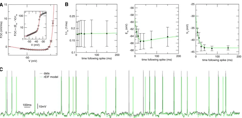
Fig. 4 Application of the dynamic I –V method with conductance
injection. a The function F(V)= −Idyn(V)/C is plotted (symbols)
together with the fit (red) to the function(14). Inset: Two exponential components are clearly seen in a semi-log plot of F(V)with the leak currents subtracted. b Post-spike dynamics of the EIF model parame-ters (symbols) together with the fits to an exponential model. The
time-dependent resting potential shows a clear biphasic response as was seen for layer-5 pyramidals in the current-injection protocol. c Comparison of the prediction of the rEIF model (green) with experimental data again shows good agreement in the subthreshold region and in the prediction of spike times
reports of ‘kink’-like spike initiation (Naundorf et al. 2006;
McCormick et al. 2007). Second, the Wang–Buzsáki model showed very little refractoriness in contrast to the experimen-tal data where the refractory properties were more pronoun-ced and lasted significantly longer. It would be interesting to determine how much this discrepancy is accounted for by the presence of additional voltage-gated channels such as adaptation currents or by the extended spatial structure of neurons. As a related point, it would be interesting to inves-tigate the influence of multiple action potentials on the dyna-mics of the EIF model parameters. In this paper, only the influence of the last action potential was considered. Howe-ver, it is possible that multiple-spike effects will dominate the response at higher firing rates.
In the case of dynamic-clamp conductance injection we found that the I –V curve was best fitted by a non-linear integrate-and-fire model that comprised two exponential components: the sharp exponential activation associated with the spike-generating sodium current is preceded by a slow inward rectification that is also very close to exponential. The model derived from the I –V curve was also able to predict the timing of spikes with a satisfactory level of accuracy com-pared with the intrinsic reliability of the neuron, although for this cell the model performance was marginally lower than typically obtained in the current clamp case. The proximity of
the trajectories to the threshold for the example treated here suggests that the lower performance might be attributable to the oversimplified description of action-potential onset dynamics that is inherent in the one-dimensional EIF model. This is backed up by preliminary analysis we have performed on a model that includes inactivation of the sodium current (details not shown). Further experiments would be needed to verify this hypothesis.
Also seen was that the substantial degree of inhomoge-neity in the response properties, previously observed for
pyramidal cells (Badel et al. 2008), was also found here for
cortical interneurons. Since the majority of network-level models assume identical properties for component cells, it would be interesting to investigate how the presence of inho-mogeneities could affect collective behaviors, such as
transi-tions to oscillatory states (Brunel and Hakim 1999;Gigante
et al. 2007), in networks of excitatory and inhibitory neurons.
Transient increase in spike onset A key aspect of the
refrac-tory response quantified by the dynamic I –V curve methodo-logy was the transient increase in the spike-onset parameter
VT following an action potential. Though this feature was
Biol Cybern (2008) 99:361–370 369
VT 0and the additional transient increase as VT 1we have,
loo-king at Figs.2f and3c, for pyramidal cells a typical distance
to threshold of VT 0−EL∼10 mV and a transient increase
of VT 1∼15 mV, whereas for interneurons these quantites are
VT 0−EL∼24 mV and a transient increase of VT 1∼4 mV.
If one compares the relative increase VT 1/(VT 0−EL)for
these two cells we get a value for pyramidals of 150%, but for the fast-spiking interneuron the relative increase is only 17%. This distinction could well underlie the ability of such
fast-spiking cells to emit closely spaced action potentials.
Furthermore, in the context of mathematical approaches to the transient spike-onset, it is worth noting the surprising fact that the two-dimensional system (voltage and dynamic
threshold VT(t)) is fully solvable in certain conditions. The
corresponding equations are
τLV˙ =EL −V +∆Te(V−VT)/∆T (16)
where
VT =VT 0+VT 1e−t/τT (17)
where it is assumed the spike occured at t =0 so that initially
V = Vr e. If the time constants are identicalτL = τT then
a simple transformation W = V −VT 1e−t/τT reduces the
dynamics to an effective one-dimensional EIF model
τLW˙ =EL−W +∆Te(W−VT 0)/∆T (18)
with a constant threshold for spike-onset VT 0and a lower
reset Wr e = Vr e−VT 1. A similar transformation was first
identified for the Leaky IF model (Lindner and Longtin 2005)
where it was also demonstrated that even for cases where
τL = τT a perturbative approach can be used to
calcu-late many of the response properties of Leaky IF neurons with decaying thresholds. It would be worthwhile to further explore the extension of this to the two-variable EIF model
given by Eqs. (16,17) particularly given its simplicity and
direct experimental relevance.
Appendix: Experimental methods
Current-clamp recordings Experimental methods for the
current-clamp protocol were identical for both pyramidal cells and interneurons. Details of the methods are available
in a previous publication (Badel et al. 2008). Briefly, double
somatic whole cell recordings were obtained from layer-5 pyramidal cells and interneurons, with one pipette injecting the current while the other monitored the voltage. The injec-ted current waveforms were construcinjec-ted from two summed
Onstein–Uhlenbeck processes with time constantsτfast =
3 ms,τslow = 10 ms, and a range of means and variances
were explored. All currents were preceded and followed by a 3-second null stimulus used to assess the amount of back-ground noise, and during which two small square current
pulses (one positive and one negative) were applied to allow for the measurement of the cellular capacitance.
Dynamic-clamp recordings For this protocol, we used the
publicly available data from Challenge A of the
Quantita-tive Single-Neuron Modeling Competition [seeJolivet et al.
(2008a,b) for details on the competition and experimental methods]. The data was acquired from a pyramidal neuron of the rat somatosensory cortex via two-electrode somatic patch clamp. The injected current was of the form
Iapp(t)=ge(t)(Ee−V(t))+gi(t)(Ei−V(t)), (19)
where the voltage V(t)was measured in real-time via the
second electrode. The conductance waveforms consisted of
Ornstein–Uhlenbeck processes with correlation timesτe =
2 ms,τi =10 ms; the reversal potentials for excitation and
inhibition were Ee= −10 mV, Ei = −70 mV.
Performance measure To facilitate comparison with
pre-viously published work, we use the ‘coincidence factor’Γ
(Gerstner and Kistler 2002) as a measure of performance. This coefficient takes into account both the overlap between two spike trains and the similarity in the firing rate. It is defi-ned by
Γ = Ncoinc− Ncoinc
0.5(Nmodel+Nneuron)
1
N (20)
where Ncoincis the number of coincidences with precision
∆,Ncoinc = 2 f∆Nneuronis the number of expected
acci-dental coincidences generated by a Poisson process with the
same firing rate f as the neuron, Nneuron and Nmodel are
the number of spikes in the spike trains of the neuron and the
model, andN is a normalization factor. In this paper, only
ratiosΓ /Γare considered, whereΓ evaluates the overlap
between the prediction of the model and a target
experimen-tal spike train, andΓis calculated between the target spike
train and a second experimental recording obtained with the same driving current. Only pairs of trials with an
experimen-tal reliabilityΓ>0.75 were used in the analysis.
Wang–Buzsáki model The Wang–Buzsáki model (Wang and Buzsáki 1996) is defined by
CdV
dt = −gL(V −EL)−gNam
3h(V −
ENa)
−gKn4(V −EK)+Iapp+Inoise (21)
with gating variables n,m and h obeying a first-order
dyna-mics,
for x=n,m,h, andτx(V)=1/(αx(V)+βx(V)), x∞(V)=
αx(V)/(αx(V)+βx(V)), and the rate constants are given by
αm(V)= −
0.1(V+35)
e−0.1(V+35)−1 (23)
βm(V)=4e−(V+60)/18 (24)
αh(V)=0.07e−(V+58)/20 (25)
βn(V)=(1+e−0.1(V+28))−1 (26)
αn(V)= −
0.01(V +34)
e−0.1(V+34)−1 (27)
βn(V)=0.125e−(V+44)/80. (28)
For the conductances and reversal potentials, we usedgNa=
120, ENa =55,gK =36, EK = −72,gL =0.3 and EL =
−68. The term Inoiseis included here to account for intrinsic
background noise, and is modeled as Gaussian white noise,
Inoise=σ ξ(t), whereξ(t) =0,ξ(t)ξ(t) =δ(t−t), and
we tookσ =0.1 to obtain a level of noise that is comparable
to the one observed experimentally.
Acknowledgments MJER acknowledges funding from the Research Councils United Kingdom (RCUK) with whom he holds an Academic Fellowship. The work was partially supported by the European Integra-ted Project FACETS.
Open Access This article is distributed under the terms of the Creative Commons Attribution Noncommercial License which permits any noncommercial use, distribution, and reproduction in any medium, provided the original author(s) and source are credited.
References
Badel L, Lefort S, Brette R, Petersen CCH, Gerstner W, Richardson MJE (2008) Dynamic I –V curves are reliable predictors of natu-ralistic pyramidal-neuron voltage traces. J. Neurophysiol. 99: 656–666
Brette R, Gerstner W (2005) Adaptive exponential integrate-and-fire model as an effective description of neuronal activity. J. Neuro-physiol. 94:3637–3642
Brunel N, Hakim V (1999) Fast global oscillations in networks of integrate-and-fire neurons with low firing rates. Neural Comput. 11:1621–1671
Brunel N, Wang X-J (2003) What determines the frequency of fast net-work oscillations with irregular neural discharges. J. Neurophysiol. 90:415–430
Brunel N, Hakim V, Richardson MJE (2003) Firing-rate resonance in a generalized integrate-and-fire neuron with subthreshold reso-nance. Phys Rev E 67. article-no 051916
Burkitt AN (2006a) A review of the integrate-and-fire neuron model: I. Homogeneous synaptic input. Biol. Cybern. 95:1–19
Gerstner W, Kistler WM (2002) Spiking neuron models. Cambridge University Press, London
Burkitt AN (2006b) A review of the integrate-and-fire neuron model: II. Inhomogeneous synaptic input and network properties. Biol. Cybern. 95:97–112
Ermentrout GB, Kopell N (1986) Parabolic bursting in an excitable sys-tem coupled with a slow oscillation. SIAM J. Appl. Math. 46: 233–253
Fourcaud-Trocmé N, Hansel D, van Vresswijk C, Brunel N (2003) How spike generation mechanisms determine the neuronal response to fluctuating inputs. J. Neurosci. 23:11628–11640
Fourcaud-Trocmé N, Brunel N (2005) Dynamics of the instantaneous firing rate in response to changes in input statistics. J. Comput. Neurosci. 18:311–321
Gerstner W, van Hemmen JL (1993) Coherence and incoherence in a globally coupled ensemble of pulse-emitting units. Phys. Rev. Lett. 71:312–315
Gerstner W (2000) Population dynamics of spiking neurons: fast tran-sients, asynchronous states and locking. Neural Comput. 12:43–89 Gigante G, Mattia M, Del Giudice P (2007) Diverse population-bursting modes of adapting spiking neurons. Phys. Rev. Lett. 98. article-no 148101
Hodgkin A, Huxley A (1952) A quantitative description of membrane current and its application to conduction and excitation in nerve. J. Physiol. 117:500–544
Huys QJM, Ahrens MB, Paninski L (2006) Efficient estimation of detai-led single-neuron models. J. Neurophysiol. 96:872–890 Izhikevich EM (2004) Which model to use for cortical spiking neurons?
IEEE Trans. Neural Netw. 15:1063–1070
Jolivet R, Kobayashi R, Rauch A, Naud R, Shinomoto S, Gerstner W (2008a) A benchmark test for a quantitative assessment of simple neuron models. J. Neurosci. Methods. 169:417–424 Jolivet R, Schürmann F, Berger TK, Naud R, Gerstner W,
Roth A (2008b) The quantitative Single-Neuron Modeling Competition. Biological Cybernetics (in press). doi:10.1007/ s00422-008-0261-x
Koch C (1999) Biophysics of computation. Oxford University Press, New York
Lindner B, Longtin A (2005) Effect of an exponentially decaying thre-shold on the firing statistics of a stochastic integrate-and-fire neu-ron. J. Theo. Biol. 232:505–521
Markram H (2006) Blue brain project. Nat. Rev. Neurosci. 7:153–160 McCormick DA, Shu Y, Yu Y (2007) Hodgkin and Huxley model—still
standing. Nature 445:E1–E2
Naundorf B, Wolf F, Volgushev M (2006) Unique features of action potential initiation in cortical neurons Nature 440:1060–1063 Richardson MJE, Brunel N, Hakim V (2003) From subthreshold to
firing-rate resonance. J. Neurophysiol. 89:2538–2554
Richardson MJE (2007) Firing-rate response of linear and non-linear integrate-and-fire neurons to modulated current-based and conductance-based synaptic drive. Phys. Rev. E 76. article-no 021919
Richardson MJE (2008) Spike-train spectra and network response func-tions for non-linear integrate-and-fire neurons. Biological Cyber-netics (in press). doi:10.1007/s00422-008-0244-y