Effect of gravitational stratification on the propagation of a CME

DOI:10.1051/0004-6361/201322036 c

ESO 2013

Astrophysics

&

Effect of gravitational stratification on the propagation of a CME

P. Pagano

, D. H. Mackay

, and S. Poedts

1 _{School of Mathematics and Statistics, University of St Andrews, North Haugh, St Andrews, KY16 9SS, UK}

e-mail:[email protected]

2 _{Dept. of Mathematics, Centre for Mathematical Plasma Astrophysics, KU Leuven, Celestijnenlaan 200B, 3001 Leuven, Belgium}

Received 7 June 2013/Accepted 23 September 2013

ABSTRACT

Context.Coronal mass ejections (CMEs) are the most violent phenomenon found on the Sun. One model that explains their occurrence is the flux rope ejection model. A magnetic flux rope is ejected from the solar corona and reaches the interplanetary space where it interacts with the pre-existing magnetic fields and plasma. Both gravity and the stratification of the corona affect the early evolution of the flux rope.

Aims.Our aim is to study the role of gravitational stratification on the propagation of CMEs. In particular, we assess how it influences the speed and shape of CMEs and under what conditions the flux rope ejection becomes a CME or when it is quenched.

Methods.We ran a set of MHD simulations that adopt an eruptive initial magnetic configuration that has already been shown to be suitable for a flux rope ejection. We varied the temperature of the backgroud corona and the intensity of the initial magnetic field to tune the gravitational stratification and the amount of ejected magnetic flux. We used an automatic technique to track the expansion and the propagation of the magnetic flux rope in the MHD simulations. From the analysis of the parameter space, we evaluate the role of gravitational stratification on the CME speed and expansion.

Results.Our study shows that gravitational stratification plays a significant role in determining whether the flux rope ejection will turn into a full CME or whether the magnetic flux rope will stop in the corona. The CME speed is affected by the background corona where it travels faster when the corona is colder and when the initial magnetic field is more intense. The fastest CME we reproduce in our parameter space travels at∼850 km s−1_{. Moreover, the background gravitational stratification plays a role in the side expansion}

of the CME, and we find that when the background temperature is higher, the resulting shape of the CME is flattened more. Conclusions.Our study shows that although the initiation mechanisms of the CME are purely magnetic, the background coronal plasma plays a key role in the CME propagation, and full MHD models should be applied when one focuses especially on the production of a CME from a flux rope ejection.

Key words.Sun: coronal mass ejections (CMEs) – Sun: corona – magnetohydrodynamics (MHD)

1. Introduction

Coronal mass ejections (CMEs) are the main drivers of space weather, a term used to describe the effect of plasmas and mag-netic fields on the near Earth environment. Although the precise mechanism that causes a CME on the Sun is still unclear, the ejection of a magnetic flux rope from the solar corona success-fully describes many of the general features of CMEs (Forbes & Isenberg 1991;Amari et al. 2000;Fan & Gibson 2007). After the ejection of the magnetic flux rope, the CME propagates through the solar corona and into interplanetary space. Understanding CME propagation is a key element in space weather.

A key characteristic of a CME is the three-part structure (Hundhausen 1987). A CME is normally composed of a dense bow front, followed by a low-density region and, finally, a very dense core placed approximately at the centre of the curved front. The propagation of this structure is normally used to in-fer the trajectory and speed of the CME. Several studies have analysed the kinematics of CMEs, and quoted speeds span from 100 km s−1 to 3300 km s−1, with an average speed of about 500 km s−1 (Gopalswamy 2004). Some CMEs undergo an impulsive acceleration phase followed by a propagation at

_{Movies are available in electronic form at}

http://www.aanda.org

constant speed (Zhang et al. 2001), while others are subject to relatively long acceleration (Chen & Krall 2003). While CMEs may propagate at different speeds, all CMEs eventu-ally couple with the solar wind once they reach a height of about 4R(Gopalswamy et al. 2000). Similarly, CMEs expand while travelling outward (Ciaravella et al. 2001;Lee et al. 2009). As CMEs propagate in the solar corona they interact with the pre-exsiting plasma and magnetic fields. The solar corona is a highly dynamic environment composed of magnetized plasma whose global physical evolution can be described by magnetohy-drodynamics (MHD) theory. In the solar corona, plasma motions are primarily driven by the Lorentz force. However, under equi-librium conditions we can assume a zero Lorentz force acting on the plasma. In such cases, the plasma distribution in the corona can be described as being stratified by the effect of gravity. The solar corona is inherently a multi-temperature environment, al-though highly efficient thermal conduction tends to thermalize the plasma, especially in the quiet corona.

The ratio between the thermal and magnetic pressure, theβ of the plasma determines whether the local dynamics is governed by the magnetic field (β < 1) or the plasma (β > 1). Gary(2001) describes theβdistribution in the corona and shows that in the lower corona,β < 1. In contrast in the outer corona, theβvalue has a more diversified distribution whereβ < 1 re-gions alternate with rere-gions whereβ > 1. Moreover, when a

CME occurs, it carries outward plasma and magnetic flux, which compress the plasma and magnetic field ahead of it, thereby changing theβprofile. Despite this interaction, it is important to note that the closed magnetic field of the ejected plasmoid al-lows neither the mixing nor thermalization of the ejected plasma with the surrounding corona (Ciaravella et al. 2001;Pagano et al. 2007).

Thermal pressure is generally considered to play no role in the initial stages of the ejection of the flux rope, but does be-come relevant during the propagation phase of the CME when the flux rope travels at large radial distances. Similarly, gravity tends to obstruct the ejection, although it can significantly affect only fragments of the eruption.Innes et al.(2012) observed frag-ments of the eruption falling back to the Sun after an eruption.

Here we specifically address the role of gravitational stratifi-cation on the CME propagation. In our framework, the ejection is caused by an magnetic field configuration where the Lorentz force is not zero. This magnetic field is added to the stratified so-lar corona, which is initially in hydrostatic equilibrium and de-coupled from the magnetic field. In particular, we start from the model ofPagano et al.(2013) where an eruptive magnetic con-figuration is used, and the full life span of a magnetic flux rope is described by coupling the global non-linear force free model of Mackay & van Ballegooijen(2006) with MHD simulations run with the AMRVAC code (Keppens et al. 2012). InPagano et al. (2013) a rather simple background density and thermal pressure profile allowed a detailed study of the dynamics of the ejection. Here, we extend that model to include solar gravity and density stratification in the initial conditions. We explore how the param-eter space affects the eruption characteristics by tuning both the temperature of the solar corona and the intensity of the magnetic field.

Several studies have included density stratification and grav-ity in CME modelling and propagation.Pagano et al. (2007) study the role of the ambient magnetic field topology in the CME expansion and thermal insulation,Zuccarello et al.(2009) focus on the CME initiation mechanisms including gravity and the solar wind.Archontis et al.(2009) describe a flux rope ejec-tion in the presence of gravity following a magnetic flux emer-gence event. Finally,Manchester et al.(2004) model a CME con-sidering the solar wind and gravity up to 1 AU, whileReeves et al. (2010) simulate a solar eruption in 2.5D including so-lar gravity and the effects of thermal conduction, radiation, and coronal heating. Moreover,Roussev et al. (2012) study solar eruptions with a treatment of thermodynamics and an eruption initiated from below the corona, while the effect of solar wind heating has recently been studied byPomoell & Vainio(2012).

Although many observations have focussed on studying the properties of CMEs, studies that simultaneously consider the density stratification, and the ejected plasma and magnetic flux are difficult, owing the complexity of the different diagnostics involved. Some recent work that describes the propagation of CMEs in the solar corona include Gopalswamy et al. (2012) andBemporad et al.(2011). Other studies give diverse exam-ples of how the CME propagation can be modified according to the environment where it develops; e.g.,Temmer et al. (2012) describe the interaction of a CME with another CME that pre-ceded it. Separately, some studies have been carried out to anal-yse the consequence of the gravitational stratification of the solar corona (Guhathakurta et al. 1999;Antonucci et al. 2004;Verma et al. 2013). As observational studies are difficult to carry out, our simulations will shed some light on physical problems that are still difficult to investigate from an observational view point.

The paper is structured as follows. In Sect.2, we describe the numerical model, in Sect.3 we describe the results of our simulations, in Sect.4we discuss the results, and the conclusions are drawn in Sect.5.

2. Model

To study the effect of gravitational stratification on the propaga-tion of a CME, we start from the work ofPagano et al.(2013) where a magnetic configuration has been shown to be suitable for ejecting a magnetic flux rope. In the present work, we per-form a number of changes to the modelling technique ofPagano et al.(2013), in order to focus on the role of gravitational strati-fication. We have carried out a set of MHD simulations that con-sider variations in the temperature of the background coronal atmosphere and the magnetic field intensity.

2.1. MHD simulations

We used the AMRVAC code developed at the KU Leuven to run the simulations (Keppens et al. 2012). The code solves the MHD equations, and the terms that account for gravity are included: ∂ρ

∂t =−∇ ·(ρu), (1)

∂ρu

∂t +∇ ·(ρuu)=−∇p+

(∇ ×B)×B

4π +ρg, (2)

∂B

∂t =∇ ×(u×B), (3)

∂e

∂t +∇ ·[(e+p)u]=ρg·u, (4)

wheretis the time,ρthe density,uthe velocity,Bthe magnetic field, andp the thermal pressure. The total energy densityeis given by

e= p

γ−1+ 1 2ρu

2₊B2

8π (5)

whereγ=5/3 denotes the ratio of specific heats. The expression for the solar gravitational acceleration is

g=−GM

r2 rˆ, (6) where G is the gravitational constant, andMdenotes the mass of the Sun. In order to gain accuracy in the description of the thermal pressure, we make use of the magnetic field splitting technique (Powell et al. 1999), as explained in Sect. 2.3 of Pagano et al.(2013).

The initial magnetic field condition of the simulations is cho-sen such that it initially produces the ejection of a flux rope and so the subsequent CME propagation can be studied. The configuration of the magnetic field is Day 19 in the simulation ofMackay & van Ballegooijen(2006).Pagano et al.(2013) in Sect. 2.2 explain in detail how the magnetic field distribution is imported from the global non-linear force free field (GNLFFF) model ofMackay & van Ballegooijen(2006) to our MHD simu-lations. Since the GNLFFF model contains no plasma, it needs to be defined. We assume an initial atmosphere of a constant tem-perature corona stratified by solar gravity, where we also allow for low background pressure and density:

ρ(r) =ρ0e

MGμmp

T k_br +ρbg, ₍₇₎

p(r) = kbT μmp

ρ0e

MGμmp

T kbr +_p

where we use ρ0 to tune the density at the lower boundary, μ=1.31 is the average particle mass in the solar corona,mp is the proton mass,kbBoltzmann constant, andT the temperature of the corona. We tuneρ0depending on the temperatureTin or-der to always have the same density at the bottom of our compu-tational domain. Whenρbg=pbg=0, we have a stratified atmo-sphere in hydrostatic equilibrium. In some simulations, we need to have non-zero values forρbgandpbgto avoid extremely lowβ values at the outer radial boundary of the simulation. These val-ues are chosen such thatpbg=ρbg/(μmp)kbT. In our simulations such a departure from equilibrium implies a negligible inflow of plasma (in contrast to the real solar corona that is outflowing). More details are given in the appendix. Finally, we setu=0 as initial condition for the velocity.

Since the results ofMackay & van Ballegooijen(2006) are specified in terms of the potential vector A, we can uniformly multiply our initial magnetic field distribution without hindering the validity of the results ofMackay & van Ballegooijen(2006). In the present work, we use the maximum value of the magnetic field intensity of the initial magnetic field configuration,Bmax, as a simulation parameter. In our simulation, the magnetic field intensity is maxmium,|B|=Bmax, at the centre of the right-hand side bipole on the lower boundary.

The simulation domain extends over 3Rin the radial di-mension starting from r = R. The colatitude, θ, spans fromθ = 30◦toθ=100◦and the longitude,φ, spans over 90◦. This domain extends to a larger radial distance than the domain used inMackay & van Ballegooijen(2006) from which we im-port the magnetic configuration. To define the MHD quantities in the portion of the domain from 2.5Rto 4R, we use Eqs. (7) and (8) for density and thermal pressure and the magnetic field forr > 2.5R is assumed to be purely radial (B_θ = B_φ = 0) where the magnetic flux is assumed to be conserved

Br(r>2.5R, θ, φ)=Br(2.5R, θ, φ)

2.52

r2 · (9) It should be noted that the initiation of the ejection is not affected in any way by the extension of the magnetic field, since the initial dynamics are a result of the flux rope that lies at about 1.2Rout of magnetohydrostatic equilibrium.

The boundary conditions are treated with a system of ghost cells. Open boundary conditions are imposed at the outer bound-ary, reflective boundary conditions are set at theθboundaries, and the φ boundaries are periodic. The θ boundary condition is designed to not allow any plasma or magnetic flux through, while theφboundary conditions allow the plasma and magnetic field to freely evolve across the boundaries. These boundary con-ditions match those used inMackay & van Ballegooijen(2006). In our simulations, the expanding and propagating flux rope only interacts with theθandφboundaries near the end of the simu-lations, thus they do not affect our main results regarding the initiation and propagation of the CME. At the lower boundary, we impose constant boundary conditions taken from the first fourθ-φplanes of cells derived from the GNLFFF model. The computational domain is composed of 256×128×128 cells dis-tributed in a uniform grid. Full details of the grid can be found in Sect. 2.3 ofPagano et al.(2013).

2.2. Parameter space investigation

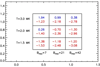
To analyse the role of the background stratified corona we ran a set of nine simulations using three different temperatures (T = 1.5, 2, 3 MK) of the corona and three different maximum

Fig. 1. Grid summarizing the parameter space we investigate. We

ran 9 simulations with all the combinations of T = 1.5, 2, 3 MK withBmax=7, 21, 42 G. The numbers in the cell represent the log10(β)

at the lower boundary (lower number) and the log10(β) at the upper

boundary (higher number). Red are negative values, and blue positive ones.

intensity values of the magnetic field (Bmax =7, 21, 42 G), as illustrated in Fig.1.

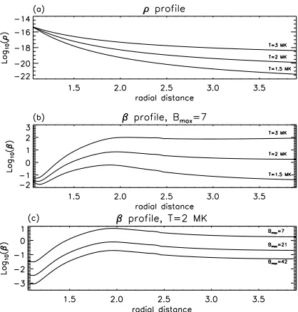
In our model, a higher corona temperature implies a more uniform density and pressure gradient from the photosphere to the outer corona and a higher amount of mass that constitutes the solar corona, as in Fig.2a. At the same time, the higher temper-ature leads to remarkably higherβin the outer corona, as shown in Fig.2b for theBmax = 7 G case, while in the lower corona (r<1.2R)βis clearly below∼10−1regardless of the tempera-ture. For theBmax=21 and 42 G cases, theβvalue is lower. The outer corona switches from a low to a highβregime when the temperature increases from 1.5 to 3 MK (Fig.2b).

We use the temperature to define a part of the parameter space since it is the appropriate parameter to consistently tune the profile of density and thermal pressure in the solar corona. Since we always assume the same value for the photospheric density, an increase in temperature implies a heavier column of mass placed above the magnetic flux rope. By computing the in-tegral of Eq. (7) fromr=1.12Rtor=4R, we get a column of mass of 7.5×10−6g/cm2above the flux rope for the simu-lation withT = 1.5 MK and 25 times more for the simulation withT =3 MK.

At the same time, the pressure scale height reduces when lower temperatures are considered. This implies that the ejected flux rope encounters less resistance from the compression pro-duced ahead when propagating. The pressure length scale is around 0.06R when the temperature is T = 1.5 MK, which doubles to 0.12Rwhen the temperature isT =3 MK. It should be clarified, however, that in our simplified model for the gravi-tational stratification, we do not aim to realistically describe the entire multi-temperature structure of the solar corona, but rather the corona surrounding an active region. In all of the simulations, the density and pressure drop steeply in comparison to the full extent of the computational domain out to 4R.

Simulations with different Bmax (Fig. 2c) basically differ in the plasmaβ, which uniformly decreases as Bmaxincreases. Thus, by changing the parameter Bmax we generally modify the dominant forces and subsequently the capacity of the solar corona to react to the flux rope ejection.

Fig. 2.a)Profiles of log10(ρ) alongrabove the centre of the LHS bipole

for different temperatures of the solar corona,T.b)Profiles of log10(β)

alongrabove the centre of the LHS bipole for different temperatures of the solar corona,T, and withBmax = 7 G.c) Profiles of log10(β)

alongrabove the centre of the LHS bipole with different values of the parameterBmaxand withT =2 MK.

equilibrium profile, but we point out that this can slow down the ejection only slightly, because more plasma has to be displaced as the CME propagates due to the background density (ρbg). However, the kinetic energy carried by the ejected plasma in the flux rope is much greater than the kinetic energy produced by these motions, and these effects can in no way produce ar-tificial ejections. The tests described in the appendix show that such departures from hydrostatic equilibrium only lead to appre-ciable effects on the magnetic configuration on much larger time scales than the one for the CME to escape the solar corona in the present simulations.

3. Results

The initial magnetic field configuration is identical in all of the simulations and it is chosen to produce the ejection of the mag-netic flux rope due to an initial excess of the Lorentz force. Figure3shows the initial magnetic configuration common to all the simulations. The only difference from the one used inPagano et al.(2013) is the larger extension of the domain in the radial di-rection. The flux rope that is about to erupt lies under the arcade system, and external magnetic field lines are shown above. Some of the external magnetic field lines belong to the external arcade. while others are open. A full description of the initial magnetic field configuration is given in Sect. 3.1 ofPagano et al.(2013).

InPagano et al.(2013) the dynamics of the ejection and the production of the initial condition in the GNLFFF simulation is discussed in detail. Here, we only focus on the propagation of the flux rope once the ejection is triggered.

We first describe the characteristics of a typical ejection in this framework. Following this we compare some key features between different simulations in order to highlight the role of the temperature of the stratified corona (T) and the intensity of the magnetic field (Bmax).

Fig. 3.Magnetic field configuration used as the initial condition in all

the MHD simulations. Red lines represent the flux rope, blue lines the arcades, green lines the external magnetic field. The lower boundary is coloured according to the polarity of the magnetic field from blue (negative) to red (positive) in arbitrary units.

Fig. 4.The ejection of the magnetic flux rope. The red lines are all

mag-netic flux rope lines drawn from both the footpoints of the flux rope and from the centre of its axis.

3.1. Typical simulation, (T = 2 MK,Bmax=21 G)

A typical simulation is one withT =2 MK andBmax = 21 G, which is the central one in the parameter space grid shown in Fig.1. In this simulation the flux rope escapes the computational domain at 4Rand a CME occurs. In Fig.4we show the ejection and expansion of the flux rope in 3D to illustrate the simulation with some of the magnetic field lines drawn from the flux rope footpoints and from the axis of the flux rope at different times. In future figures we draw cuts in 2D planes to focus more clearly on specific aspects.

In the initial magnetic configuration (Fig.3), the flux rope lies above the centre of the left-hand side (LHS) bipole, three magnetic arcades connect adjacent and opposite polarities, and a larger arcade connects the opposite external polarities of the two bipoles. The flux rope that is in non-equilibirium lies in the asymmetric part of the global configuration. The density profile falls offwith radial distance whereρ∼10−15g/cm3at the lower boundary andρ ∼ 10−20 g/cm3 _{at the top boundary (Fig.2a).} The plasmaβ is approximately 10−2 near the flux rope and it increases to 10−1radially above it (Fig.2c). We note that there are regions whereβreaches as much as 102_{in the corona (such} as near null points), where the magnetic field is weak.

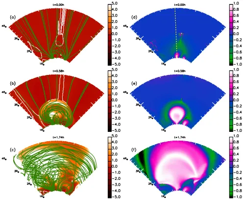
To follow the evolution of the simulation, in Fig.5we show two quantities in ther−φ plane passing through the centre of the bipoles. Figures5a–c show the density contrast,

ρc=ρ(t)_ρ−ρ(t=0)

(t=0) , (10)

Fig. 5.Simulation withT =2 MK andBmax =21 G.a)–c)Maps of

density contrast (Eq. (10)) in the (r−φ) plane passing through the centre of the bipoles att = 0 h,t = 0.58 h,t = 1.74 h. Superimposed are magnetic field lines plotted from the same starting points (green lines) and the contour line ofβ=1 (white line).d)–f)Maps ofB_θ/|B|on the same plane and at the same times. Maps show the full domain of our simulations fromr=1Rtor =4R. In paneld)the yellow dashed line is the cut for the plots in Fig.6. The temporal evolution is available in the on-line edition.

Figures5d–5f show the ratioBθ/|B|that illustrates the evolution of the axial magnetic field of the flux rope, which initially lies in theθ-direction. As explained inMackay & van Ballegooijen (2006), the formation of the flux rope due to magnetic diffusion leads to a strong axial component of the magnetic field along the PIL of the LHS bipole. Simultaneously, the increased tilt of the bipole leads to a quasi-antiparallel magnetic field around the magnetic flux rope. Because of the construction of the system of a E-W bipole and N-S PIL, att =0 the axial magnetic field of the flux rope is mostly along theθdirection and the blue re-gion between pink and green in Figs.5d–f, across whichB_θ/|B|

changes sign, marks the borders of the magnetic flux rope and the overlying arcade. As long as no major reconnection occurs, the quantityB_θ/|B|is clearly positive above the bipoles where the magnetic flux rope propagates and expands.

In this simulation, the flux rope is ejected outwards, and it leads to an increase in density at larger radii (Figs.5a–c), and the propagation and expansion of the region where the mag-netic field is mostly axial, i.e. B_θ/|B| ∼ 1 (Figs. 5c–f). The shape of the density propagation roughly reproduces the typical three-component structure of a CME, which is clearly visible in Fig.5b. A higher density bow front propagates upwards, and be-hind it lies a region with lower density. Finally, a dense core is located at the centre of the expanding dome. In our simulation, the region with highest density coincides with the region where

B_θ/|B|is positive. The quantity B_θ/|B| is maximum just ahead of the high- density region, while the peak of density is highest roughly at the centre of the expanding structure whereB_θ/|B|

remains positive (Fig.5b). This suggests that the magnetic flux rope is propagating upwards, perpendicular to its axial magnetic field lines, lifting coronal plasma to produce the high density re-gion. The same process is seen inPagano et al.(2013), and it is considered a standard process in filament eruptions.

At the same time, the region where a positive axial compo-nent of the magnetic field is dominant expands and propagates

Fig. 6.Profile of B_θ/|B|above the centre of the LHS bipole, at diff

er-ent times (different colours). Dashed lines of different colours indicate whereB_θ/|B|=0 and where we locate the top of the flux rope at a given time.

upwards, roughly covering the same volume of space as that of the high-density region (white and pink region in Figs.5d–f). Since the region whereBθ/|B|>0 roughly reproduces the high-density region that corresponds to the CME, we use this quan-tity to track the ejection and expansion of the CME. Figure6 shows the profile ofB_θ/|B|radially from the centre of the LHS bipole at different times. The radial position where B_θ/|B| =0 along the radial direction vertically from the centre of the LHS bipole is defined to be the top of the magnetic flux rope in our representation.

In the plot in Fig.6we see the top of the flux rope at 1.4R

att = 0 h (black line), and it reaches 3.15Rafter 1.16 h (red line). This clearly shows the ejection of the flux rope.

3.2. Parameter space investigation

3.2.1. Quenched ejections

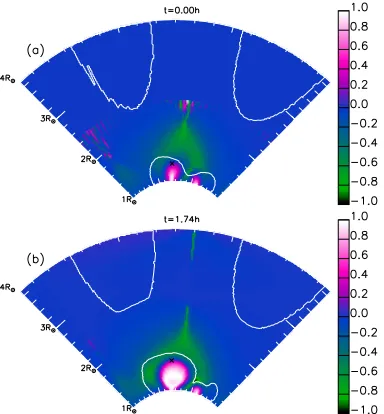
Following the location of the top of the flux rope we are able to track the ejection of the flux rope and thus identify whether the flux rope ejection produces a CME (i.e. extends beyondr = 4 R) or whether it is a quenched ejection. We find that the simulations with T = 2 MK and T = 3 MK whereBmax=7 G do not show any CME propagation. The flux rope only rises up to a given height and then stops. In Fig.7, we show a quenched ejection for the simulation withT =2 MK andBmax = 7 G. In this simulation the magnetic flux rope is stopped and remains positioned atr=1.8Rafter 1.74 h.

A key difference between the simulations where a CME de-velops (Fig. 5a) and where the ejection is quenched (Fig. 7a) is that a high-βregion lies above the flux rope in the simula-tion where the ejecsimula-tion is quenched. The fast CME can only develop in a low-βenvironment. In particular, theβ = 1 con-tour overlies the flux rope in Fig.7a, while it only surrounds the null-point region in Fig.5a. Although this is not a necessary or sufficient condition to determine the onset of a full or quenched ejection, whether a high-βregion lies over the flux rope is one of the factors that can determine the CME evolution.

3.2.2. Parameter space of CMEs

Fig. 7.Simulation withT =2 MK andBmax=7 G. Maps ofBθ/|B|in

the (r−φ) plane passing through the centre of the bipoles att= 0 h andt=1.74 h. Superimposed is the contour line ofβ=1 (white line). Black crosses indicate where the top of the flux rope is positioned.

the top of the flux rope as soon as it is close to the outer boundary and its propagation is affected by boundary effects. The speed quoted in Fig.8 is the average speed of propagation. The av-erage speed of the CME spans a wide range from 69 km s−1 to 498 km s−1. The lower the temperature, the faster the CME. Also, the CMEs propagating in a 2 MK or 1.5 MK corona are at near constant speed, while the speed varies slightly with radial distance for the slowest CME (T =3 MK).

Figure 8b shows the height of the top of the flux rope as a function of time for the three simulations with T = 2 MK (central row in Fig.1). The higher the magnetic field (Bmax), the stronger the initial force due to the unbalanced Lorentz force under the magnetic flux rope, and the CME travels faster. WithBmax =7 G, we have a quenched ejection, while we have a 718 km s−1fast CME withBmax=42 G. By changing the pa-rameter Bmax, we change the Alfvén speed in the system and thus the evolution time scale. It should be noted that the re-sult of the simulations with different Bmax cannot be inferred solely through timescale arguments owing to the presence of the plasma. For instance, this is demonstrated by the qualitatively different evolution of the simulation withBmax =7 G from the other simulations.

We note that the speed of the top of the flux rope is not neces-sarily the speed of the CME. The top of the flux rope represents the leading edge of the CME, which is subjected to the com-bined effect of propagation and expansion. However, the results approximately indicate the speed of the CME and its dependence on the parametersT andBmax. In Fig.9we summarize the speed of the CMEs for all of the simulations. The fastest CME in our simulations can reproduce speeds of 838 km s−1, and only two simulations show a quenched ejection.

We also use the quantityB_θ/|B|to follow theφextension of the flux rope and thus its expansion. We draw the contour of the flux rope by tracking where the cut ofB_θ/|B|along theφ direc-tion on ther-φplane passing through the centre of the bipoles changes sign at different radial distances. Then, we consider the maximum φ extension of the resulting flux rope contour. Figure10a shows the extension of the flux rope as a function of the height of the top of the flux rope for the simulations where

Fig. 8.a)Position of the top of the flux rope as a function of time in the

three simulations withBmax =21 G.b)Position of the top of the flux

rope as function of time in the three simulations withT =2 MK.

Fig. 9.Grid summarizing the average speed of the CME in the

param-eter space we investigate. Crosses indicate a quenched ejection, and in the other boxes we write the value of the CME speed computed from tracking the top of the flux rope as in Fig.8.

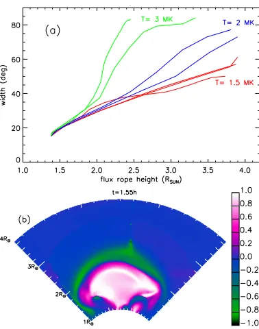
unquenched eruptions occur. In this plot we group the simula-tions by temperature with different colours. The intensity of the magnetic fieldBmax does not significantly influence the expan-sion of the CME, i.e. its shape. This can be seen because lines with the same colour lie close to one another in Fig.10a. In con-trast, the background temperature,T, plays a significant role in shaping the ejection.

Fig. 10.a)Angular extension of the flux rope as a function of the radial distance of the top of the flux rope for all the simulations that show a CME. Simulations are grouped according to the simulation parameterT

given with different colours.b)Map ofB_θ/|B|in the (r−φ) plane pass-ing through the centre of the bipoles att = 1.55 h for the simulation withT =3 MK andBmax =21 G. The map shows the full domain of

our simulations fromr=1Rtor=4R.

withT =3 MK show an expansion that is about twice as large as the expansion found in the simulations with a cooler stratified solar corona.

In summary, Fig.10a shows that higher temperatures favour higher expansion of the CME, which in turn results in a flattened shape. The higher pressure and density above the ejecting flux rope slow down the radial propagation and favour the expansion of the CME towards the sides. An example of the different shape of the CME is given in Fig.10b where we show a snapshot of the simulation withT =3 MK andBmax=21 G (to be compared with Fig.5e).

4. Discussion

In this paper we have considered the role of gravitational strati-fication on the propagation of a CME. In order to do so, we in-vestigated the parameter space by tuning the temperature of the corona (i.e. gravity stratification) and the maximum value of the magnetic field (i.e. the entireβof the corona). The techniques and the initial magnetic configurations are identical to those of Pagano et al.(2013) where a CME initiation was successfully modelled.

4.1. Comparison with the flux rope ejection simulated in Pagano et al. (2013)

The purpose of the present work is not to analyse the mechanism that initiates the flux rope ejection in detail, since it does not show any significant difference from what is described inPagano et al.(2013). However, once the onset of the ejection occurs, some differences appear in the CME propagation depending on the characteristics of the background corona, and in the present

paper we try to get some physical insight into the underlying physics involved. In contrast to the background coronal model inPagano et al. (2013), the plasma pressure and density pro-file in the present simulations are a consequence of gravitational stratification.

A drop in thermal pressure implies that the ejection encoun-ters less resistance from the solar corona, which should aid the production of a CME. While this is true, it should be noted that the ejected plasma is now subject to the gravity force that was not considered previously. The two effects nearly balance out since the speed of the ejection is generally comparable to the ones measured inPagano et al.(2013). It should be noted, how-ever, that slightly higher speeds are obtained in the present work. Another aspect is that because of the lower thermal pressure in the outer solar corona, the interaction between the ejected flux rope and the surrounding plasma is reduced, and this leads to a clearer three-component structure of the CME. Our present sim-ulations clearly show the light-bulb structure that was not seen in Pagano et al.(2013). For the same reason, significantly less mag-netic reconnection due to numerical diffusion occurs between the flux rope magnetic field and the external arcade magnetic field, resulting in higher coherence of the expelled flux rope and less mixing between the flux-rope magnetic field lines and the external arcade magnetic field lines.

4.2. Role of plasmaβon CME speed

In this study, the plasmaβplays a major role in determining the evolution of the system. Firstly, the plasmaβdistribution deter-mines whether an ejection is quenched or if it will escape the solar corona. In simulations where only lowβplasma covers the initial flux rope, it quickly reaches a height of 4R. In contrast to the two simulations (Fig.9) where the ejection stops, the flux rope is surrounded by highβplasma (see Fig.7a). In our study we have used coronal values for magnetic field intensity, density of plasma, and temperature, and our simulations seem to confirm that the onset of solar eruptions is caused by a purely magnetic process, but the evolution of a flux rope ejection does depend on the plasma parameters. This is an important factor to be con-sidered when we wish to address the issue of CME generation, especially in the space weather context.

Secondly, a lower plasma β seems to favour higher CME speed. In our investigation of the parameter space this was done by increasing the intensity of the flux rope magnetic field by a factor of 3 or 6. Such an increase leads to an increase of a fac-tor of 5 or 8 in the CME speed (simulations withT =1.5 MK in Fig.9). Similar results are found when comparing the CME speed in the ejecting simulations atT =2 MK andT =3 MK,

4.3. Role of gravitational stratification on CME speed

In the framework of the present study, another way of tuning the plasmaβin the outer corona is to change the coronal tem-perature. In particular, the colder the atmosphere, the lower the plasmaβ, and the more likely a full ejection occurs. However, tuning the temperature only affects the capacity of the outer corona to react to the ejection, but not the initial force to which the flux rope is subject. For this reason, in our framework the temperature of the corona has a weaker effect compared to the magnetic field intensity in producing CMEs at higher speeds. At the same time, the role of the temperature stratification de-serves more detailed analysis in future studies. In fact, it is re-markable that simulations where the coronal temperature only differs by 0.5 MK show such a different behaviour. This could be the reason for the enhancement of some CMEs in the solar corona. Similar to the work ofLin(2004), we find that the gravi-tational force can be effective on the flux rope ejection when the magnetic field is relatively weak. In particular, it can only slow down the ejected flux rope when the magnetic field is relatively weak. In future, we need to investigate the cause of the flux rope ejections more. In our study, the ejection is caused by the build up of an excess of the Lorentz force; however, the question re-mains open whether a MHD instability, like the Torus instability (Kliem & Török 2006), could explain the ejection. In our case, a treatment like the one ofKliem & Török(2006) should include the role of thermal pressure and gravity. In doing so, the critical index for the enhancement of the ejection could be determined as could whether it differs from previous studies.

4.4. Role of gravity stratification on CME expansion

Another result of our study is that the gravitational stratifica-tion can be responsible for shaping the CME, since the thermal pressure ahead of the CME front can stimulate an expansion at its sides. We identified this effect in particular in the simulation withT =3 MK andBmax=21 G where the expanding CME ac-quires a shape that is significantly different from the ones found in other simulations. However, the result is more general, as shown in Fig.10b. From the analysis of our simulations, we find that the width of the CME bulb can be significantly different from one simulation to the next if different coronal temperatures are considered.

Further studies are required, but in principle different strati-fications may be responsible for the variety of CME shapes ob-served. In particular, the CME we describe in the simulation withT = 3 MK and Bmax = 21 G seems to be very similar to the ejection that occurred on June 13, 2010 as described by Gopalswamy et al.(2012). It is remarkable how the CME shape in our simulation matches the snapshot of the ejection at 5:40:54, where not only is the front profile reproduced, but the northern side of the ejection also seems to behave as if there is another bipole besides the one involved in the ejection as in our simula-tion (Fig.10b). It should, however, be noted that inGopalswamy et al.(2012) the CME is observed at 1.4R, significantly lower than our snapshot in Fig.10b. Also Patsourakos et al. (2010) studied the expansion of a CME and found the expansion to be initially very rapid and characterized by a self-similar evolution at later times. Our results differ from their findings, since in our simulations the CME bubble expansion agrees with a constant decrease in the aspect ratio (radial position/radius), and it never reaches the self-similar regime. Such a difference in our results could be explained by the lack of an outflowing solar wind in our simulations that would contribute to narrowing the propagation of the CME. This feature will be investigated in future studies.

5. Conclusions

The present study aims at understanding the role of gravitational stratification in the propagation of CMEs. To identify the role of gravitational stratification, we ran several simulations that vary two quantities: the stratification temperature (T) and plasmaβ. In all simulations an identical magnetic field configuration is used that has been proven to be suitable for an ejection.

Our work appeared to produce a reasonable model for the early evolution of actual CMEs, since observations show that the CME acceleration tends to vanish above 4 R (Vršnak 2001), when the CME kinematics couple to the solar wind (Gopalswamy et al. 2000). Therefore our model covers the do-main of initiation of a CME, and we can reasonably assume that all the ejections that leave our domain would not need any further acceleration mechanisms to travel through interplanetary space dragged by the solar wind.

This study showed that gravitational stratification has an im-portant effect on the propagation of CMEs in the solar corona through the way it specifies how large the plasmaβbecomes. We also find that the plasmaβdistribution is a crucial parame-ter that deparame-termines whether a flux rope ejection escapes the solar corona, turning into a CME, or if it just makes the flux rope find a new equilibrium at a greater height. Similarly, we find that a cooler solar corona (T ∼ 1.5 MK) can help the escape of the CME and make it travel faster.

Both of these results – first the importance of a low β region above the magnetic flux rope to allow the ejection and secondly the role of the coronal temperature in the CME speed – can be tested with observations where 3D magnetic field reconstructions are carried along with simultaneous den-sity and temperature diagnostics to infer the plasma stratifica-tion. However, magnetic field reconstructions are more reliable from disk observations, which makes it very difficult to infer coronal stratification because of line-of-sight integration effects. However, future missions of the STEREO type with this capacity could be required.

Acknowledgements. The authors would like to thank Dr. Bernhard Kliem for useful discussions and suggestions. The authors would also like to thank the referee for the constructive and positive feedback on the manuscript. D.H.M. would like to thank STFC, the Leverhulme Trust and the European Commission’s Seventh Framework Programme (FP7/2007-2013) for their financial support. P.P. would like to thank the European Commission’s Seventh Framework Programme (FP7/2007-2013) under grant agreement SWIFF (project 263340,http://www.swiff.eu) for financial support. These results were obtained in the framework of the projects GOA/2009-009 (KU Leuven), G.0729.11 (FWO-Vlaanderen), and C 90347 (ESA Prodex 9). The research leading to these results has also received funding from the European Commission’s Seventh Framework Programme (FP7/2007-2013) un-der the grant agreements SOLSPANET (project No. 269299, http://www. solspanet.eu), SPACECAST (project No. 262468, fp7-spacecast.eu), and eHeroes (project No. 284461,http://www.eheroes.eu). The computational work for this paper was carried out on the joint STFC and SFC (SRIF) funded cluster at the University of St Andrews (Scotland, UK).

Appendix A: Equilibrium tests

Fig. A.1.Maps of log10(ρ[g/cm3]) in the (r−φ) plane passing through

the centre of the bipoles at different times for different test simulations. Superimposed are magnetic field lines plotted from the same starting points (green lines) and the contour line ofβ=1 (white line).a)and d)T =3 MK,Bmax =7 G;b)ande)T =2 MK,Bmax=21 G;c)and

f)T =1.5 MK,Bmax=42 G.

This test is performed using an initial force-free magnetic condition similar to the case we wish to investigate, consisting of two magnetic bipoles that lie close to one another but do not overlap. We refer toPagano et al.(2013) for further details on the magnetic configuration.

We consider several stratified density and pressure profiles that cover the parameter space described in Sect.2.2. Namely, we show here in Fig.A.1simulations with (T =3 MK,Bmax= 7 G), (T = 2 MK, Bmax = 21 G), and (T = 1.5 MK, Bmax = 42 G).

To test the stability, we let the system evolve for a large num-ber of Alfvén times. In the simulation with Bmax = 7 G, we estimate the Alfvén timeτAlf = 120 s as the time it takes an Alfvén wave to travel across a single bipole with a typical speed of 800 km s−1. Consequently, the Alfvén time is τAlf = 40 s andτAlf =20 s for the simulations withBmax=21 G andBmax= 42 G. FigureA.1shows the density contrast (defined in Eq. (10)). The plasma density contrast does not show any significant evo-lution for any of the test simulations, even though small-scale changes occur.

The only test that shows an observable change in the mag-netic structure is the one withT =1.5 MK andBmax =42 G. This is due to the non-zero values of pbg andρbg that lead to a downward bulk motion of plasma in the higher part of the corona, as explained in Sect. 2.2. After this occurs, numeri-cal reconnection takes place, and some of the initially open magnetic field lines reconnect near the outer boundary. However,

only a small change in the magnetic configuration can be seen after∼3.3 h, equivalent in this particular simulation to 600τalf. In the corresponding simulation in Sect.3.2where a CME oc-curs, the magnetic flux rope reaches the top of the domain in less than 0.8 h. Therefore the motions due to the non-zero val-ues ofpbgandρbgare negligible in comparison to the dynamics produced by the flux rope ejection.

These tests show that the transporting between the GNLFFF and MHD models is possible when including the effects of grav-ity, a stratified atmosphere, and magnetic field intensity tuning and that these changes do not generate numerical artefacts in the MHD simulation.

References

Amari, T., Luciani, J. F., Mikic, Z., & Linker, J. 2000, ApJ, 529, L49

Antonucci, E., Dodero, M. A., Giordano, S., Krishnakumar, V., & Noci, G. 2004, A&A, 416, 749

Archontis, V., Hood, A. W., Savcheva, A., Golub, L., & Deluca, E. 2009, ApJ, 691, 1276

Bemporad, A., Mierla, M., & Tripathi, D. 2011, A&A, 531, A147 Chen, J. & Krall, J. 2003, J. Geophys. Res., 108, 1410

Ciaravella, A., Raymond, J. C., Reale, F., Strachan, L., & Peres, G. 2001, ApJ, 557, 351

Fan, Y., & Gibson, S. E. 2007, ApJ, 668, 1232 Forbes, T. G., & Isenberg, P. A. 1991, ApJ, 373, 294 Gary, G. A. 2001, Sol. Phys., 203, 71

Gopalswamy, N. 2004, in The Sun and the Heliosphere as an Integrated System, eds. G. Poletto, & S. T. Suess, ASSL, 317, 201

Gopalswamy, N., Lara, A., Lepping, R. P., et al. 2000, Geophys. Res. Lett., 27, 145

Gopalswamy, N., Nitta, N., Akiyama, S., Mäkelä, P., & Yashiro, S. 2012, ApJ, 744, 72

Guhathakurta, M., Fludra, A., Gibson, S. E., Biesecker, D., & Fisher, R. 1999, J. Geophys. Res., 104, 9801

Hundhausen, A. J. 1987, in Sixth International Solar Wind Conference, eds. V. J. Pizzo, T. Holzer, & D. G. Sime, 181

Innes, D. E., Cameron, R. H., Fletcher, L., Inhester, B., & Solanki, S. K. 2012, A&A, 540, L10

Keppens, R., Meliani, Z., van Marle, A. J., et al. 2012, J. Comput. Phys., 231, 718

Kliem, B., & Török, T. 2006, Phys. Rev. Lett., 96, 255002

Lee, J.-Y., Raymond, J. C., Ko, Y.-K., & Kim, K.-S. 2009, ApJ, 692, 1271 Lin, J. 2004, Sol. Phys., 219, 169

Mackay, D. H., & van Ballegooijen, A. A. 2006, ApJ, 641, 577

Manchester, W. B., Gombosi, T. I., Roussev, I., et al. 2004, J. Geophys. Res., 109, 2107

Pagano, P., Reale, F., Orlando, S., & Peres, G. 2007, A&A, 464, 753 Pagano, P., Mackay, D. H., & Poedts, S. 2013, A&A, 554, A77 Patsourakos, S., Vourlidas, A., & Kliem, B. 2010, A&A, 522, A100 Pomoell, J., & Vainio, R. 2012, ApJ, 745, 151

Powell, K. G., Roe, P. L., Linde, T. J., Gombosi, T. I., & de Zeeuw, D. L. 1999, J. Comput. Phys., 154, 284

Reeves, K. K., Linker, J. A., Miki´c, Z., & Forbes, T. G. 2010, ApJ, 721, 1547 Roussev, I. I., Galsgaard, K., Downs, C., et al. 2012, Nat. Phys., 8, 845 Temmer, M., Vršnak, B., Rollett, T., et al. 2012, ApJ, 749, 57 Verma, A. K., Fienga, A., Laskar, J., et al. 2013, A&A, 550, A124 Vršnak, B. 2001, J. Geophys. Res., 106, 25249

Zhang, J., Dere, K. P., Howard, R. A., Kundu, M. R., & White, S. M. 2001, ApJ, 559, 452