Galaxy And Mass Assembly (GAMA) : the sSFR M* relation part I σsSFR M* as a function of sample, SFR indicator, and environment

Galaxy And Mass Assembly (GAMA): The sSFR–M

_∗

relation part I –

σ

sSFR

–M

∗

as a function of sample, SFR indicator, and environment

L. J. M. Davies ,

C. del P. Lagos ,

A. Katsianis ,

A. S. G. Robotham ,

L. Cortese ,

S. P. Driver,

M. N. Bremer,

M. J. I. Brown,

S. Brough ,

M. E. Cluver ,

M. W. Grootes,

B. W. Holwerda ,

M. Owers

and S. Phillipps

1_{ICRAR, The University of Western Australia, 35 Stirling Highway, Crawley, WA 6009, Australia} 2_{ARC Centre of Excellence for All Sky Astrophysics in 3 Dimensions (ASTRO 3D)}

3_{Department of Astronomy, Universitad de Chile, Camino El Observatorio 1515, Las Condes, 7591245 Santiago, Chile} 4_{School of Physics, University of Bristol, Tyndall Avenue, Bristol BS8 1TL, UK}

5_{School of Physics and Astronomy, Monash University, Clayton, VIC 3800, Australia} 6_{School of Physics, University of New South Wales, Sydney, NSW 2052, Australia}

7_{Centre for Astrophysics and Supercomputing, Swinburne University of Technology, John Street, Hawthorn, VIC 3122, Australia} 8_{Department of Physics and Astronomy, University of the Western Cape, Robert Sobukwe Road, Bellville 7535, South Africa} 9_{ESA/ESTEC SCI-S, Keplerlaan 1, NL-2201 AZ Noordwijk, the Netherlands}

10_{Department of Physics and Astronomy, University of Louisville, 102 Natural Science Building, Louisville, KY 40292, USA} 11_{Department of Physics and Astronomy, Macquarie University, North Ryde, NSW 2109, Australia}

Accepted 2018 October 29. Received 2018 October 28; in original form 2018 September 6

A B S T R A C T

Recently, a number of studies have proposed that the dispersion along the star formation rate (SFR) – stellar mass relation (σsSFR–M∗) – is indicative of variations in star formation history

driven by feedback processes. They found a ‘U’-shaped dispersion and attribute the increased scatter at low and high stellar masses to stellar and active galactic nuclei feedback, respectively. However, measuringσsSFRand the shape of theσsSFR–M∗relation is problematic and can vary

dramatically depending on the sample selected, chosen separation of passive/star-forming systems, and method of deriving SFRs (i.e. Hαemission versus spectral energy distribution fitting). As such, any astrophysical conclusions drawn from measurements of σsSFR must

consider these dependencies. Here, we use the Galaxy And Mass Assembly survey to explore howσsSFRvaries with SFR indicator for a variety of selections for disc-like ‘main-sequence’

star-forming galaxies including colour, SFR, visual morphology, bulge-to-total mass ratio, S´ersic index, and mixture modelling. We find that irrespective of sample selection and/or SFR indicator, the dispersion along the sSFR–M_∗ relation does follow a ‘U’-shaped distribution. This suggests that the shape is physical and not an artefact of sample selection or method. We then compare theσ_sSFR–M_∗relation to state-of-the-art hydrodynamical and semi-analytic models and find good agreement with our observed results. Finally, we find that for group satellites this ‘U’-shaped distribution is not observed due to additional high scatter population at intermediate stellar masses.

Key words: galaxies: evolution – galaxies: general – galaxies: groups: general.

1 I N T R O D U C T I O N

Star-forming galaxies over a range of epochs and environments have been found to display a tight correlation between their star formation

rate (SFR) and stellar mass (M_∗), described as the star-forming

sequence (SFS, or star-forming ‘main sequence’; Elbaz et al.2007;

Noeske et al.2007; Salim et al.2007; Whitaker et al.2012; Davies

_{E-mail:[email protected]}

et al.2016). This sequence has been shown to be largely linear out

to high redshift, but with increasing normalization as a function

of look-back time (e.g. Lee et al.2015; Schreiber et al.2015). The

physical interpretation of these observations (i.e. Bouch´e et al.2010;

Daddi et al.2010; Genzel et al.2010; Lagos et al.2011; Dav´e et al.

2013; Lilly et al.2013; Mitchell et al.2016) is that the bulk of

star-forming galaxies reside in a self-regulated equilibrium state, where the inflow rate of gas for future star formation is balanced by the rate at which new stars are formed and the outflow of gas from feedback events [i.e. supernovae (SNe) and active galactic nuclei (AGN)].

2018 The Author(s)

However, within the full sSFR–M∗ plane the situation is more complex. While this simple self-regulated model is likely to fit for sources that sit close to the locus of the SFS, there exist various other population that deviate from this model, such as the passive cloud that sits below the SFS, ‘green valley’ sources that sit be-tween the SFS and passive cloud, and star-bursting sources that reside above the SFS. More recent results have found that galaxies move significantly within the SFS over their lifetime based on small

star-burst/quenching events (i.e. Magdis et al.2012; Tacchella et al.

2016), such that the locus of the SFS remains constant at a given

epoch, but with individual galaxies move within the SFS producing the observed scatter. In addition, there has been recent evidence to suggest that the SFS is non-linear in the high stellar mass regime

and flattens (e.g. Rodighiero et al.2010; Elbaz et al.2011; Whitaker

et al.2012; Lee et al. 2015; Katsianis, Tescari & Wyithe2016;

Grootes et al.2017,2018). This is likely to be caused by the

inclu-sion of non-star-forming bulge components in stellar mass estimates

at log10[M∗/M]>10 (Erfanianfar et al.2016). The flattening is

found to be removed when only considering disc-dominated

sys-tems (e.g. Abramson et al.2014; Willett et al.2015) and/or just the

disc components of galaxies (Davies et al., in preparation – paper II in this series – and Cook et al., in preparation).

The position of a galaxy within the sSFR–M_∗plane is largely

determined by its star formation history (SFH, Madau, Pozzetti &

Dickinson1998; Kauffmann et al.2003). This history is governed

by many events, which occur in the lifetime of the galaxy that

can fundamentally affect its trajectory through the sSFR–M_∗plane,

such as gas accretion (Kauffmann et al.2006; Sancisi et al.2008;

Mitchell et al.2016), mergers (e.g. Bundy et al.2004; Baugh2006;

Kartaltepe et al.2007; Bundy et al.2009; de Ravel et al.2009; Jogee

et al.2009; Lotz et al.2011; Robotham et al.2014, and see review

of Conselice2014), SNe feedback (Dekel & Silk1986; Dalla

Vec-chia & Schaye2008; Scannapieco et al.2008), and AGN feedback

(Kauffmann et al.2004; Fabian2012), environmental effects such as

starvation, strangulation, and stripping (e.g. Giovanelli & Haynes

1985; Moore et al.1999; Peng et al. 2010; Cortese et al.2011;

Darvish et al.2016), and morphological changes (Conselice2014;

Eales et al.2015). It is the combination of these SFHs that ultimately

result in the distribution of points in the sSFR–M_∗plane

(Abram-son et al.2016). As such, understanding the global distribution of

sources within this plane, the position of various sub-population split on properties such as environment, morphology and structure, and physical mechanisms that result in galaxies moving through the plane is essential to our parametrization of the factors driving galaxy evolution.

One key diagnostic of these physical mechanisms is the

disper-sion along the sSFR–M∗relation (σsSFR–M∗, Guo et al.2015; Willett

et al.2015; Katsianis et al., in preparation). This dispersion is

es-sentially a metric of the variation in a galaxy’s recent SFH at a given stellar mass. For example, recent quenching and star-burst events push galaxies below and above the SFS, respectively, increasing the dispersion. In addition, as these events have opposite effects in terms of sSFR, asymmetry in the distribution of points about the SFS at a given mass is indicative of predominant quenching/starbursts

There is currently rich debate as to the shape of theσsSFR–M∗

relation. At high redshifts (z > 1) and for predominantly

UV-derived SFRs, authors have generally found a relatively constant

dispersion of∼0.3 dex (Elbaz et al. 2007; Noeske et al. 2007;

Rodighiero et al.2010; Whitaker et al.2012; Schreiber et al.2015).

However, other authors have suggested that this dispersion may

increase with decreasing stellar mass at log10[M∗/M] < 10 in

high-redshift samples and be driven by stochastic SFHs in

low-mass galaxies (Santini et al.2017). For more nearby samples and

higher stellar mass galaxies, other studies have identified a

disper-sion that increases at log10[M∗/M]> 10 (Guo et al.2015) and

attribute the large dispersion to the presence of bulges and bars (their sample is purely selected based on sSFR and thus contain

bulge+disc systems). To overcome this, Willett et al. (2015)

ex-plore theσsSFR–M∗relation in a morphologically selected sample

of disc-like spirals from Galaxy Zoo (Willett et al.2013). They

find a minimum vertex parabolic (‘U’-shaped) dispersion that

de-creases with stellar mass from log10[M∗/M] ∼ 8–10 and then

increases at log10[M∗/M] ∼ 10–11.5. This is loosely

consis-tent with the Guo et al. (2015) results at the high-mass end, but

finds the upturn in dispersion occurs at higher masses. In addition, there also appears to be some variation in the literature

measure-ments ofσsSFR–M∗depending on the SFR indicator used; with UV-,

Hα-, and SED-derived SFRs producing different dispersions. This

is potentially due to the varying biases included in different SFR indicators and the physical time-scales over which they probe;

for example Hα-derived SFRs are much more sensitive to short

time-scale fluctuations in SFH (for a detailed discussion of SFR indicators, their biases, and time-scales see Kennicutt & Evans

2012; Davies et al.2015b, 2016, and Katsianis et al.2017for a

simulations perspective).

Evidently the observational picture is far from clear, with differ-ent teams applying differdiffer-ent selection methods and using differdiffer-ent SFR indicators finding different results. However, hydrodynamical

simulations can offer some further insights into theσsSFR–M∗

rela-tion and the physical processes driving its shape. Sparre et al. (2015)

use the Illustris simulation (Vogelsberger et al.2014) to explore the

evolution of the sSFR–M_∗relation for all Illustris galaxies and atz

∼0 find a relatively flatσsSFR–M∗at 9<log10[M∗/M]<10.5 and

increasing dispersion to higher masses. However, they do not make any selection to exclude passive systems, and hence this increased dispersion is likely due to the passive population becoming more prevalent at high stellar masses.

More recently, Katsianis et al. (in preparation) applied a similar

approach to the EAGLE simulation (Crain et al.2015; Schaye et al.

2015; McAlpine et al.2016; Matthee & Schaye2018) and find a

minimum vertex parabolic (‘U’-shaped)σsSFR–M∗relation similar

to that of Willett et al. (2015) – note that Matthee & Schaye (2018)

find a linearly decreasing σsSFR–M∗when excluding the passive

population based on sSFR (which we also explore here). Moreover, the work of Katsianis et al. (in preparation) also allows an explo-ration of the physical mechanisms that are driving this dispersion. First, they rerun their analysis with no-AGN feedback and find that the dispersion is dramatically reduced at the high stellar mass end, suggesting it is AGN feedback that drives the high dispersion at

log10[M∗/M]∼10–11.5 observed by Guo et al. (2015) and

Wil-lett et al. (2015) – this is also discussed in Matthee & Schaye (2018).

Next, they rerun their analysis with stellar feedback turned off and find a reduced scatter at the low stellar mass end, suggesting it is stellar feedback/star formation that drives the observed dispersion at these lower masses.

Similarly, using the semi-analytic model (SAM), Shark, Lagos

et al. (2018) showed that the adopted star formation law had a

strong effect on the scatter of the SFS (through their effect on the time-scales of atomic to molecular hydrogen and molecular-to-stars conversion). However, the choice of star formation law rarely affected the zero-point of the main sequence. These simulation results suggest that the scatter of the SFS is rich in information about the physics of galaxy formation and provide us with both a

prediction for the shape of theσsSFR–M∗relation and the physical

mechanisms driving it. We must now aim to test this prediction via our observational samples.

In this series of papers, we produce a detailed analysis of the

sSFR–M_∗plane and the factors driving its formation. In this first

paper, we explore the observed dispersion along the SFS and its variation with sample selection, SFR indicator, and group/isolated environment using the Galaxy And Mass Assembly (GAMA)

sam-ple. We explore whether the variation in thez∼0σsSFR–M∗

ob-served by previous authors is physical or an artefact of their chosen

method. Following this, we will determine how the sSFR–M∗plane

can be sub-divided into different population based on various mor-phological and structural tracers, how this varies with environment, and how these population are indicative of different evolutionary

pathways through the sSFR–M_∗plane. Finally, we will use our new

SED fitting codePROSPECT(Robotham et al., in preparation) to

de-termine SFHs and AGN fractions for galaxies across the sSFR–M_∗

plane and explore the physical mechanisms that have shaped thez

∼0 SFR–M_∗relation using all observations presented in the series.

This paper is organized as follows. In Section 2, we discuss the ob-servational samples used in this work and briefly describe our choice of SFR indicators. In Section 3, we detail different methods for se-lecting the SFS based on SFR, colour, and morphology/structure.

In Section 4, we present the resultantσsSFR–M∗ relation derived

from each sample and explore its variation with SFR indicator and environment. We also compare our results to the Shark and EA-GLE simulations. Finally, in Section 5 we present our conclusions.

Throughout this paper, we use a standardCDM cosmology with

H0 = 70 km s−1Mpc−1, = 0.7, andM = 0.3.

2 DATA A N D S A M P L E S E L E C T I O N S

2.1 Galaxy And Mass Assembly Survey

The GAMA survey covers 286 deg2 _{to a main survey limit of}

rAB<19.8 mag in three equatorial (G09, G12, and G15) and two

southern (G02 and G23 survey limit ofiAB < 19.2 mag in G23)

regions. The limiting magnitude of GAMA was initially designed to probe all aspects of cosmic structures on 1 kpc to 1 Mpc scales

spanning all environments and out to a redshift limit ofz∼0.4.

The spectroscopic survey was undertaken using the AAOmega

fibre-fed spectrograph (Saunders et al.2004; Sharp et al.2006) in

conjunction with the two-degree field (Lewis et al.2002) positioner

on the Anglo–Australian telescope and obtained redshifts for

∼240 000 targets covering 0< z0.5 with a median redshift ofz

∼0.25, and highly uniform spatial completeness (see Baldry et al.

2010; Robotham et al.2010; Driver et al. 2011; Hopkins et al.

2013, for summary of GAMA observations).

Full details of the GAMA survey can be found in Driver et al.

(2011,2016a), Liske et al. (2015), and Baldry et al. (2018). In this

work, we utilize the data obtained in the three equatorial regions,

which we refer to here as GAMA IIEq. Stellar masses for the GAMA

IIEq sample, and those used in this work, are derived from the

ugriZYJHKphotometry using a method similar to that outlined in

Taylor et al. (2011) – assuming a Chabrier initial mass function

(IMF; Chabrier2003), GAMA DMU StellarMassesLambdarV20.

All photometry used in this work is measured using the Lambda Adaptive Multi-Band Deblending Algorithm for R and presented in

Wright et al. (2016), GAMA DMU LambdarPhotometryV01.

In this paper, we also use the recent GalaxyZoo classifications that are based on the Kilo Degree Survey (KiDS, de Jong et al.

2013,2015,2017) imaging in the GAMA regions. For these

classi-fications, 49 851 galaxies were selected from the GAMA equatorial

0 0.05 0.1 0.15

10

7

10

8

10

9

10

10

10

11

10

12

Redshift

Stellar

Mass,

Mʘ

GAMA Galaxies Sample used in this paper

0.8 0.9 1 1.1 1.2 1.3 1.4 1.5

u

*-r

*

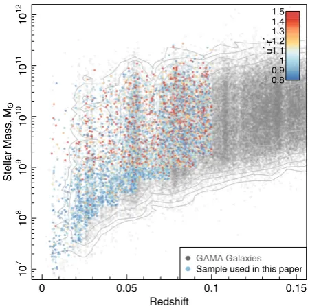
Figure 1. The redshift–stellar mass distribution of galaxies used in this work in comparison to the full GAMA sample. We initially se-lect isolated (non-group or pair) galaxies in volume-limited samples in log10[M∗/M]=0.25 bins of stellar mass (see Section 2.1 for details).

Selected points are coloured by their rest-frame, extinction-correctedu−r colour. The contours display the density of GAMA points.

fields with redshiftsz <0.15. Within GalaxyZoo, the GAMA

sam-ple received almost two million classifications from over 20 000 unique users in 12 months. The GAMA–KiDS GalaxyZoo clas-sifications use the standard decision tree implemented for cur-rent GalaxyZoo projects. A full description of the GAMA–KiDS GalaxyZoo effort can be found in Kelvin et al. (in preparation).

In this work, we further restrict our sample to galaxies within rolling volume-limited samples and initially galaxies that are not in either a group or pair in the GAMA group catalogues of Robotham

et al. (2011), i.e. isolated centrals, GAMA DMU GroupFindingV10.

To define our volume-limited samples, we follow a similar

ap-proach to Lange et al. (2016) and split the full GAMA catalogue

intolog10[M∗/M] =0.25 bins of stellar mass. For each bin,

we calculate the redshift where 97.7 per cent of the sample has a

maximum observable redshift (Vmax) greater than the medianVmax

of the bin. We then exclude all galaxies above this redshift, within the particular stellar mass bin. Finally, we put an upper redshift limit ofz <0.1. This process allows us to extend to lower stellar masses in our very local sample.

The resultant redshift–stellar mass selection of our sample in

comparison to the full GAMA sample is shown in Fig.1. Thez <

0.1 restriction is to largely remove any evolution in the SFS across our sample redshift range. In addition, a number of GAMA data

products that are required for our analysis are only available forz <

0.1 GAMA galaxies (see Section 3). The isolated centrals restriction allows us to remove any additional environmental quenching effects that may induce additional scatter in the SFS, which is not driven

by feedback (however, c.f. Barsanti et al.2018, find that groups can

affect galaxies SF properties out to large radii). Note that we do not include group centrals in our sample as there is currently some debate as to whether or not these galaxies undergo environmental

quenching (e.g. see Wang et al.2018). However, we do perform our

analysis including group centrals and find that it does not

cantly affect our results. The effect of group environment onσsSFR

is then explored further in Section 4.3 and in the following papers in this series. In total, there are 9005 galaxies in our starting sample.

2.1.1 GAMA SFR indicators

The GAMA SFR indicators used in this work are described at length

in Davies et al. (2016). Briefly, we use (i)MAGPHYS-derived SFRs

outlined in Driver et al. (2018) and based on the energy balance

SED-fitting codeMAGPHYS(da Cunha, Charlot & Elbaz2008), (ii)

combined Ultraviolet and Total Infrared (UV+TIR) SFRs derived

from the Brown et al. (2014) galaxy spectra, (iii) Hα-derived SFRs

using GAMA spectra discussed in Liske et al. (2015) and the

pro-cess outlined in Gunawardhana et al. (2011, 2015) and Hopkins

et al. (2013), and using the line measurements of Gordon et al.

(2017), (iv)Wide-field Infrared Survey Explorer(WISE) W3-band

SFRs derived using the prescription outlined in Cluver et al. (2017),

and (v) extinction-correctedu-band SFRs derived using the GAMA

rest-frameu-band luminosity andu−gcolours from Davies et al.

(2016). All SFRs are scaled to a Chabrier IMF and for further details

of these SFR indicators and their derivation see Davies et al. (2016).

We repeat all of the analysis in this paper for each of these SFR indicators, but for clarity we initially only show results for

MAGPHYS-derived SFRs. Similar figures for all of our indicators are presented in the Appendix and discussed in Section 4. We note here that different SFR indicators can be appropriate for different science cases, and contain different biases/assumptions, as such we consider a variety here.

3 I S O L AT I N G T H E TA R G E T P O P U L AT I O N

In order to explore the stellar mass dependence onσsSFR, and in a

similar manner to previous authors, we must first isolate our popula-tion of interest. The method by which this is undertaken is largely de-pendent on the specific scientific question being addressed (i.e. see

Renzini & Peng2015). For example, if we wished to study the

dis-persion within the SFS to explore self-regulated growth via star for-mation, we may select sources based solely on SFR to exclude pas-sive systems. Conversely, if we wish to investigate the SFH of star-forming discs we may wish to isolate morphologically selected

disc-like systems, irrespective of their position in the sSFR–M_∗plane.

However, care must then be taken when drawing inferences

regard-ing theσsSFR–M∗relation when applying different selection

meth-ods, as these can significantly affect the observed distribution. For example, is the parabolic distribution observed by previous authors largely driven by sample selection and not pure physical processes? Here, we aim to explore the impact of sample selection on the

σsSFR–M∗relation and thus provide a robust description of the

in-trinsic shape of the dispersion. In the following sub-sections, we ex-plore a number of different selection criteria for identifying sources

that may be used to parametrizeσsSFR–M∗. In subsequent sections,

the impact of each of these selections on the shape of the derived

σsSFRrelation will be explored. The population selected by each of

these selections is displayed in Fig.2forMAGPHYS-derived sSFRs.

In Section 4.0.1, we will also explore using a non-physically

mo-tivated mixture-modelling method to determine theσsSFR–M∗, but

separate it from the physically motivated selection applied here.

3.1 No selection

First, we explore theσsSFR–M∗relation with no selection applied to

the population (other than those previously described). This

sam-ple contains all 9005 sources with both star-forming and passive systems, and morphological pure discs, ellipticals, and two

compo-nent disc+bulge systems. TheσsSFR–M∗relation derived from this

distribution is most directly comparable to the previous simulation results from Illustris and EAGLE that do not apply any selection cri-teria largely because all other selections are non-trivial to compute using the simulation data. In addition, this selection is informative in its own right as it essentially describes global SFH of all galaxies at a given stellar mass and can be used to identify star-burst/quenched population irrespective of their non-star-forming properties. Panel A

of Fig.2displays our sample with no further selection forMAGPHYS

-derived SFRs (and in the appendix for all other SFR indicators).

3.2 u−rcolour selection

One potential method for identifying late-type (star-forming) galax-ies is through rest-frame, extinction-corrected broad-band opti-cal colours. Galaxy colours have a long history in selecting star-forming, passive, and green-valley systems (for some examples see

Salim et al.2005; Schawinski et al.2014; Taylor et al.2015). Old

stellar population show a red colour with substantially more flux at longer wavelengths. However, with star formation activity high-mass, blue stars increasingly contribute to the galaxy’s spectral shape, flattening the SED, and producing bluer colours. As such, optical colour provides a measure of recent SFH and can be used to

isolate star-forming systems. Here, we useu−rcolour to isolate

late-type, star-forming galaxies as theuband is strongly correlated

with recent star formation (see Davies et al.2016) and therband is

representative of the underlying older stellar population.

We use the GAMA extinction-corrected rest-frame u∗ − r∗

colours taken from Taylor et al. (2011) and separate the population

following the approach outlined in Bremer et al. (2018), where we

apply a mass-dependent colour selection for star-forming galaxies of

u∗−r∗<0.15×log10[M∗/M]+0.05. (1)

This relation sits between the blue and red galaxy selection lines

of Bremer et al. (2018). This forms our u − r colour-selected

sample and is displayed in panel B of Fig.2. 8338 star-forming

sources are selected using this criteria, while 667 are classed as

passive. We note that au−rcolour selection is not as extreme as

a pure sSFR cut (described in the next section) as theu−rcolour

essentially probes the contribution of young stellar population over a relatively large evolutionary baseline, while sSFR measures the recently formed stellar population on a short time-scale. In

addition, theu−rcolour selection is sensitive to dust obscuration.

While we use extinction-corrected colours, these my suffer from large uncertainties in extremely dusty galaxies.

3.3 sSFR selection

It is also possible to isolate the SFS using star formation alone. To do this, one must somewhat arbitrarily choose at which SFR to divide the two population, which can have a strong effect on the measured dispersion (i.e. too low a cut and you include the

passive population, too high a cut and you artificially reduceσsSFR).

In addition, applying a single sSFR cut to isolate the star-forming

population is only appropriate if the slope of the sSFR–M∗relation

is unity, this is not the case (see panel C of Fig. 2). However,

given that this approach is applied by many previous studies (i.e.

Guo et al.2015), we replicate a similar selection here. With the

caveats of potential errors due to choice of star-forming-passive cut

10

−

13

10

−

12

10

−

11

10

−

10

10

−

9

10

−

8

sSFR, yr

−

1

All Galaxies (A) All

# selected = 9005 # not selected = 0

u-r SF u-r Passive (B) u-r colour

# selected = 8338 # not selected = 667

Log[sSFR]>-11.31 Log[sSFR]<=-11.31 (C) sSFR

# selected = 8105 # not selected = 900

10

−

13

10

−

12

10

−

11

10

−

10

10

−

9

10

−

8

sSFR, yr

−

1

Disk Dominated (Galaxy Zoo) Bulge Dominated (Galaxy Zoo) (D) Galaxy Zoo Morphology

# selected = 4012 # not selected = 1044

Disk-proxy (Grootes et al)

(E) Grootes et al Morphology

# selected = 2049

B/T<0.5 B/T>=0.5

(F) Bulge-to-total

# selected = 2302 # not selected = 929

107 108 109 1010 1011

10

−

13

10

−

12

10

−

11

10

−

10

10

−

9

10

−

8

StellarMass,Mʘ

sSFR, yr

−

1

n<2.5 n>=2.5

(G) Sersic Index

# selected = 7479 # not selected = 1526

107 108 109 1010 1011

StellarMass,Mʘ

Disk Dominated + n<2.5

(H) Morphology + Sersic Index

# selected = 3550

107 108 109 1010 1011

StellarMass,Mʘ Disk Dominated + B/T<0.5 + n<2.5 (I) Morphology + B/T

+ Sersic Index

# selected = 1094

Figure 2. The sSFRMAGPHYS–M∗relation colour-coded by various selection methods for identifying the SFS. The linear fit (light blue line) is taken from Davies et al. (2016). (A): the full distribution ofz <0.1 GAMA galaxies that are not in a group or pair (i.e. isolated down to GAMA limit), (B): selection based onu−rcolour, (C): selection based on sSFR, (D): selection based on visual morphological classification from Galaxy Zoo, (E): selection based on the morphological proxy analysis of Grootes et al. (2014) – vertical dashed line shows stellar mass limit of this analysis, (F): selection based on r-band bulge-to-total light ratio (B/T) – note this sample only extends toz <0.06, (G): selection based on S´ersic index, (H): selection based on visual morphology and S´ersic index selection combined, (I) selection based on visual morphology, S´ersic index, and B/T selections combined. The number of galaxies in each selection are displayed in the bottom left corner of each panel. The total number of selected and non-selected galaxies displays the number of sources for which we have the required measurements for the selection. For panels that do not have a value for ‘non-selected’, either the catalogue used only contains the selected sample (panel E), or the selection if knowingly incomplete and the ‘non-selected’ number is not informative (panels H and I).

in mind, here we isolate the SFS by selecting galaxies for which

log10[sSFR, yr−1] > SFS10-ScSFR dex. Where SFS is the fit to

sSFR–M∗taken from Davies et al. (2016) – shown as the blue line

in Fig.2, SFS10is the normalization of the fit at log10[M∗/M]=

10 and ScSFR =1.4,0.8,0.8,0.9, and 0.6 forMAGPHYS, UV+TIR,

Hα, W3, andu-band SFRs, respectively (to account for varying

scatter/normalization on the relations). The impact of this selection forMAGPHYSis displayed in panel C of Fig.2. ForMAGPHYSSFRs, 8105 star-forming sources are selected, while 900 are classed as passive.

3.4 Morphological/structural selections

In order to produce samples that may be used to explore the recent SFH of spiral/disc-like systems, we also use a number of different morphological selections. These selections are aimed at identifying disc-dominated systems irrespective of their position relative to the locus of the SFS, and in practice may be used to explore the

evolution of all disc-like galaxies in the SFR–M_∗plane.

3.4.1 Galaxy Zoo

Our initial disc-like selection is based on the GAMA–KiDS Galaxy Zoo classifications outlined in Section 2.1. For disc-dominated sys-tems, we select galaxies that are not edge-on (so that visual classi-fications are not confused) and have no bulge, or are classified as a spiral:

(pno−bulge>0.619 & pnot−edge−on>0.715) | pspiral>0.619, (2)

wherepis the debiased vote fraction. For comparison in panel D of

Fig.2, we also show bulge-dominated systems selected as

pbulge−dominant>0.619 & pnot−edge−on>0.715. (3)

This selection is based around those used by the Galaxy Zoo team

in Willett et al. (2015) for spiral galaxies. Note that we do explore

various otherpvalues for each of the selections above and find

that within sensible ranges it does not have a strong impact on

the shape of the derivedσsSFR–M∗relation. Using these selections,

4012 galaxies are classed as disc-dominated and 1044 as bulge-dominated. The remaining 3949 are two-component or ambiguous, and are excluded.

3.4.2 Grootes et al. disc proxy

Grootes et al. (2014) used a non-parametric cell-based method to

identify a highly complete and pure sample of spiral galaxies at

log10[M∗/M]>9.0. In this approach, colour, S´ersic index, stellar

mass surface density, and effective radius from SDSS imaging were used as a proxy for morphological classifications. These were then compared to previous SDSS-based Galaxy Zoo classifications to highlight the robustness of their method. Here, we use the Grootes et al. sample as spiral systems, which reside on the SFS. However, we highlight that these morphological proxies only extend down to

log10[M∗/M] ∼9.0 and therefore do not cover our full sample

(see panel E of Fig.2). There are 2049 source in the Grootes et al.

catalogue that meet our initial selections.

3.4.3 Bulge-to-total mass

In addition to morphological selections, we can also select samples based on a galaxy’s structural components. These components rep-resent a largely non-subjective measure of structural evolution from

pure disc-like systems, to two component bulge+disc, and pure

spheroid ellipticals. A simple metric for these classifications is the galaxy’s bulge-to-total flux ratio (B/T); the ratio of light arising from

the bulge compared to total bulge+disc, where B/T=1 is a pure

elliptical and B/T =0 is a pure disc. Using the 2-component S´ersic

fits to GAMA galaxies based on SDSSr-band imaging (Lange et al.

2016), we select a population with B/T<0.5 as disc-dominated

sys-tems (see panel F of Fig.2). The analysis of Lange et al. (2016) only

provides 2-component S´ersic fits atz <0.06 leaving a starting

sam-ple of 3231 galaxies, 2302 of which have B/T<0.5 and 929 B/T>

=0.5. Thus, this selection is limited to local galaxies. Note that we

repeat our analysis with a more extreme B/T<0.3 selection to

ex-clude equally weighted bulge-disc systems, but find similar results.

3.4.4 S´ersic index

A cruder metric for galaxy structure is the single component S´ersic

index (n). Briefly, the S´ersic index is a measure of the shape of a

galaxy’s light profile, withn =1 following an exponential profile,

which is found to fit galaxy discs, andn =4 a de Vaucouleurs

profile commonly associated with spheroidal components, such as bulges and elliptical galaxies. This is simply an empirical formalism that is found to fit the 2D light profile of a galaxy but does not fully

represent the 3D distribution of stars. Kelvin et al. (2012) produced

single-S´ersic fits for GAMA galaxies using the SDSS and UKIDSS

LAS imaging bands outlined in Hill et al. (2011). Here, we use the

SDSSr-band S´ersic index to isolate a disc-like sample with ann

<2.5 selection. This selection is found to separate disc-dominated

and spheroid-dominated systems in Lange et al. (2015). Panel G

of Fig.2displays our S´ersic index selected sample isolating the

SFS and removing galaxies in the passive cloud. 7478 sources are selected as low S´ersic index using this criteria, while 1526 are classed as having high S´ersic index.

3.4.5 Combined morphological selections

In addition to our individual morphological selections, we also pro-duce samples using combined Galaxy Zoo morphology and single

S´ersic Index (Panel H of Fig.2, selecting 3550 sources) and Galaxy

Zoo morphology, single S´ersic Index and B/T (Panel I of Fig.2,

selecting 1094). These samples are less complete, but form a more robust selection of disc-like systems than the individual morpho-logical selections as they must meet two or more of our selection criteria. We do not show the ‘not selected’ galaxies here, as the selection is incomplete and therefore the ‘not selected’ population is not informative.

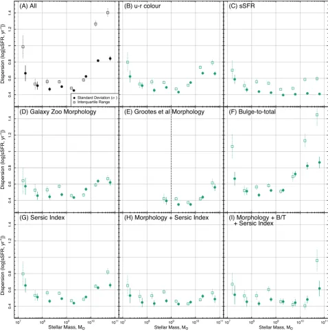
4 A M A S S D E P E N D E N T σS S F R?

Using each of the sample selection methods described above, we

exploreσsSFRas a function of stellar mass. Here, we defineσsSFR

as the standard deviation of log10[sSFR] for the selected population

at a given stellar mass. Note that following this we also calculate

the dispersion based on the interquartile range of log10[sSFR], to

remove any dependencies on assumption of a Gaussian-like distri-bution.

We take all of our selected galaxies (black points in Fig.2A, and

green points in Fig.2B-I) and split our samples into log10[M∗/M]

=0.5 bins of stellar mass. Fig.3displays an example of the

distri-bution of galaxies away from the median in each bin with Poisson

errors, for bothMAGPHYSand HαSFRs. For this figure, we only

show sources identified as disc like from our combined Galaxy Zoo morphology and S´ersic index selection (i.e. the population in Panel

H of Fig.2). This shows the spread of sSFRs away from the locus

of the SFS at a given stellar mass.

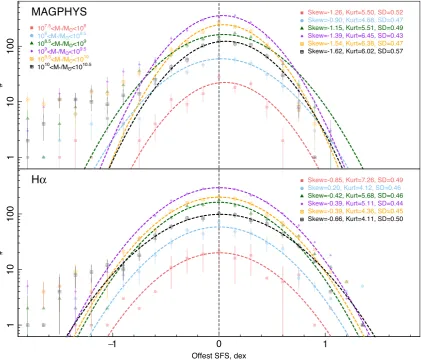
For illustrative purposes only, in Fig.3we fit a lognormal in each

mass bin (dashed lines) to highlight any deviation in the popula-tion from a symmetric lognormal distribupopula-tion. Unsurprisingly, at all masses we see an asymmetric tail extending to low sSFRs in-dicative of a green-valley/passive population (also see Oemler et al.

2017). We also potentially see an additional star-burst population

1

10

100

#

Skew=-1.26, Kurt=5.50, SD=0.52

Skew=-0.90, Kurt=4.68, SD=0.47

Skew=-1.15, Kurt=5.51, SD=0.49

Skew=-1.39, Kurt=6.45, SD=0.43

Skew=-1.54, Kurt=6.38, SD=0.47

Skew=-1.62, Kurt=6.02, SD=0.57

107.5<M*/Mʘ<10 8

108<M*/Mʘ<10

8.5

108.5_<M */Mʘ<109

109<M*/Mʘ<10 9.5

109.5<M*/Mʘ<10 10

1010_<M

*/Mʘ<1010.5

MAGPHYS

−1 0 1

1

10

100

Offest SFS, dex

#

Skew=-0.85, Kurt=7.26, SD=0.49

Skew=0.20, Kurt=4.12, SD=0.46

Skew=-0.42, Kurt=5.68, SD=0.46

Skew=-0.39, Kurt=5.11, SD=0.44

Skew=-0.39, Kurt=4.36, SD=0.45

Skew=-0.66, Kurt=4.11, SD=0.50

H

α

Figure 3. The distribution of points away from the SFS isolated using the combined morphology+S´ersic index selection from Section 3.4. We display the distribution in stellar mass bins for bothMAGPHYSand Hαderived SFRs. Points are fit with a lognormal distribution (dashed lines) to highlight any deviation from this symmetric shape. In both SFRs and at all masses, the distributions display a negative skew value, highlighting that the distributions have asymmetric tails extending to low stellar masses. For both SFRs in all but the lowest stellar mass bin, the skew value becomes more negative to higher stellar masses suggesting that the distribution becomes more asymmetric as a function of mass.

in the Hαdistribution at high SFRs (particularly seen in the

posi-tive kurtosis of the 8<log10[M∗/M]<9 bin). This is interesting

as it may provide evidence of short duration star-burst activity; as

Hαprobes star formation integrated over shorter time-scales than

MAGPHYS(see Davies et al.2015b). This will be explored further in later papers of this series.

To determine how these distributions vary as a function of stellar mass, we calculate the skewness, kurtosis, and standard deviation

of log10[sSFRs] in each mass bin; given in the legend of Fig. 3.

Interestingly, with the exception of the 8.0<log10[M∗/M]<8.5

bin in Hα, all distributions show a negative skew (from the green

valley/passive population) but with skewness increasing for higher

stellar masses for bins at log10[M∗/M]>8.0. Tentatively, this may

indicate that any physical processes that drive the shape of this dis-tribution are more likely to produce more symmetrical scatter at the low-mass end (potentially stochastic star formation bursts leading to stellar feedback), and asymmetrical scatter at the high-mass end (po-tentially AGN feedback). However, care must be taken as we may simply be missing a significant fraction of the quenched population at low stellar masses, and artificially removing the asymmetric tail due to selection affects imposed by GAMA. In order to go further,

we require much deeper spectroscopic surveys of the local Uni-verse, such as the Wide Area VISTA Extragalactic Survey (WAVES

Driver et al.2016b), which will allow a detailed exploration of the

distribution of star formation in very low-mass galaxies.

Taking this further, we then use the standard deviation

measure-ments described above to derive the σsSFR–M∗ and measure the

interquartile range in the same stellar mass bins; for all selections described in Section 3.

Fig.4displaysσsSFR (filled circles) and the interquartile range

(open squares) in log10[M∗/M] = 0.5 bins of stellar mass

fol-lowing the same panel layout as Fig.2. Here, we only show

fig-ures for MAGPHYSSFRs, but similar figures for other SFR

indi-cators are given in the Appendix. Statistical errors on σsSFR are

calculated as

ErrσsSFR_i ∼

2σ4

sSFRi(Ni−1)

−1

2σsSFRi

, (4)

whereiis the index of the stellar mass bin andNis the number of

galaxies in that bin (Rao1973). We then combine this in

quadra-ture with the error calculated from 100 bootstrap resamples of the

0.4

0

.6

0.8

11

.2

1

.4

Dispersion (log[sSFR, yr

−

1])

Standard Deviation (σ) Interquartile Range

(A) All (B) u-r colour (C) sSFR

0.4

0

.6

0.8

11

.2

1

.4

Dispersion (log[sSFR, yr

−

1])

(D) Galaxy Zoo Morphology (E) Grootes et al Morphology (F) Bulge-to-total

107 108 109 1010 1011

0.4

0

.6

0.8

11

.2

1

.4

StellarMass,Mʘ

Dispersion (log[sSFR, yr

−

1])

(G) Sersic Index

107 108 109 1010 1011

StellarMass,Mʘ (H) Morphology + Sersic Index

107 108 109 1010 1011

StellarMass,Mʘ (I) Morphology + B/T

+ Sersic Index

Figure 4. The resultant dispersion along the sSFR–M_∗relation measured using both the standard deviation (σsSFR–M∗, filled circles) and interquartile range (open squares). Each panel shows a different method for isolating the SFS described in Section 3. This Figure follows the same layout as Fig.2, but only using SFS-selected population (green points when both green and red are present in Fig.2). While the normalization and shape changes, the majority distributions show a ‘U’-shaped dispersion with minimum at∼109_{.25 M}

and increased scatter at low and high masses for bothσsSFRand interquartile range.

population within the errors of both stellar mass and SFR. For errors on the interquartile range, we only apply the bootstrap resampling errors. This bootstrap resampling is intended to take into account the varying measurement error in each of our SFR indicators as a function of stellar mass.

First, we find that the majority of the panels show close to

‘U’-shaped distribution with minima atσsSFR∼0.35–0.5 dex and

log10[M∗/M] = 8.5–9.5 (in the following section, we fit these

distributions with a second-order polynomial to find the minimum

points). We observe a steep increase in bothσsSFRand interquartile

range to higher stellar masses than this minima. The increase to

lower stellar masses is much shallower but tentatively observable in both measures of dispersion. These results are roughly

consis-tent with observations of Guo et al. (2015) and Willett et al. (2015)

modulo slight differences in normalization (∼0.1 dex) and have

comparable scatter to the recent results of Boogaard et al. (2018).

We also find a consistency between the dispersion measured using

bothσsSFRand the interquartile range at most stellar masses, this

indicates that the assumption of a lognormal distribution of sSFRs at a given stellar mass is appropriate. The places where this does not hold true are when stellar masses are either very low or very

high (this is also displayed in the larger kurtosis values in Fig.3).

In these regimes, the interquartile range may be a more accurate representation of the dispersion as it does not assume a lognormal distribution.

We find that while sample selection does affect the normalization of the dispersion at specific stellar masses, we do see consistency between sample selections in terms of the minimum point in both stellar mass and dispersion, and in the overall shape; with all samples displaying a dispersion that rises to low and high stellar masses.

We also find that when selecting on sSFR (panel C) we observe

a more linear distribution with decreasingσsSFRto higher stellar

masses. This is as expected as a hard cut in sSFR simply removes the high-dispersion population at high stellar masses (see panel C of

Fig.2). In combination, the panels in Fig.4suggest that irrespective

of the method for selecting a star-forming/disc-like galaxy popu-lation based on colour and morphology, in GAMA we observe a

‘U’-shapedσsSFR–M∗relation, which is largely consistent with the

previous observations of Guo et al. (2015) and Willett et al. (2015).

4.0.1 Mixture modelling method

In addition to the physically motivated sample selections described

previously, it is also possible to determine theσsSFR–M∗ relation

based on mixture modelling of the star-forming and passive

population (see Taylor et al.2015, for a similar approach). Here,

we use the [R] MIXTOOLS:NORMALMIXEM function to perform

a maximum log-likelihood mixture fit to the two population in

log10[M∗/M] =0.5 bins of stellar mass at log10[M∗/M]>8.5

(below this we assume a single high-sSFR population). The top

panel of Fig.5shows the sSFR–M_∗ plane forMAGPHYS-derived

SFRs. The green and red lines display the mean (solid lines) and

1σ width (dashed lines) of the mixture models for the high-sSFR

and low-sSFR population, respectively.

The bottom panel of Fig. 5then showsσsSFR–M∗ relation for

the high-sSFR population, where errors are calculated using

equa-tion (4) but whereNis the number of galaxies in a particular stellar

mass bin multiplied by the mixing proportion in the high-sSFR pop-ulation. Once again we find a ‘U’-shaped distribution with minima

at log10[M∗/M]∼9.25 andσsSFRincreasing to low and high stellar

masses. We do find that the normalization of theσsSFR–M∗relation

for our mixtures is slightly lower than for our previous selections

(minima atσsSFR∼0.3 dex), likely due to the fact that large

dis-persion points are included in the low-sSFR mixture irrespective of their physical properties.

However, it is interesting to highlight that when using non-physically motivated separation between the star-forming and

pas-sive population we still observe a ‘U’-shapedσsSFR–M∗. This result

is therefore once again, unlikely to be driven by choice of sample selection.

4.1 Variation with SFR indicator

We also consider if the results described above hold true for differ-ent SFR indicators; as differdiffer-ent observables can provide differdiffer-ent

measures of star formation with varying degrees of scatter (e.g.see

Davies et al.2016). In addition, other explorations into the

disper-sion along the SFS have used a number of different SFR indicators. As such, we wish to produce a comparison point to these studies from GAMA in the local Universe.

Hence, we reproduce our analysis for all other SFR indicators

dis-cussed in Section 2.1.1. Figures identical to Figs2and4are given in

the appendix for UV+TIR, Hα, W3, andu-band SFRs. In the

ma-jority of cases, these figures display a largely ‘U’-shapedσsSFR–M∗

10

−

13

10

−

12

10

−

11

10

−

10

10

−

9

10

−

8

sSFR, yr

−

1

High sSFR population +/-sigma Low sSFR population +/-sigma

107 108 109 1010 1011

0.2

0

.4

0.6

0.8

StellarMass,Mʘ

σsSFR

, dex

Figure 5. Mixture modelling of the star-forming and passive population assuming lognormal distributions in sSFR. The top panel displays the SFR– M∗plane forMAGPHYS-derived SFRs. The green and red lines display the mean (solid lines) and 1σ width (dashed lines) of the mixture models as a function of stellar mass. The bottom panel shows theσsSFR–M∗relation for

the high-sSFR population.

relation with minimum atσsSFR∼0.35–0.5 dex and log10[M∗/M]

=9–10. They all display a steep increase of dispersion to high

stel-lar masses, and a more tentative, shallow increase to lower stelstel-lar masses.

The u-band SFRs (Fig.A4) do have a much smaller dispersion

across all stellar masses (minimum at σsSFR ∼ 0.2–0.3 dex) but

retain a ‘U’-shape. The changes in normalization ofσsSFRbetween

SFR indicator are likely due to the robustness of each indicator in measuring SFRs and how correlated they are with stellar mass; with high scatter indicative of larger measurement error and/or unknown assumptions in converting from an observable to a true SFR (e.g.

see Davies et al.2016).

In Fig. A5, we produce a comparison of all SFR indicators

by scaling the distributions using the minimum dispersion in each indicator. This removes some of the dependence on absolute

(A)

(D)

(E)

(B)

(C)

Figure 6. The high-mass and low-mass slope of theσsSFR–M∗relation for different SFR indicators (described in Section 2.1.1) and using each method for isolating the SFS (described in Section 3). We separate theσsSFR–M∗distributions in Fig.A5and take the high-mass end as log10[M∗/M]>9.25 and low-mass end as log10[M∗/M]<9.25. We then linearly fit the slope at high (squares) and low masses (circles) – see bottom right-hand panel. Each other panel displays a different SFR indicator, and each pair of points/line displays a different method for isolating the SFS. In this figure, when the pair of points spans the dashed zero line, the distributionσsSFR–M∗is parabolic with a minimum vertex, when they both sit below the dashed zero lineσsSFRdecreases

with mass, and when they both sit above the dashed zero lineσsSFRincreases with mass. The size of the distance between the two points is indicative of how

curved the distribution is about log10[M∗/M]=9.25. Note that for the Grootes et al. morphological proxy, we only have the high-mass slope. We find that in almost all cases theσsSFR–M∗relation is parabolic (the pairs of points span the dashed zero line). We also note that if we use either log10[M∗/M]=8.75 or log10[M∗/M]=9.75 as our minimum points it does not significantly alter these results.

normalization between SFR indicators and allows a more direct comparison of their shape. In the majority of cases, each indicator shows a ‘U-shape’ with largely consistent increases in dispersion to low and high stellar masses, irrespective of SFR used. The most

notable exception to this is the UV+TIR indicator. This is largely

due to the tfact hat the minimum point inσsSFR occurs at higher

stellar masses for this indicator (close to log10[M∗/M] =10).

In order to easily compare the shape of theσsSFR–M∗relation

for all SFR indicators and sample selections, we define a simple

metric based on the slope ofσsSFR–M∗in the low- and high-stellar

mass regime; divided at log10[M∗/M] = 9.25. To choose this

reference point, we fit a second-order polynomial to theσsSFR–M∗

relation for all samples and SFR indicators and find the median

minimum point to be at log10[M∗/M] =9.261, hence our closest

stellar mass bin is log10[M∗/M] = 9.25. We then perform a

least-squares linear fit to the low-mass and high-massσsSFR–M∗,

respectively. This process is described visually in the bottom

right-hand panel of Fig.6. While the point at log10[M∗/M] =9.25 does

not represent the minimum in all distributions (see above), we wish

to use a consistent point across allσsSFR–M∗relations to highlight

any variation with sample selection and/or SFR indicator. However,

we do repeat this analysis for slopes about both log10[M∗/M]

=8.75 and log10[M∗/M]=9.75 and find consistent results. While

this is potentially a crude metric for the shape of the distributions, it allows an easy comparison of multiple different samples in the same figure.

Fig.6displays these low- and high-mass slopes for each sample

selection (colours) and for each SFR indicator (panels). In this

figure, points that span they=0 line have a ‘U’-shaped distribution.

In addition, the separation between the points (length of the coloured lines) describes how curved the distribution is, with points close together indicating a linear relation, and far apart a highly curved

distribution. For samples that cross they=0 line, the position where

the coloured line crosses they= 0 line describes the asymmetry

of the distribution about log10[M∗/M] =9.25. For example, a

purely symmetric ‘U’-shape would have widely vertically spaced

points with the dashed y= 0 crossing at the mid-point of their

connecting line.

From this figure, we see that the majority of our samples have

widely separated points that span the y = 0 line. This metric

displays, at a glance, that irrespective of sample selection or SFR

indicator theσsSFR–M∗relation is U’-shaped with minimum close

to log10[M∗/M]=9.25 and increasing dispersion to low and high

stellar masses. The exception to this is the selection using sSFR that

107 108 109 1010 1011

0

0

.2

0.4

0

.6

0.8

1

StellarMass,Mʘ

σsSFR

, dex

(A) All

EAGLE (All) Shark-Medi (All) Shark-Micro (All) MAGPHYS

UV+TIR Hα

W3 u-band

107 108 109 1010 1011

StellarMass,Mʘ

(C) sSFR

EAGLE (sSFR cut) Shark-Medi (sSFR cut) Shark-Micro (sSFR cut)

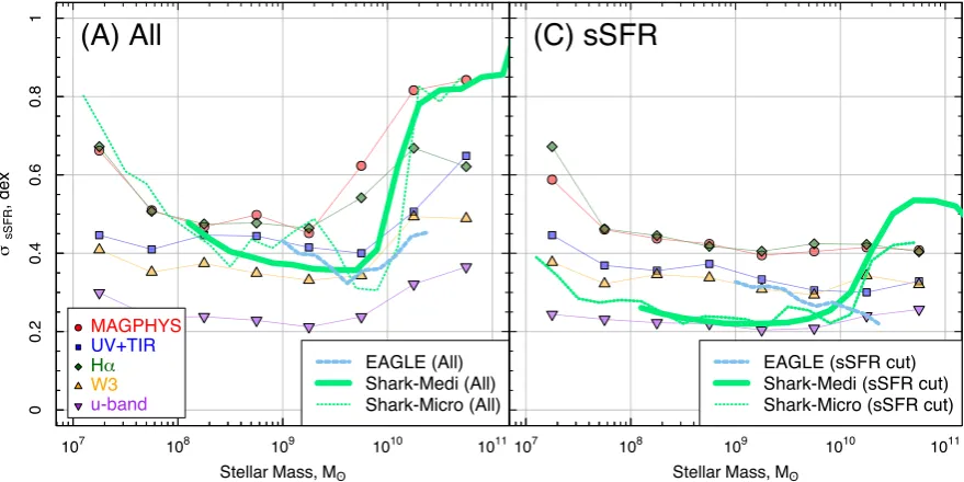
Figure 7. σsSFR–M∗relation from the Shark SAM (solid green) compared to our observations for different SFR indicators (coloured points) and the EAGLE simulation results (dashed blue lines). The left-hand panel displays the relation for all galaxies, while the right-hand panel shows only galaxies with log10[sSFR,

yr−1_{]>−11. Both simulations are only shown above their mass resolution limits. Shark displays a remarkably similar distribution to our data in the left-hand}

panel, and both Shark and EAGLE show a similar relation but offset slightly in normalization in the right-hand panel at log10[M∗/M]<10. At the highest

stellar masses, we see an upturn for Shark, which is not found in EAGLE or the observations; due to that fact that in Shark, star formation in very massive galaxies declines slowly and galaxies stay above the sSFR cut.

has a linearly decreasing dispersion with stellar mass in the majority

of cases (both points sit below the y =0 line). Once again this is

expected as the cut in sSFR removes the large dispersion population at high stellar masses.

4.2 Comparison to the state-of-the-art semi-analytic model and hydrodynamical simulations

In addition to the Katsianis et al. (in preparation) results from

EA-GLE discussed previously, we also compare our observedσsSFR–

M_∗relation to the state-of-the-art SAM Shark (Lagos et al.2018).

Briefly, Shark is a highly flexible and modular open-source SAM, which includes several different models for gas cooling, AGN, stel-lar and photoionization feedback, and star formation. Here, we use

the Shark parameters described in Lagos et al. (2018) run over the

SURFS (Elahi et al.2018) simulations with Planck15 cosmology

and take the Shark+SURFS galaxies in the z =0 shapshot. We

use both the medi-SURFS (medium box size and medium mass resolution) and mircro-SURFS (small box size and high-mass res-olution) simulation runs (we do not go into further details of the

simulations here, for more details see Elahi et al.2018and Lagos

et al.2018). Using the Shark-simulated galaxies, initially we take

all isolated central galaxies (as in GAMA) and bin in stellar mass

bins of log10[M∗/M] =0.2 dex. We then calculate the standard

deviation of sSFRs in each bin (consistent with our observational data). For details of the EAGLE results and in-depth discussion of

the EAGLEσsSFR–M∗relation, see Katsianis et al. (in preparation).

The left-hand panel of Fig.7displays theσsSFR–M∗relation using

all SFR indicators used in this work for all isolated galaxies overlaid with the relations measured from both Shark and EAGLE (Note that for EAGLE we also only include all isolated central galaxies at z

∼ 0). We find that theσsSFR–M∗ relation from both simulations

are consistent with the GAMA results; showing a ‘U’ shape with

minimum at log10[M∗/M]=9–10 and a steep rise at higher stellar

masses (albeit only over a small stellar mass range for EAGLE). We also highlight the gradual rise to lower stellar masses in the Shark results, which is observed in some of our SFR indicators. This falls below the mass resolution limit for EAGLE.

We also replicate the sample with a log10[sSFR, yr−1]>−11 cut

(right-hand panel of Fig.7), where both EAGLE and Shark follow

a similar relation to the observational data at low to intermediate stellar masses, which sits within the spread of the different SFR indicators explored here. At the highest stellar masses, we still see

an upturn inσsSFRfor Shark, which is not found in EAGLE or the

observations. This is due to the fact that in Shark, star formation in very massive galaxies declines slowly and galaxies stay above the sSFR cut. In EAGLE, massive galaxies tend to quench rapidly, dropping below the sSFR cut. We also note that the EAGLE mass

resolution is limited at log10[M∗/M]∼9 and the resolution limit

for Shark is log10[M∗/M]∼8 for medi-SURFS and log10[M∗/M]

∼7 for micro-SURFS.

In summary, the Shark model reproduces the observedσsSFR–M∗

relation across all stellar masses incredibly well given that it was not specifically tuned to reproduce the dispersion in this plane, while EAGLE reproduces the relation well above its resolution limit. We note here again that within EAGLE, Katsianis et al. (in preparation) attribute the high dispersion at low and high stellar masses to stellar and AGN feedback, respectively. It is worth highlighting that both EAGLE and Shark use a physical model for AGN and stellar feed-back (i.e. not a simple mass scaling that may artificially produce

these results). In addition, Lagos et al. (2018) showed that the scatter

of the SFS is very sensitive to the adopted star formation law; that is both the way that the interstellar medium is partitioned between ion-ized, atomic, and molecular gas, and the way molecular gas is con-verted into stars. Various theoretical and empirical models for star

formation were used leading to>0.2 dex differences inσsSFR. These

results suggest that the interplay between gas/stars within the galaxy

can also play a significant role in shaping theσsSFR–M∗relation.

−

0.3

−

0.2

−

0.1

0

0.1

0

.2

0.3

SFS-selection

Slope

σ

sSFR

All

Increasing with mass

u-shaped

Decreasing with mass

(A) MAGPHYS

u-r

SFR

Disk (Zoo)

Disk (Grootes) B/T

Sersic

Disk+Sersic

Disk+BT+Sersic

−

0.3

−

0.2

−

0.1

0

0.1

0

.2

0.3

SFS-selection

Slope

σ

sSFR

All

M*<10 9.25

Mʘ slope M*>10

9.25 Mʘ slope

(C) H

α

u-r

SFR

Disk (Zoo)

Disk (Grootes)

B/T

Sersic

Disk+Sersic

Disk+BT+Sersic

108 109 1010 1011

00

.1

0

.2

0.3

0

.4

StellarMass,Mʘ

Δ σ

sSFR

(group-isolated)

(A) MAGPHYS

u-r

sSFR

Disk (Zoo) Disk (Grootes)

B/T

Sersic

Disk+Sersic

Disk+B/T+Sersic

108 109 1010 1011

00

.1

0

.2

0.3

0

.4

StellarMass,Mʘ

Δ

σsSFR

(group-isolated)

(C) H

α

Figure 8. Top: The same diagnostic displayed in Fig.6but for justMAGPHYSand Hα-derived SFRs in group satellite galaxies. The differences between these panels and Fig.6highlight additional sources of scatter in theσsSFR–M∗relation in groups (see text for details). Bottom: The relative difference betweenσsSFR

for group satellites andσsSFRfor isolated galaxies in three stellar mass bins. We find increased dispersion in group satellites at all stellar masses (σsSFR>

0), which is more extreme at low and intermediate masses.

4.3 The impact of group environment

Finally, we consider the impact of group-scale environments on

the metric used to parametrize the shape of theσsSFR–M∗relation

in Section 4.1. Differences between these metrics for isolated and group environments can potentially elucidate additional physical

sources of dispersion in the sSFR–M_∗ relation caused by group

astrophysical processes. To reduce confusion in the number of

sam-ples displayed, in this section we will only focus onMAGPHYSand

Hα-derived SFRs.

To explore the effect of group environment, we select all galaxies

within our volume-limited samples that are in an N> 2 group

from the GAMA group catalogue of Robotham et al. (2011). We

then exclude all sources that are closest to the iterative centre of the group as a central. The remaining sources form our ‘group satellites’ sample, for which we repeat all of the analysis in the previous sections.

The top row of Fig.8displays the same metric as in Fig.6but for

the group satellites. There are two notable differences: (i) the pairs of points for each sample selection are closer together indicating that the distribution is less curved, and (ii) the points are more negative both at the high- (squares) and low- (circles) mass end indicating that in most cases the distributions are no longer ‘U’ shaped but

have a decreasingσsSFRwith increasing stellar mass.

However, the top row of Fig.8does not inform as to whether

the observed changes are caused by the dispersion increasing or de-creasing in group environments, only that the relative shape of the

σsSFR–M∗relation changes. To explore this further, the bottom row

of Fig.8displays the normalization difference ofσsSFRbetween the

isolated and group satellite samples at three stellar mass bins (i.e. for each independent sample selection and SFR indicator we measure

the offset between log10[σsSFR] in isolated and group environments

at log10[M∗/M]=8.25, 9.25, and 10.25). We find thatσsSFRis

larger in group satellites than in isolated galaxies for all samples

107 ₁₀8 ₁₀9 ₁₀10

Stellar Mass, M

0.2

0.4

0.6

0.8

1.0

σsSFR

, dex

Isolated

Groups - MAGPHYS

Groups - H

Incr

eased

Sca

tter

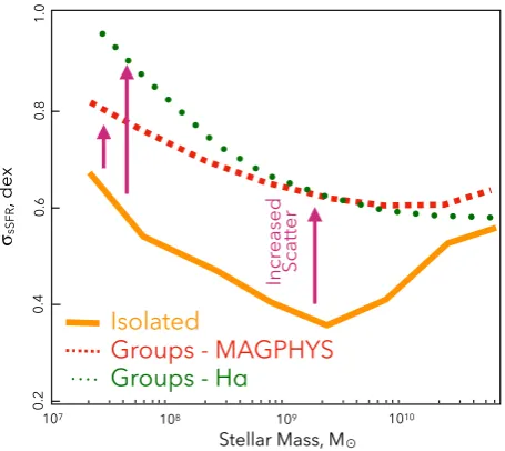
Figure 9. Cartoon representation of the differences in observedσsSFR–M∗

relation between isolated and group environments. The parabolic distribution observed in isolated galaxies is removed by additional large dispersion at low and intermediate stellar masses.

and at all stellar masses (i.e. all points are above zero), but that the increase in dispersion is much larger at low and intermediate stellar masses than at high stellar masses. This indicates that group

envi-ronments preferentially increaseσsSFRfor low-mass galaxies, likely

due to increased satellite quenching low-mass galaxies leading to increased dispersion (this is explored in detail in Davies et al., in

preparation). To highlight this, Fig.9shows a cartoon

representa-tion of how theσsSFR–M∗ relation changes between isolated and

group satellite galaxies.

To explore the population that is driving the observed differences between isolated galaxies and group satellites further, we return to

the full sSFR–M_∗plane and compare the distribution of sources in

each environment. Fig.10displays the HαandMAGPHYSsSFR–M_∗

plane for isolated galaxies (top rows) and group satellites (bottom row) selected as disc-like systems using the combined Galaxy Zoo morphology and S´ersic index selection. The dashed vertical lines display the points at which we measure the normalization difference

inσsSFRfor Fig.8.

First, we find that there is uniformly larger dispersion along the SFS population at all stellar masses in groups; potentially due to more stochastic star formation processes occurring in groups via interactions. We also find an additional population of quenched

group satellite galaxies at log10[M∗/M]∼9–10. To highlight this,

in Fig.10we colour all galaxies with sSFRHα <10−11.2 in red.

This population increasesσsSFRat the point whereσsSFR–M∗is a

minimum in isolated galaxies, removing the ‘U’-shape shape. This population is likely produced by group-quenching processes (such as strangulation/starvation/stripping). We leave detailed discussion of potential physical mechanisms that may produce these population to the following papers in this series.

However, interestingly we note that this population sits on a

tight sequence when using Hα-derived SFRs, but is much more

dispersed to higher sSFR when usingMAGPHYS-derived SFRs. This

potentially indicates that group satellites that appear passive in Hα

-derived SFRs are still transitioning across the green valley when

usingMAGPHYS-derived SFRs. There are two important differences

between SFRs measured using these indicators: (i) GAMA Hα

SFRs are derived from fibre-fed spectroscopy and therefore only

probe the central regions of galaxies, while MAGPHYS SFRs are

integrated over the whole galaxy, and (ii) HαSFRs probe a much

shorter integrated physical time-scale than MAGPHYS SFRs (i.e.

<20 Myr as compared to<100 Myr, e.g. Davies et al.2015a). The

differences in the red points in different columns of Fig.10could

be attributed to sources that have quenched on short time-scales, and thus still have residual star formation when measured using

MAGPHYS, or sources that are undergoing inside-out quenching and thus become completely passive over the central regions observed by our fibre-fed spectroscopy prior to the whole galaxy becoming passive. We leave detailed discussion of these mechanisms to the following papers, where we aim to produce a more complete picture

of the sSFR–M_∗plane based on multiple observations.

5 C O N C L U S I O N S

In the first paper of this series, we have parametrized the dispersion along the SFS for different sample selections and SFR indicators within GAMA. We find that

(i) Irrespective of selection method of star-forming disc-like

sys-tems, the σsSFR–M∗ relation is parabolic with high dispersion at

the low and high stellar mass end and minimum point of σsSFR

∼0.35–0.5 dex at log10[M∗/M]∼8.75–9.75. This holds true for

different SFR indicators and when using mixture modelling, albeit

with differences in normalization ofσsSFR.

(ii) Our results are largely consistent with a number of previous studies and simulation results from EAGLE, Illustris, and Shark. The EAGLE study suggests that this parabolic dispersion is pro-duced via stellar and AGN feedback at the low- and high-mass end, respectively, while Shark suggests that the interplay between gas/stars within the galaxy can also play a significant role in shap-ing the dispersion. This will be explored further observationally in subsequent papers in this series.

(iii) In combination, these results suggest that the ‘U’ shape of

σsSFR–M∗relation is physical and not an artefact of sample selection

or method.

(iv) For group satellite galaxies, we find an increased dispersion at all stellar masses potentially due to more stochastic star formation processes occurring in groups. We also find an additional population

of quenched sources at log10[M∗/M] ∼ 9–10, which increases

σsSFRand removes the parabolic shape.

(v) We tentatively suggest that this population is produced by group-quenching processes and highlight that differences between

Hα- andMAGPHYS-derived SFRs for this population may be

in-dicative of short time-scale quenching. However, we leave detailed discussion to the following papers.

We have parametrized the σsSFR–M∗ relation in the local

Universe and highlighted that it is a useful tool in exploring the recent SFH of galaxies both in terms of the variation of dispersion as a function of stellar mass and in the differences between isolated galaxies and group satellites. In the following papers in this series,

we will explore the morphological evolution across the sSFR–M_∗

plane and the physical processes that drive the formation of this fundamental relation.

AC K N OW L E D G E M E N T S

GAMA is a joint European–Australian project based around a spec-troscopic campaign using the Anglo- Australian Telescope. The