Multivariate analysis of 3D ToF SIMS images: method validation and application to cultured neuronal networks

(1)

COMMUNICATION

Cite this:DOI: 10.1039/c5an01743b

Received 26th August 2015, Accepted 20th November 2015

DOI: 10.1039/c5an01743b

www.rsc.org/analyst

Multivariate analysis of 3D ToF-SIMS images:

method validation and application to cultured

neuronal networks

†

S. Van Nu

ﬀ

el,

a,b

C. Parmenter,

c

D. J. Scurr,

a

N. A. Russell

b

and M. Zelzer*

a,d

Advanced data analysis tools are crucial for the application of

ToF-SIMS analysis to biological samples. Here, we demonstrate that by using a training set approach principal components analysis (PCA) can be performed on large 3D ToF-SIMS images of neuronal

cell cultures. The method readily provides access to sample com-ponent information and signi_ﬁcantly improves the images_’ signal-to-noise ratio (SNR).

Time-of-Flight Secondary Ion Mass Spectrometry (ToF-SIMS) is capable of generating 3D chemical-composition images by com-bining label-free, 2D molecular imaging with depth profilingvia ion beam sputtering. The technique has proven its ability to characterise surfaces and coatings of inorganic and organic materials,1 _{and is increasingly used for pharmaceutical}

appli-cations.2_{In particular, the research on 3D ToF-SIMS imaging of}

single cells has progressed to the point where the intracellular uptake and location of non-native compounds such as bromo-deoxyuridine3_{and amiodarone}4_{can be imaged.}

Despite the increasing capabilities of ToF-SIMS instru-ments, typical ToF-SIMS measurements have a number of fundamental limitations that make data acquisition and interpretation challenging.5_{Chief among these is the intrinsic}

trade-oﬀ between high mass resolution and high spatial resolution. Analysis in the static regime limits the signal-to-noise ratio as no more than 1% of the surface can be bom-barded with primary ions in order to avoid hitting sites damaged by the analysis beam, which means only a very small fraction of the sample is used for analysis. The low duty cycle of the pulsed ion beam leads to long depth profiling

experi-ments, which frequently causes samples to be analysed well below the static limit as well, in order to save time. Addition-ally, the ion images of high-mass molecular species often have a poor signal-to-noise ratio due to the low ion count per pixel.6

There are also complications involving the secondary ion yield, when the sample material has a curvature or a surface topogra-phy in excess of several tens of µm.7_{The analysis of biological}

samples is particularly aﬀected by these limitations. Because of their inherent complexity and the close chemical similarities of most of the compounds of interest ( proteins, lipids and carbo-hydrates), biological samples require a high mass resolution. At the same time, cellular features are relatively small (sub-micrometer range) compared to current ToF-SIMS lateral resolu-tion limits (commonly in the µm range although sub-µm is possible). The compounds of interest also usually generate high-mass species, which have a poor signal-to-noise ratio. Finally, biological samples can show curvature and surface topo-graphy to the extent, where they aﬀect the secondary ion yield.

With these limitations in mind, powerful data analysis is of the essence, which is why the SIMS community has embraced multivariate analysis (MVA) methods such as PCA.8_{While PCA}

already proved useful for 2D ToF-SIMS image analysis, 3D ToF-SIMS data sets are typically very large and unsuitable for MVA using the processing power of standard desk top compu-ters.5_{As a result, up until now the only published application}

of PCA on a 3D ToF-SIMS dataset was reported by Fletcher et al.9_{on a relatively small 3D ToF-SIMS image with a size of}

256 × 256 × 10 pixels. Very recently, Cumpsonet al.10

develo-ped faster algorithms that allowed PCA to be performed on large 2D data sets. Here, we demonstrate that it is possible to expand the application of PCA to large (256 × 256 × 160) 3D images under 30 minutes without requiring any computing resources beyond a desk top computer. We used a small train-ing subset compristrain-ing 6.1% of the total amount of pixels, which were randomly selected from the full 3D image, to deter-mine the PCA loadings (i.e.linear combinations of the original mass peaks accounting for amounts of variance). These load-ings were then applied to the full data set. We have validated our method using an established data set with known

compo-†Electronic supplementary information (ESI) available. See DOI: 10.1039/ c5an01743b

a_{Laboratory of Biophysics and Surface Analysis, School of Pharmacy, Boots Science}

Building, University of Nottingham, University Park, Nottingham NG72RD, UK

b_{Neurophotonics Lab, Faculty of Engineering, University of Nottingham, University}

Park, Nottingham NG72RD, UK

c

Nottingham Nanotechnology and Nanoscience Centre, University of Nottingham, University Park, NG72RD, UK

d

National Physical Laboratory, Teddington, Middlesex, TW110LW, UK. E-mail: [email protected]

Open Access Article. Published on 20 November 2015. Downloaded on 10/12/2015 15:57:55.

This article is licensed under a

Creative Commons Attribution 3.0 Unported Licence.

(2)

sition and distribution that was previously published11before applying it to a 3D ToF-SIMS data set of a primary, embryonic rat cortical cell culture.

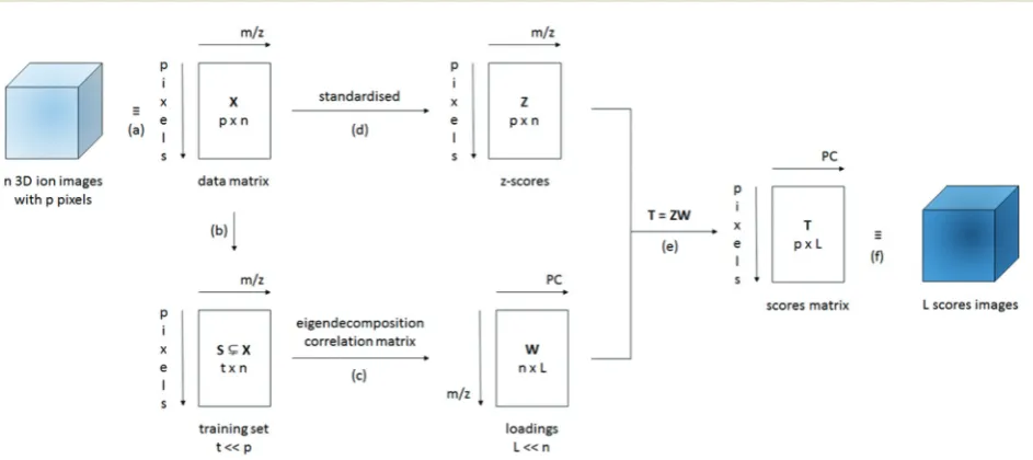
PCA is a technique that allows the variables in a data set to be reduced to a few, interpretable linear combinations of those variables. In the case of ToF-SIMS images, the mass peaks are regarded as variables and each pixel as an individual obser-vation or sample; the aim is to reduce the hundreds of ion images to a few, interpretable images of the principal com-ponent scores. A simplified schematic of our data processing method for large 3D ToF-SIMS images is shown in Fig. 1. After a peak search to identify the relevant mass peaks, the respect-ive secondary ion images are imported into Matlab (Release 2013a, The MathWorks, Inc., Natick, Massachusetts, United States) and reshaped into (scan resolved) matrices, where the rows represent pixels (or samples) and the columns represent mass peaks (or variables). Normalisation with the total ion count per pixel or the sum of the selected peaks is an option at this point in case one would like to minimise variations in the secondary ion signal due to differences in topography, sample charging or instrumental conditions such as variations in primary ion current or detector efficiency.12,14All data sets presented here are normalised prior to analysis. Because the eigendecomposition involved is computationally intensive, a smaller training subset of randomly selected pixels is created to calculate the principal component coefficients (i.e.the load-ings). Depending on whether the covariance or the correlation matrix of the training set is decomposed, the data is either mean-centered or standardised (auto-scaled) respectively.

Because the correlation coefficients are obtained by dividing the covariance of the variables by the product of their standard deviations, the correlation matrix is equal to the covariance matrix of the standardized data. When mean-centering, PCA will give more weight to variables that have higher variances, which tend to be the variables with higher means. If the vari-ables are standardised, all varivari-ables will be weighted equally regardless of how abundant they are. It is important to note that standardisation has a tendency to amplify noise peaks relative to peaks which show image contrast8and is therefore not generally recommended over scaling methods that are con-sistent with the structure of the noise. Root mean scaling, derived from the assumption that the image noise is Poisson in nature, often yields better results. However, this is not the case when the Poisson assumption is badly violated, which occurs when the data is normalized.8 While the (corrected) sample standard deviation is a biased estimator for the popu-lation standard deviation, its bias drops offas 1/Nas sample size increases. Given the size of the training sets used and the fact that the sample standard deviation makes no assumptions regarding the distribution, scaling using the sample standard deviation was chosen. The training set data presented here has always been standardised. The full data matrix then needs to be standardised and multiplied with the loadings in order to calculate the scores for every pixel in the image. This can be done efficiently one scan at a time (block processing).

To validate the method, we are using a previously pub-lished11model 3D ToF-SIMS data set of a spin-cast multilayer sample comprising ten well-defined, alternating layers of

Fig. 1 Simpli_ﬁed schematic of the data processing method used. (a) The n di_ﬀerent 3D (normalised) ion images for every_m/_zcan be presented as a data matrixXwith n columns (one for every_m/_z) and p rows (one for every_xyzpixel). (b) In order to calculate the loadings matrixWof the L (_≪n) principal components, a smaller training data setSwith t (_≪p) randomly selected pixels is created; the training setS(t × n) is a subset of the data matrixX( p × n). (c) Eigendecomposition of the correlation matrix ofS, provides the loadings matrixWwith L columns (one for every PC) and n rows (one for every_m/_z). (d) Because the training setSwas standardised for the calculation of the loadingsW, the data matrixXhas to be standardised as well using the mean and standard deviation for each column n of the training setSgenerating the z-scores matrixZ( p × n). (e) The scores matrixT

with L columns and p rows is calculated as the matrix product ofZ( p × n) andW(n× L). (f ) The scores matrixTcan now be presented in the form of L (_≪n) interpretable 3D scores images.

[image:2.595.64.536.423.633.2]

(3)

50 nm polystyrene (PS) and 200 nm polyvinylpyrrolidone (PVP) on a silicon wafer substrate. Mass calibration, peak search and image reconstruction are performed with the commercial ION-TOF software (SurfaceLab 6) and all further data proces-sing is performed with Matlab. The test image consists of 128 × 128 × 622 pixels with 258 relevant mass peaks each (≈2.6 × 109 data points). First, the data is normalised to the total number of ion counts per pixel to account for the decrease of the ion yield in the initial transient region and fluctuations in the secondary ion signals during depth profiling. In the work of Baileyet al.11the specific layers of PS, PVP and the silicon wafer are identified using the C7H7+ (m/z91), C6H10NO+(m/z

112) and Si+(m/z28) ions respectively. For thez-scaling of the data the silicon wafer interface first needs to be established. A Gaussian (R2adj= 0.92) is fitted to the gradient of the average

[image:3.595.56.548.306.662.2]

Si+ intensity of each XY plane in the z-direction (see ESI Fig. IA†) to identify the position of the interface. The position of the centre of the peak is considered to be the interface with z= 0 nm. The sputter rates for PVP and PS under the used experimental conditions were previously determined11 and

equal (0.654 ± 0.006) nm s−1and (0.83 ± 0.01) nm s−1 respect-ively. The PS–PVP interfaces are similarly determined by Gaus-sian fits and their sputter times are converted into layer thicknesses. Ion images form/z91 andm/z112 are presented in Fig. 2A and B to show the PS and PVP layers, respectively. Their SNR is calculated as the ratio between the mean and standard deviation (µsig/σsig) of the average ion intensity of

each plane in thez-direction and equals 0.99 for the ion image for m/z 91 and 0.79 for the ion image for m/z 112 (see ESI Fig. IIA and IIB†). The low SNR is a consequence of the low ionisability of organic samples; the maximum count per pixel equals only 1. The range of intensities seen in the ion images is solely due to the pixel to pixel variation in the total ion signal. The depth resolutionΔzfor the various interfaces is calculated by fitting Gaussian functions to the gradient of the average intensity of the specific ions at m/z 91 and 112 in the z-direction (see ESI Fig. IIIA and IIIB†) and using the definition that the depth resolution Δz = 2σ where σ is the standard deviation of the Gaussian.13 The average Δz = (4.2 ± 0.7) nm (n= 9).

Fig. 2 PCA of the PS_–PVP multilayer sample. (A) Normalised and scaled ion image of the speci_fic ion for PS (_m/_z= 91). (B) Normalised and scaled ion image of the speci_fic ion for PVP (_m/_z= 112). (C) PC1 explains 38.3% of the variance: 3D scores image (left) and loadings plot (right). The scores clearly visualise the alternating PS-PVP layers. The positive loadings of PC1 correspond to the mass spectrum of PS and the speci_fic ion at_m/_z91 is the one with the highest weight. The negative loadings of PC1 correspond to the mass spectrum of PVP and the speci_fic ion at_m/_z112 is the one with the highest weight. The silicon substrate has a score of approximately zero,_i.e.the loadings do not apply.

(4)

PCA is performed by regarding the mass peaks in the spectra as variables and each pixel as an individual sample. As the eigendecomposition involved is computationally intensive, the PCA is executed on a training set created by randomly selecting a thousand pixels from eachz-plane; the training set thus consists of 622 000 pixels (i.e. mass spectra) or 6.1% of the total number of pixels. Prior to PCA we tested if the nor-malised variables follow a Poisson distribution. The variance-to-mean (VMR) ratio was calculated and a chi-square goodness of fit test for a Poisson distribution was performed for each variable. If the variables are truly Poisson distributed, the VMR of the variables ought to equal 1; they average to 0.07 ± 0.09 (n = 258) for our data. The goodness of fit test yieldedp-values < 0.0001. Both tests indicate that our data does not follow a Poisson distribution. Therefore, the loadings are generated for standardised variables (mass peaks) in the training set. Proces-sing times and memory usage can be found in ESI Table II.† As a direct comparison of the results of the training set approach with those of a PCA performed on the full data set is not possible due to memory limitations for a typical PC setup, an alternative validation technique was used. In order to assess whether this random pixel selection is representative of the entire data set, the PCA is repeated ten times to determine if the communalities and loadings remain the same. The coefficient of variation (CV) of the different communalities was found to be smaller than 0.93% (n = 10) indicating that the pixel selection is indeed representative. It should be noted that the sign of the loadings varies during these repeats, however, this does not alter their interpretation. The first two principal components elucidate the three different chemistries of the sample (53.8% variance explained), where the positive load-ings of PC1 (see Fig. 2C) correspond to the mass spectrum of PS, the negative loadings of PC1 correspond to the mass spec-trum of PVP and the positive loadings of PC2 with ions as Si+, SiH+, SiO+, SiOH+, Si2O+ and Si2OH+ correspond to the mass

spectrum of the silicon wafer. Next, the loadings are applied to the whole data set, which was first standardised with the mean and standard deviation of the training set, to generate scores for every pixel in the 3D image. The scores images were then z-scaled (with the silicon wafer interface set atz= 0 nm). The silicon interface is established by fitting a Gaussian (R2adj =

0.93) to the gradient of the average scores for PC2 in the z-direction (cf. the z-calibration with Si+, as shown in ESI Fig. IB†). The PS–PVP interfaces are similarly determined by Gaussian fits and their sputter times are converted into layer thicknesses. The scaled scores image for PC1 is presented in Fig. 2C. The SNR for the PS (2.4) and PVP signal (1.35) is calcu-lated as theµsig/σsigof the positive and negative scores of PC1,

respectively (see ESI Fig. IIC†). The SNR has clearly improved, specifically the SNR is 2.4 times higher for PS and 1.7 times higher for PVP. Similarly, the depth resolution for the various interfaces is calculated by fitting a Gaussian to the gradient of the average scores of PC1 in thez-direction (see ESI Fig. IIIC†) and are not significantly diﬀerent from those calculated with the ion images as shown by a pairwiset-test (P = 0.31). The averageΔz= (4.3 ± 0.7) nm (n= 9).

Having developed and validated an approach to PCA of 3D ToF-SIMS images using a well-defined test data set, the method was subsequently applied to 3D ToF-SIMS data obtained from a neuronal cell culture to test its eﬀectiveness on a more complex, biological sample. The sample consists of freeze-dried (cf. ref. 15) primary rat cortical neurons (see ESI Fig. IV†) that were cultured on poly-L-lysine coated glass slides

for 9 daysin vitro. Full experimental details can be found in the ESI.† After mass calibration, a peak search and image reconstruction, the raw TOF-SIMS data is again imported into Matlab for data processing and analysis. The image has a size of 256 × 256 × 160 pixels and the peak search extracted 173 mass peaks (≈1.8 × 109data points). The data is normal-ised to the total number of ion counts per pixel particularly to account for variations in the secondary ion signal due to the topography of the cell sample as well as the decrease of the ion yield in the initial transient region and fluctuations in the sec-ondary ion signals during depth profiling. The VMR of the variables averages 0.02 ± 0.02 (n= 169) and all chi-square good-ness of fit tests yieldedp-values < 0.0001 indicating again that the variables do not follow a Poisson distribution. Prior to PCA the Na+ and K+ ion intensities, because of their dominance, are removed as contaminant peaks (in accordance with other studies14) that likely originated from the cell culture medium.15The training set is formed by randomly selecting 4000 pixels per z-plane; the training set thus consists of 640 000 pixels (i.e.mass spectra) or 6.1% of the total amount of pixels (i.e.the same relative amount of pixels as for the mul-tilayer sample). The first two principal components explain 64.3% of the variance. The positive loadings of PC1 (48.8% variance explained) contain organic and higher-mass ions, whereas the negative loadings contain inorganic ions specific for the borosilicate glass substrate such as B+(m/z11), Al+(m/z 27) and Si+ (m/z 28). Biological samples such as the cells imaged here have a surface topography, which means that the 3D image created from the stacked 2D images is distorted in the vertical direction. Because PC1 diﬀerentiates between the borosilicate glass substrate and cellular material, its indication of the substrate interface (where the scores equal zero) can be utilised to apply the necessary z-oﬀset correction to account for the surface topography of the cells (see Fig. 3C). Note that this assumes a constant sputter rate through the cellular material. This computational transformation is then calibrated against interferometry data that shows an average maximum height of 2.5 µm (see ESI Fig. V†), giving each pixel a height of 15.7 nm in thez-direction. This approach to account for topo-graphy has previously been demonstrated by Fletcher et al.9 and is very similar to the method employed by Breitenstein et al.16 and Robinson et al.17who vertically shift data points using a single ion as a substrate marker. However, using a linear combination of ion intensities (i.e. the PCA loadings) instead of a single ion has the advantage of increased SNR, especially given the fact that eachXYline has to bez-corrected individually, leading to an improved z-correction (see ESI Fig. VI†). The positive loadings of PC2 (see Fig. 3A) contain a strong correlation with the ion atm/z184, which is specific for

(5)

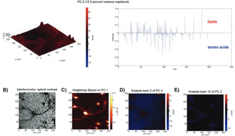
phosphocholine-containing phospholipids and a common marker for cell membranes in ToF-SIMS analysis.9,18Its frag-ment ions atm/z166, 104, 86 and 58 are also present in the loadings.9The negative loadings of PC2 contain peaks that are commonly associated with amino acids19such asm/z84 (Lys), 100 (Arg), 110 (His), 120 (Phe) and 130 (Trp). Based on the loadings, it appears that PC2 distinguishes between the cell membrane and the cytoplasm. This supposition is strength-ened by the scores plots in Fig. 3D and E that show positive scores at the top of the cells (2ndanalysis layer) and negative scores inside the cell material (15th analysis layer). The pres-ence of the ion atm/z184 only persists in the top two analysis layers, indicating that, with the given depth resolution, they originate from a 16–32 nm layer on the surface of the cell, which corresponds, with an order of magnitude, to the 8–10 nm thickness of a neuronal cell membrane.20In contrast, ion fragments associated with amino acids can be detected over all subsequent analysis layers in areas coinciding with the location of cells, indicating that they originate from the cyto-plasm. The negative scores of the background (areas not occu-pied by cells) in the scores plot of analysis layer 2 are

attributed to the extracellular matrix, which is supported by the disappearance of these fragments from the surrounding material in deeper analysis layers that subsequently display a score of zero, because neither lipids not amino acids are present in the glass substrate. Notably, if single ions such as m/z 184 or m/z 130 are used instead of the principal com-ponents, the cell features are not clearly visible due to the low SNR.

The method reported here presents the first time PCA has been performed on large scale (256 × 256 × 160 pixels) 3D ToF-SIMS images. This was made possible by first calculating the PCA loadings using a smaller subset of randomly selected pixels as a training set that could then be applied to the full data set to generate the scores images. The method has been validated using a well-defined 3D ToF-SIMS data set of a PS– PVP multilayer system before being applied to a 3D ToF-SIMS image of a neuronal network. The results clearly show that PCA separates the diﬀerent chemistries in its loadings and pro-vides information on spatial chemical distribution via the scores. Furthermore, the scores images have a 1.7–2.4 times better signal-to-noise ratio than can be obtained with single

Fig. 3 PCA of the neuronal cell network. (A) PC2 explains 15.5% of the variance: 3D scores image (left) and loadings plot (right). The positive load-ings of PC2 correspond to fragments associated with lipids and the negative loadload-ings correspond to fragments associated with amino acids. (B) Optical image obtained from the interferometer. (C) Heightmap based on the scores for PC1 (48.8% variance explained). The interface is deﬁned as scores = 0 and taken as a reference for the substrate plane. Scaling is performed using a maximum height of 2.5 µm (based on interferometry data) and assuming a constant sputter rate. The 3D scores image in A is z-corrected with this surface topography. (D) The PC2 scores plot for analysis layer 2 shows red pixels with positive scores (lipids) in areas where cells are present and blue pixels with negative scores (amino acids) in areas without cells. (E) The PC2 scores plot for analysis layer 15 shows blue pixels with negative scores (amino acids) in areas where cells are present and black pixels with scores equal to zero (substrate) in areas without cells.

[image:5.595.60.533.68.342.2]

(6)

ions. The depth resolution of the scores images does not diﬀer from that of the single ion images. In addition, the PCA scores can be used to correct z-oﬀsets due to the cells’topography. Importantly, our approach now makes 3D SIMS image proces-sing of biological samples with multivariate analysis accessible on a routine basis and considerably facilitates data analysis.

Acknowledgements

The authors thank the Engineering and Physical Sciences Research Council (EPSRC; EP/H022112/1) for financial support. We also thank Dhruma Thakker for the cell plating and Noreen Boyle for advice on cell preparation as well as Morgan Alexander, Bonnie Tyler and Wouter Zwysen for useful discussions about data analysis and presentation.

References

1 A. Adriaens, L. Van Vaeck and F. Adams, Mass Spectrom. Rev., 1999,18, 48.

2 M. Piggott and M. Zelzer, Chim. Oggi Chem. Today, 2014,

32, 5.

3 J. Brison, M. A. Robinson, D. S. Benoit, S. Muramoto, P. S. Stayton and D. G. Castner, Anal. Chem., 2013, 85, 10869.

4 M. K. Passarelli, C. J. Newman, P. S. Marshall, A. West, I. S. Gilmore, J. Bunch, M. R. Alexander and C. T. Dollery, Anal. Chem., 2015,87(13), 6696–6702.

5 I. S. Gilmore,J. Vac. Sci. Technol., A, 2013,31, 050819.

6 J. S. Fletcher, J. C. Vickerman and N. Winograd,Curr. Opin. Chem. Biol., 2011,15, 733.

7 Y. Vercammen, N. Moons, S. Van Nuﬀel, L. Beenaerts and L. Van Vaeck,Appl. Surf. Sci., 2013,284, 354.

8 B. J. Tyler, G. Rayal and D. G. Castner,Biomaterials, 2007,

28, 2412.

9 J. S. Fletcher, S. Rabbani, A. Henderson, N. P. Lockyer and J. C. Vickerman, Rapid Commun. Mass Spectrom., 2011,25, 925.

10 P. J. Cumpson, N. Sano, I. W. Fletcher, J. F. Portoles, M. Bravo-Sanchez and A. J. Barlow, Surf. Interface Anal., 2015,47, 986.

11 J. Bailey, R. Havelund, A. G. Shard, I. S. Gilmore, M. R. Alexander, J. S. Sharp and D. J. Scurr, ACS Appl. Mater. Interfaces, 2015,7, 2654.

12 D. J. Graham, M. S. Wagner and D. G. Castner,Appl. Surf. Sci., 2006,252, 6860.

13 S. Hofmann,Surf. Interface Anal., 1999,27, 825.

14 M. S. Wagner, D. J. Graham, B. D. Ratner and D. G. Castner,Surf. Sci., 2004,570, 78.

15 J. Malm, D. Giannaras, M. O. Riehle, N. Gadegaard and P. Sjövall,Anal. Chem., 2009,81, 7197.

16 D. Breitenstein, C. E. Rommel, R. Möllers, J. Wegener and B. Hagenhoﬀ,Angew. Chem., Int. Ed., 2007,46, 5332. 17 M. A. Robinson, D. J. Graham and D. G. Castner, Anal.

Chem., 2012,84, 4880.

18 M. K. Passarelli and N. Winograd, Biochim. Biophys. Acta, Mol. Cell Biol. Lipids, 2011,1811, 976.

19 M. S. Wagner and D. G. Castner,Langmuir, 2001,17, 4649. 20 L. J. Gentet, G. J. Stuart and J. D. Clements, Biophys. J.,

2000,79, 314.