Stochastic service network design with rerouting

Stochastic Service Network Design with Rerouting

Ruibin Baia∗_{, Stein W. Wallace}b_{, Jingpeng Li}d_{, Alain Yee-Loong Chong}c a_{Division of Computer Science, University of Nottingham Ningbo China,}

Ningbo, 315100, China. Tel: +86 574 88180278. [email protected].

b_{Department of Business and Management Science, Norwegian School of Economics,} NO-5045, Bergen, Norway. [email protected]

c_{Nottingham University Business School China, University of Nottingham Ningbo China.} [email protected]

d_{Department of Computer Science and Mathematics, University of Stirling, Stirling} FK9 4LA, UK. [email protected]

Abstract

Service network design under uncertainty is fundamentally crucial for all freight transportation companies. The main challenge is to strike a balance between two conflicting objectives: low network setup costs and low expected operational costs. Together these have a significant impact on the quality of freight services. Increasing redundancy at crucial network links is a common way to improve network flexibility. However, in a highly uncertain environment, a single predefined network is unlikely to suit all possible future scenarios, unless it is prohibitively costly. Hence, rescheduling is often an effective alternative. In this paper, we proposed a new stochastic freight service network design model with vehicle rerouting options. The pro-posed model explicitly introduces a set of integer variables for vehicle rerouting in the second stage of the stochastic program. Although computationally more expensive, the resultant model provides more options (i.e. rerouting) and flexibility for planners to deal with uncertainties more effectively. The new model was tested on a set of instances adapted from the literature and its performance and characteristics are studied through both comparative studies and detailed analyses at the solution structure level. Implications for practical applications are discussed and further research directions are also provided.

Keywords: Service network design; Stochastic programming; Transportation Logistics; Rerouting;

1. Background and Motivation

efficiently, the service network design problem has proven to be one of the most difficult combinatorial optimisation problems around (Crainic and Kim, 2007). Solving real-life problem instances to optimality is generally not possible. Opportunities to develop practical decision support systems for this problem have been strengthened by the latest advances in high performance computing and hybrid optimisation techniques. This has led to increased research attention in service network design in the past decade. Detailed reviews of such research efforts can be found in Christiansen et al. (2007) for maritime transportation, Crainic (2003) for long-haul transportation and Crainic and Kim (2007) for intermodal transportation. Most research cited in these reviews is concerned with models and solution methods for deterministic cases. However, freight services are subject to various uncertainties (in terms of demands, travel time, vehicle breakdowns, etc.) and their estimation by mean values is incapable of capturing the nature of the real-world problems.

Indeed, handling uncertainties in demand for freight transportation has become one of the most chal-lenging problems for freight forwarding companies. Previously, freight service companies was faced with challenges of satisfying fluctuating demands with cyclic patterns. According to one of the largest Chinese parcel express delivery companies, Shentong Express, back in 2009 freight transportation demand often peaked during the weekdays and fell drastically during the weekends. This was because of the fact that their major transportation demands were production supply chain related and there are more business engage-ments during weekdays than weekends. However, in the past 5 years or so, e-commerce, online shopping, and recent mobile commerce have truly transformed the landscape and expanded the scale of the freight transportation market. In 2012, Amazon recorded USD 61 billion in sales, a 27.1% increase from 2011. Fuelled by massive sales, the Chinese online shopping site, Taobao, secured more than USD 3 billion in sales on a single day on November 11, 2012, generating 80 million delivery requests which were simply too much for logistic companies to handle. The total online shopping sales in 2012 in China were estimated to be USD 1.3 trillion, up 27.9% from 2011 while the total number of deliveries is estimated to be 6 billion (CECRC, 2013). The diversities and uncertainties of online shoppers (in terms of their physical locations, shopping time, and types and quantities of items that they buy) have made freight service network design extremely difficult. Scientific research is badly needed to address the problem more efficiently.

over all scenarios. The problem was solved by a two-stage stochastic programming approach in which the master problem (or the first-stage problem) was the determination of a cost-effective service network. The second-stage problem was to find, for a given demand realisation, a cost-minimal flow based on the network obtained in the first stage and outsourcing. The second stage problem serves as a feedback mechanism to the master problem to achieve a balance between the degree of redundancy in network capacity, the network’s structure, and the amount of outsourcing (which is often very expensive and strategically unpopular for freight companies). The experiments on a large number of small problem instances showed that stochastic service network design could potentially reduce the costs substantially compared with the solution obtained by a deterministic model. Several interesting patterns have been observed from the experiments, which have profound implications for service network design. A limitation of the model is that the only alternative to using the service network established in the first stage is outsourcing. In practice, a freighter could also re-adjust this network based on observed values of the uncertainties. Hoff et al. (2010) is the continuation of Lium et al. (2009), with the primary aim of developing efficient approaches that can solve large real-sized instances. A Variable Neighbourhood Search (VNS) based approach was proposed and its performance was evaluated on a set of instances of large sizes, which, according to Hoff et al. (2010), is promising.

Our research paper extends the work done in Lium et al. (2009) by incorporating rerouting as a second means of achieving flexibility. This was motivated by the fact that rerouting is a popular means used by freighters to adapt to unforeseeable changes and uncertainties. Compared with outsourcing, rerouting is favourable for freighters in terms of service quality control and long term development strategies. It is not in a freighter’s long-term interest to outsource large amounts of demand to its competitors. Additionally, we are also interested in investigating: 1) in what way rerouting will lead to a different network compared with the deterministic network and the network obtained through Lium et al. (2009)’s stochastic model; 2) how the nature of demand stochasticity will affect the performance of different models.

The main contribution of this paper is two-fold: primarily, we propose a stochastic programming model for stochastic service network design with options of both vehicle rerouting and service outsourcing to address demand stochasticity more efficiently. Secondly, some interesting observations and insights drawn from our experimental studies could have important implications for stochastic service network design practices. Application of the proposed model could potentially substantially reduce network setup costs and expensive outsourcing, but maintain a similar level of flexibility to those that can be offered by other related models in the literature.

and its effect on operational flexibility. It is also worth noting that for many applications that fit into this modelling scheme, particularly trucking, but also air airfreight transportation, data is normally available in large amounts, and estimating distributions is not unreasonable.

As for earlier papers, we have formulated our model in a two-stage setting. This is not primarily for simplicity, but because we see this as the most appropriate framework. The problem we are discussing in this paper is what has been called an “inherently two-stage problem”, see Chapter 1 of King and Wallace (2012). These are problems where the first stage is structurally different from all the others. In our case the first stage is to set up the service network, the rest amount to using/operating the network from Stage 1 in an uncertain environment. Typically, the first stage decisions are either expensive or irreversible (or both). For such models, the focus is on Stage 1, all the other stages are there only for creating a correct understanding of how the network will be operated, so as to get the network set up correctly. The clue of such models is the flow of information from the operational phase to the design phase. It is important to realise that the later stages are not interesting in their own rights; It is quite clear that once the service network is established, a much more detailed model will be developed for operational decisions. So the quality of how we model the operational phase should be based on its ability to feed back to the Stage 1 decisions, and not on its ”accuracy”. In this regard we are also following earlier work, such as Lium et al. (2009). So although the use of the service network in principle is an infinite horizon problem (or maybe just one with a very large but finite number of stages) representing the life of the design, we represent it with weekly snap-shots (scenarios) of demand patterns. For each scenario we model the transportation, including rerouting (and route recovery) of vessels and outsourcing of goods. This is of course an approximation (like all models are), but describes well the setting in which the service network must operate. So for this kind of models, it is actually a goal to avoid the multi-stage aspect of the real problem. That contains a lot of details which are not needed for setting up the network. Only when we reach the operational phase itself do we need to care about the small details related to the fact that the operations take place in a dynamic environment.

2. Literature Review

frequency and delivery timetables), the flow distribution paths for each commodity, the consolidation poli-cies, and the idle vehicle re-positioning, so that legal, social, and technical requirements are met (Wieberneit, 2008). This section aims to provide a brief overview of service network design only. More comprehensive reviews can be found in Crainic (2000); Crainic and Kim (2007) and Wieberneit (2008).

The research mentioned above has primarily been concentrating on problems of a static, deterministic nature. However, service network planning involves several uncertain aspects, such as unpredictable demands, traffic congestion, delays, and vehicle breakdowns. Optimal solutions for a deterministic problem may turn out to have poor quality or even lose feasibility as a result of uncertain factors (the latter does not happen in this paper, though). Therefore, uncertainty (particularly uncertain demands) in freight transportation is one of the most challenging issues that a freight company face every day. On one hand, the freighter wants to increase the revenue by servicing as much of the demand as possible. On the other hand, the freighter also wants to make sure that the provision of this service does not lead to a negative impact on profitability. There are a number of methods that a freighter can use to tackle the uncertain demand, including demand forecasting, real-time information gathering (demand, traffic, positioning), external vehicle hiring, vehicle rerouting, outsourcing, etc. Some forecasting methods lead to point forecasts (only), hence easily resulting in deterministic modelling in the design phase. This paper discusses what might happen in such cases. Alternatively, forecasting may be done in the form of demand distributions. The challenge is then how to use this information effectively, also a subject of this paper.

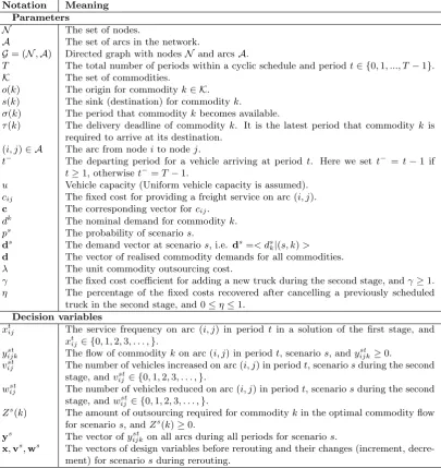
Table 1: List of notations used in the SNDP model

Notation Meaning Parameters

N The set of nodes.

A The set of arcs in the network.

G= (N,A) Directed graph with nodesN and arcsA.

T The total number of periods within a cyclic schedule and periodt∈ {0,1, ..., T−1}.

K The set of commodities.

o(k) The origin for commodityk∈ K.

s(k) The sink (destination) for commodityk.

σ(k) The period that commoditykbecomes available.

τ(k) The delivery deadline of commodityk. It is the latest period that commodityk is required to arrive at its destination.

(i, j)∈ A The arc from nodeito nodej.

t− The departing period for a vehicle arriving at periodt. Here we sett− = t−1 if t≥1, otherwiset−=T−1.

u Vehicle capacity (Uniform vehicle capacity is assumed). cij The fixed cost for providing a freight service on arc (i, j).

c The corresponding vector forcij.

dk The nominal demand for commodityk.

ps _{The probability of scenarios.}

ds The demand vector at scenarios, i.e. ds=< dsk|(s, k)>

d The vector of realised commodity demands for all commodities.

λ The unit commodity outsourcing cost.

γ The fixed cost coefficient for adding a new truck during the second stage, andγ≥1. η The percentage of the fixed costs recovered after cancelling a previously scheduled

truck in the second stage, and 0≤η≤1. Decision variables

xt

ij The service frequency on arc (i, j) in period t in a solution of the first stage, and

xtij∈ {0,1,2,3, . . . ,}.

yijkst The flow of commoditykon arc (i, j) in periodt, scenarios, andy st ijk≥0.

vst

ij The number of vehicles increased on arc (i, j) in periodt, scenariosduring the second

stage, andvijst∈ {0,1,2,3, . . . ,}.

wst

ij The number of vehicles reduced on arc (i, j) in periodt, scenariosduring the second

stage, andwstij∈ {0,1,2,3, . . . ,}.

Zs_{(k) The amount of outsourcing required for commoditykin the optimal commodity flow}

for scenarios, andZs(k)≥0.

ys _{The vector ofy}st

ijk on all arcs during all periods for scenarios.

x,vs,ws The vectors of design variables before rerouting and their changes (increment, decre-ment) for scenariosduring rerouting.

the uncertainties. Experiments and simulation data showed that the stochastic approach is more favourable than solutions produced by deterministic methods.

3. Problem Description and Formulation

The advantage of this time-space network model is its ability to integrate multi-class services (i.e. first-class, second class and deferred deliveries, etc.) into one model. Of course this comes at the cost of solving a large-scale network design model. It should be noted that the SNDP problem is different from the classical vehicle routing problem (VRP), in which nodes often represent end-customers. Rather, nodes in the SNDP correspond to freight centres (e.g. cities or regions), with each of them covering all nearby customers.

The notations used in this paper is given in Table 1. To develop our new stochastic model, we also present its deterministic counterpart and the stochastic model in Lium et al. (2009) for comparison.

3.1. The deterministic model (M-Determ)

We now present the basic deterministic service network design model used in Lium et al. (2009) with a few minor differences in notation and presentation.

M-Determ

min ∑

i∈N

∑

j∈N T_∑−1

t=0

cijxtij (1)

subject to

∑

j∈N

xt_ji− = ∑ j∈N

xt_ij ∀i,∀t (2)

∑

k∈K

y_ijkt ≤ uxt_ij ∀i,∀j,∀t,∀i̸=j (3)

−∑ j∈N

yt_jik− +∑ j∈N

y_ijkt =

          

dk if (i, t) is supply node fork −dk _{if (i, t) is demand node for k}

0 otherwise

∀i,∀t,∀k (4)

y_ijkτ(k) = 0 ∀i,∀j,∀k (5)

xt_ij ∈ Z+ ∀i,∀j,∀t (6)

y_ijkt ≥ 0 ∀i,∀j,∀t,∀k (7)

may take more than the planning horizon to reach its destination in order to take advantage of some cheap and unused truck capacities. This is due to the cyclic periods used in the model (i.e. the period afterT−1 is 0). Constraints (6) and (7) define feasible domains for the decision variables.

3.2. The Stochastic SNDP Model with Outsourcing

In this section we present Lium et al. (2009)’s two-stage stochastic model for service network design with uncertain demands, on which our proposed model is based. We use vector ds _{to denote all the demand} values of scenariosandps _{to stand for the probability of scenarios. In the first stage, a network is} deter-mined with the objective of minimising both the network setup cost and the expected additional costs to service demands across all scenarios. In the second stage, the model tries to find an optimal flow distribution between the predefined network from the first stage and the external network (via outsourcing). Decision variables, Zs_{(k), denote the amount of outsourcing required for commodityk in scenarios in the optimal} commodity flow. Note again that the presentation of the model is modified to keep it compact and in line with our own notation. Similar to constraints (5), constraints (14) are equivalents of constraints (19-21) and (23) in (Lium et al., 2009) to ensure that no commodity flow exists beyond its deadline. We denote this model asM-Stoch1for reference purposes in later sections.

M-Stoch1.

Stage 1:

min{cx+λ∑ s

psQ1(x,ds)} (8)

subject to

∑

j_∈N

xt_ji− = ∑ j_∈N

xt_ij ∀i,∀t (9)

xt_ij ∈ Z+ ∀i,∀j,∀t (10)

Stage 2:

Q1(x,ds) = min

∑

k∈K

Zs(k) (11)

∑

k∈K

yst_ijk ≤ uxt_ij ∀i,∀j,∀t,∀i̸=j (12)

−∑ j_∈N

y_jikst−+∑ j_∈N

yst_ijk =

          

dks−Zs(k) if (i, t) is supply node fork −dk

s+Zs(k) if (i, t) is demand node fork

0 otherwise

∀i,∀t,∀k (13)

y_ijksτ(k) = 0 ∀i,∀j,∀k (14)

yst_ijk ≥ 0 ∀i,∀j,∀k,∀t (15)

Zs(k) ≥ 0 ∀k (16)

In reality, this is of course not a two-stage problem. It has a large number of stages (possibly infinitely many), one for each period the design is being used. (Lium et al., 2009) chose a two-stage formulation, and we follow them. There are two reasons for this. Firstly, of course, it is for computational convenience; the model is certainly difficult enough with just two stages. But there is another important reason, namely that the focus of the model is the design, not the commodity flows themselves. The latter are needed in the model, as otherwise there would be no description of the purpose of the design. But the model is not meant to actually suggest flow patterns. The purpose of the second-stage is to feed back to the master problem the effects of different designs; it represents demand patterns that the network design must be able to handle. It is important that this feed-back is good, but it is not important that the second stage model itself produces possible ways of actually running the operations. As in (Lium et al., 2009) we believe that a two-stage model is sufficient to describe the use of the design in a good way.

3.3. The Proposed Stochastic Model

M-Stoch2

mincx+Q(x) (17)

subject to

∑

j∈N

xt_ji− = ∑ j∈N

xt_ij ∀i,∀t (18)

xt_ij ∈ Z+ ∀i,∀j,∀t (19)

where

Q(x) = ∑

s

psQ(x,ds) (20)

Q(x,ds) = min{γcvs−ηcws+λ∑ k∈K

Zs(k)} (21)

subject to

∑

j∈N

(v_jist−−w_jist−+xt_ji−) = ∑ j∈N

(vst_ij −w_ijst+xt_ij) ∀i,∀t (22)

∑

i∈N

∑

j∈N

(vst_ij−w_ijst) = 0 ∀t (23)

wst_ij ≤ xt_ij ∀i,∀j,∀t (24)

∑

k_∈K

y_ijkst ≤ u(v_ijst−wst_ij+x_ijt) ∀i,∀j,∀t,∀i̸=j (25)

−∑ j∈N

ystjik−+

∑

j∈N

yijkst =

           dk

s−Zs(k) if (i, t) is supply node fork −dk

s+Zs(k) if (i, t) is demand node fork

0 otherwise

∀i,∀t,∀k (26)

ysτ_ijk(k) = 0 ∀i,∀j,∀k (27)

v_ijst, wst_ij ∈ Z+ ∀i,∀j,∀t (28)

y_ijkst ≥ 0 ∀i,∀j,∀k,∀t (29)

Zs(k) ≥ 0 ∀k. (30)

the rerouting stage is more expensive than including it in the first stage (network design stage). Similarly, when a vehicle is cancelled in the rerouting stage, only a proportion of the cost (defined byη) is recovered. λ∑_k∈KZs_{(k) is the total cost to outsourceZ}s_{(k) demand where λis unit commodity outsourcing cost.}

Constraints (18) and (22) are the asset balancing constraints of the service network before and after rerouting. Constraints (23) make sure that for each period the total number of trucks remains the same before and after rerouting. Constraints (24) guarantee that we do not cancel more vehicles than we originally scheduled at any time. Constraints (25) make sure the vehicle capacity is respected. Constraints (26) are the commodity flow conservation constraints. Constraints (27) make sure that no flow exists after a commodity’s delivery deadline. Constraints (19) and (28) make sure design variables and rerouting offset variables are nonnegative integers, and constraints (29) and (30) ensure nonnegativity of commodity flow variables on both the internal service network and the external network.

In this model values of parameters γ andη can be set independently. It should be noted that, because of constraints (23), closing an arc at a given period will require to open another arc in the same period. Therefore, the actual rerouting cost (i.e. extra costs due to rerouting) consists of 100*(γ−1) percent of the setup cost of the new arc plus 100*(1−η) percent of the fixed cost of the cancelled arc. Here it is assumed that a vehicle, within the planning horizon, has a fixed standard route. Whenever a rerouting decision is made, a cost is incurred which is independent of rerouting frequency. The assumption is that for a company that has rerouting as a possible policy, rerouting is prepared for in such a way that rerouting costs do not change with frequency.

In order to have a better comparison with the stochastic model in Lium et al. (2009)’s research, we used the same uniform outsourcing cost coefficientλ. However, for practical applications, one possible extension of the model is to make this coefficient commodity dependent. For example, it could be more expensive to outsource hazardous goods or goods that have longer shipment distances. To do this, we could introduce λk _{as the cost of outsourcing one unit of commodityk. Without changing anything else or increasing the} computational complexity, we only need to change eq. (21) to the following:

Qs(x,ds) = min{γcvs−ηcws+∑ k∈K

λkZs(k)} (31)

Similarly, bothγandηcan be allowed to have an arc index if data is available. This does not change the computational burden of the models. But for a principal analysis like here, we believe that allowing these parameters to vary among routes will only confuse the numerical comparisons.

4. Solution Methodology

demand. Mostly we solve models using standard software (Cplex 12.4 MIP solver was used in this study). The main algorithmic contribution, which is more of an algorithmic setting than an actual implementation, is the analysis ofDeterm-Stoch2 andStoch1-Stoch2 (see sections 5 and 6). It turns out that these two heuristic settings have very interesting relationships to the true problem, M-Stoch2, and seem very efficient. This is something we shall follow up in later work.

Since the majority of previous research efforts for M-Determ and M-Stoch1 have been focusing on meta-heuristic approaches, for example tabu search (Pedersen et al., 2009) and guided local search (Bai et al., 2012) for Determ and variable neighbourhood search with fast approximations (Hoff et al., 2010) for M-Stoch1, we expect that similar approaches would also be suitable for M-Stoch2 although M-Stoch2 is much harder due to the additional rerouting variables.

There is also a collection of exact methods for stochastic integer programs where integrality appears in the second stage, see for example (Watson and Woodruff , 2011), (Watson et al. , 2012) and (Sen and Sherali, 2006). These can be bases for heuristics, the same way Crainic et al. (2011) used progressive hedging as a basis for a heuristic approach.

5. Experimental Setup

A number of experiments are set up to study the performance and solution characteristics of the three models (M-Determ, M-Stoch1 and M-Stoch2) that we presented in the previous section, and more impor-tantly, to find what this means for freight service planners. All three models could be solved directly for small instances. The results of the deterministic model (M-Determ) were obtained by solving it initially based on the nominal demands and then re-evaluating it in one of the stochastic models. More specifically, for each stochastic problem instance, M-Determ was firstly solved based on the average demand value (i.e. dk = 8), denoting the resulting solution byx. Then for each scenario sof the problem instance, we fix the networkx and then solve the flow distribution problem given by (11) of M-Stoch1. The objective value of M-Determ for this stochastic instance is the sum of the fixed cost ofxand the weighted average outsourcing costs among all scenarios (this could be computed according to Function (8)). The basic idea for this is to construct a service network based on the nominal demand data, and whenever a demand cannot be serviced in a particular scenario realisation (due to capacity constraints) it is outsourced according to M-Stoch1. For brevity, we denote this combination as Determ-Stoch1. Similarly, in the second stage the determin-istic solution could be re-evaluated in our proposed model M-Stoch2, and we denote this combination as

Determ-Stoch2. Finally, since M-Stoch2 is computationally more expensive than M-Stoch1 and is difficult

to solve directly, we also experimented with a third combination, denoted as Stoch1-Stoch2, where the initial network design is obtained via M-Stoch1 and the second stage problem is solved using M-Stoch2.

con-junction with IBM ILOG Cplex 12.4 MIP solver. All the experiments were run on a PC with 2.8GHz Intel i7 CPU, 4.0GB RAM, running Windows 7. The Cplex MIP procedure stops either when a maximum of 4-hour computational time is exhausted or the working memory exceeds 50GB.

Similarly to what was done in Lium et al. (2009), demand stochasticity was described by a combination of different levels of uncertainty and correlation types. Three correlation types were used to represent stochastic demands. Those are (a) all the demands positively correlated, (b) all uncorrelated, and (c) a mixture of positively and negatively correlated demand. Two triangular distributions (Tri(2,14,8) and Tri(5,11,8)) were used to simulate high and low uncertainties but with the same mean value (i.e. 8). We use the scenario generator by Høyland et al. (2003) and the methodology in Kaut and Wallace (2007) to ensure in-sample stability at a 5% level by determining the necessary number of scenarios.

It is important to see what we are doing here. All comparisons between models will be based on given scenario trees. Therefore, the optimal objective function value in M-Stoch2 is always (by construction) better than those of Determ-Stoch2 and Stoch1-Stoch2. No in-sample stability is needed for this to be the case. However, we have ensured in-sample stability (within 5%) in order to be sure that the problems we solve all represent reasonably well what we set out to solve (with given triangular marginal distributions and correlation matrices). Otherwise, the results are not easy to understand and interpret. With “wild” scenario trees, possibly representing very strange demand structures, the relationships among the alternative models may be very different from what would be the case with reasonable demand distributions (though M-Stoch2 would always be best).

Experiments were based on two sets of instances of different sizes, Set-LTL8 and Set-LTL20. Most instances in Set-LTL8 could be solved to optimality with regard to the different models discussed in Section 3. In this way, the optimal solutions obtained from these models could be analysed in a detailed manner and hopefully more insights could be gained during the process. For instances in Set-LTL20, M-Stoch2 generally cannot be solved optimally within our time limit. However, our main focus here is to understand uncertainty and rerouting, not to develop efficient heuristics.

Both sets contain instances with multiple sources and destinations. Set-LTL8 has 9 commodity sets adapted from Lium et al. (2009) 1 _{with slightly smaller sizes (we set the number of nodes |N | = 6, the}

number of periods T = 5, and the number of commodities in each set|K| = 8. Other parameters can be found from Table 2). Unless specified otherwise, these parameters will be used throughout the experiments in this paper. Combining different uncertainty levels and the types of correlations, this will result in 54 (= 9∗3∗2) instances in total, each of which has 20 demand scenarios. The second instance set, Set-LTL20, contains 8 randomly created commodity sets, each of which has 20 commodities (ie. |K|= 20). The scenario

Table 2: The parameters for the test problem instances in Set-LTL8.

parameters values fixed costs matrix (cij)

|N | 6 100 150 150 250 250 250 |K| 8 150 100 150 250 250 250

T 5 150 150 100 250 250 250

u 20 250 250 250 100 150 150

λ 150 250 250 250 150 100 150

γ 1.05 250 250 250 150 150 100

η 0.95

no. of scenarios 20

ps _1/20

profile was generated by using the high-level uncertainty distribution Tri(2,14,8) and a correlation matrix mixing both positives and negatives. All the other settings were the same as before. More details regarding this instance set will be described later in Section 6.1.

6. Computational Results Analysis

In this section we report the results and main findings from the experiments, with particular emphasis on how the new model performs in comparison with the other models. We are also interested in learning how rerouting and outsourcing will change the network design patterns obtained from the deterministic model as well as how they differ from each other. It is hoped that these analyses will provide insights for constructing heuristics for large instances where optimal solutions may not be available. For the sake of presentation, we use ni to denote the ith node in the physical network and nitto denote the ith node at period t in the time-space network. For example, n34 stands for the node 3 at period 4.

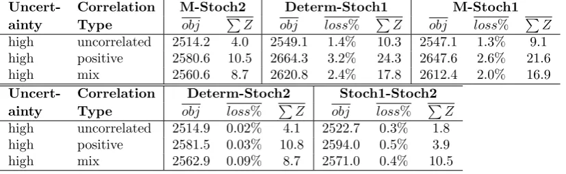
Table 3: A comparison of results between M-Determ, M-Stoch1 and our proposed model, M-Stoch2 over the small instance set Set-LTL8. For three commodity sets, Cplex failed to solve M-Stoch2 to optimality. The results for these three commodity sets are omitted from the statistics. obj(respectively∑Z) is the average objective (respectively total outsourcing averaged over all instances in each category) of the optimal solution from a given model for each particular problem category andloss% is the average relative losses by each method in comparison to M-Stoch2. Results for low-uncertainty scenarios are excluded due to very small differences between these models.

Uncert- Correlation M-Stoch2 Determ-Stoch1 M-Stoch1

ainty Type obj ∑Z obj loss% ∑Z obj loss% ∑Z

high uncorrelated 2514.2 4.0 2549.1 1.4% 10.3 2547.1 1.3% 9.1

high positive 2580.6 10.5 2664.3 3.2% 24.3 2647.6 2.6% 21.6

high mix 2560.6 8.7 2620.8 2.4% 17.8 2612.4 2.0% 16.9

Uncert- Correlation Determ-Stoch2 Stoch1-Stoch2

ainty Type obj loss% ∑Z obj loss% ∑Z

high uncorrelated 2514.9 0.02% 4.1 2522.7 0.3% 1.8

high positive 2581.5 0.03% 10.8 2594.0 0.5% 3.9

6.1. A general comparison of different models

To evaluate the performance of the three different models, Determ-Stoch1, M-Stoch1 and M-Stoch2, we implemented and tested them initially on the data set Set-LTL8, which contains problem instances that are sufficiently small so that all three models can be solved to optimality within the limits of the computing resources in terms of both time and working memory space. The results are benchmarked against the optima from M-Stoch2 and measured in terms of losses (see Table 3). The values we are presenting here are direct extension of the Value of the Stochastic Solution (VSS) as defined in Birge (1982). It measures the expected gain from using a stochastic rather than deterministic model.

Low-level uncertainty cases are not included in this table because the instances are very small and results from all three models are very similar. It can be seen that for each of the correlation types, the potential relative losses (measured against M-Stoch2) by Determ-Stoch1 and M-Stoch1 range from 1.3% to 3.2% even for these small-sized instances. The potential benefit for adopting M-Stoch2 is greater for instances with correlated demands (both positive or mixed) than for those with uncorrelated demands, as indicated by their relatively better objective values. Finally, results also show that M-Stoch2 outsources less demand than both Determ-Stoch1 and M-Stoch1. This could be one of the most important advantages for the proposed model since freight companies always strive to increase their market share and it is not in their long-term interest to outsource a large amount of demand to their competitors.

One of the challenges for the adoption of M-Stoch2 in practice is its high computational cost even for small cases. For larger instances, we normally cannot reach optimality even when we increase the computing resources significantly. Therefore, development of efficient heuristic approaches becomes necessary. In this research, we investigated two approaches that are similar to widely used decomposition methods. The main idea is to heuristically decompose the original problem (M-Stoch2) into two sub-problems or stages, namely network design and rerouting. The network design can be approximated by either M-Determ or M-Stoch1 without taking into account rerouting. Both models are easier to solve than M-Stoch2. Once a network is determined, it can then be passed to M-Stoch2 for obtaining optimal rerouting schedules and flow distributions for different scenarios. We denote these two approaches Determ-Stoch2 and

Stoch1-Stoch2respectively. The results by both Determ-Stoch2 and Stoch1-Stoch2 are also given in Table 3. The

Table 4: The Cplex solution time of different approaches for Set-LTL8 (in seconds).

Correlation Determ-

Stoch1-Uncertainty Type M-Determ M-Stoch1 M-Stoch2 Stoch2 Stoch2

high uncorrelated 0.2 0.9 358.9 2.8 3.5

high positive 0.2 0.8 1006.8 3.0 3.0

high mix 0.2 1.2 1288.2 4.2 3.7

Average time 0.2 1.0 884.6 3.3 3.4

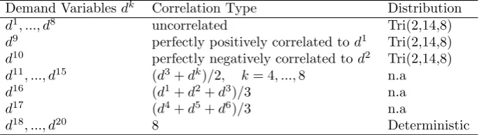
In order to further evaluate the performance of Determ-Stoch2 and Stoch1-Stoch2, we generated 8 larger instances (R1,...R8), each of which has 20 randomly generated commodities. The scenarios for these com-modities were generated by a mixture of uncorrelated random variables, perfectly correlated variables, linear combinations of random variables as well as deterministic ones (see Table 5 for details). Since there are only 8 independent random variables (d1_{, ..., d}8_{), we are able to reduce the number of scenarios to 13 while}

ensuring a low in-sample error (<5%).

Table 5: Parameters for the generation of a 20-commodity demand scenario file.

Demand Variablesdk _{Correlation Type Distribution}

d1_{, ..., d}8 _{uncorrelated Tri(2,14,8)}

d9 _{perfectly positively correlated tod}1 _Tri(2,14,8)

d10 _{perfectly negatively correlated tod}2 _Tri(2,14,8)

d11_{, ..., d}15 _(d3_+dk_{)/2, k= 4, ...,8 n.a}

d16 _(d1_+d2_+d3_{)/3 n.a}

d17 _(d4_+d5_+d6_{)/3 n.a}

d18, ..., d20 8 Deterministic

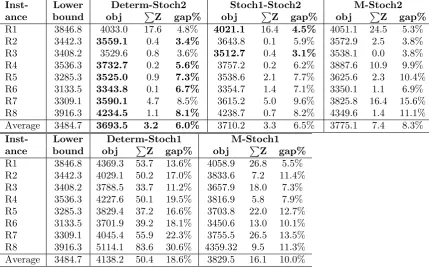
Table 6 presents the optimal solutions produced from the two decomposition approaches in comparison to the best results from M-Stoch2 which was not solved to optimality, and Table 7 gives the computational time spent by different approaches. In order to get an indication of the solution quality by the different approaches, the relative gaps (gap%) to a lower bound are also included in the table. Note that these lower bounds were obtained when attempting to solve M-Stoch2, and their quality may be poor when the solutions to M-Stoch2 are far from optimality. Therefore, a large relative gap to the lower bound does not necessarily imply a poor solution. However, a small relative gap indicates a good quality solution. From the table, it can be seen that with limited computing resources, M-Stoch2 returns some very poor solutions (e.g. R4, R5, R7 and R8) with gaps to the lower bound around 10% or even higher. In contrast, the two decomposition based heuristics performed much better, producing results better than M-Stoch2 for every instance while with less computational efforts.

Table 6: A comparison of the two decomposition heuristics and M-Stoch2 for dataset Set-LTL20 with maximum of 4 hours computing time and 50GB working memory. Both Determ-Stoch2 and Stoch1-Stoch2 were solved to optimality but M-Stoch2 failed to do so. Lower bounds were obtained while solving M-Stoch2. The best results are highlighted in bold. obj is the objective value of the solution returned by a given approach and∑Zis the total amount of outsourcing. gap%is the relative gap to the lower bound, i.e. gap%=[(obj-lower bound)/lower bound]×100%.

Inst- Lower Determ-Stoch2 Stoch1-Stoch2 M-Stoch2

ance bound obj ∑Z gap% obj ∑Z gap% obj ∑Z gap%

R1 3846.8 4033.0 17.6 4.8% 4021.1 16.4 4.5% 4051.1 24.5 5.3%

R2 3442.3 3559.1 0.4 3.4% 3643.8 0.1 5.9% 3572.9 2.5 3.8%

R3 3408.2 3529.6 0.8 3.6% 3512.7 0.4 3.1% 3538.1 0.0 3.8%

R4 3536.3 3732.7 0.2 5.6% 3757.2 0.2 6.2% 3887.6 10.9 9.9%

R5 3285.3 3525.0 0.9 7.3% 3538.6 2.1 7.7% 3625.6 2.3 10.4%

R6 3133.5 3343.8 0.1 6.7% 3354.7 1.4 7.1% 3350.1 1.1 6.9%

R7 3309.1 3590.1 4.7 8.5% 3615.2 5.0 9.6% 3825.8 16.4 15.6%

R8 3916.3 4234.5 1.1 8.1% 4238.7 0.7 8.2% 4349.6 1.4 11.1%

Average 3484.7 3693.5 3.2 6.0% 3710.2 3.3 6.5% 3775.1 7.4 8.3%

Inst- Lower Determ-Stoch1 M-Stoch1

ance bound obj ∑Z gap% obj ∑Z gap%

R1 3846.8 4369.3 53.7 13.6% 4058.9 26.8 5.5%

R2 3442.3 4029.1 50.2 17.0% 3833.6 7.2 11.4%

R3 3408.2 3788.5 33.7 11.2% 3657.9 18.0 7.3%

R4 3536.3 4227.6 50.1 19.5% 3816.9 5.8 7.9%

R5 3285.3 3829.4 37.2 16.6% 3703.8 22.0 12.7%

R6 3133.5 3701.9 39.2 18.1% 3450.6 13.0 10.1%

R7 3309.1 4045.4 55.9 22.3% 3755.5 26.5 13.5%

R8 3916.3 5114.1 83.6 30.6% 4359.32 9.5 11.3%

Average 3484.7 4138.2 50.4 18.6% 3829.5 16.1 10.0%

influenced by the cost ratio between outsourcing (λ) and rerouting (γ, η). More discussions will be made later in Section 6.3.

It is interesting to observe that when the rerouting cost is moderate (10%), although the deterministic solution evaluated in M-Stoch1 is very poor (on average 18.6% off the lower bound, see Table 6), its per-formance evaluated in M-Stoch2 is significantly better, only 6.0% off the lower bound. Similar observation can also be made from Table 3. This may suggest that when rerouting is available at a relatively low cost during the second stage of the stochastic program, the deterministic solution is not as bad as one might think. Using average estimations of demands is still a good strategy to configure the freight service network so long as the truck rerouting is efficient and flexible enough to keep the cost low. On the other hand, M-Stoch1 achieved low expected costs through extra investment in the service network to generate flexibility in commodity routing. With the presence of rerouting in the second stage of the stochastic program, solutions from M-Stoch1 may be too “conservative” in the sense that some of the extra network investments may not be necessary. This is confirmed by the relatively inferior results by Stoch1-Stoch2 for R2,R4,R5,R6,R7,R8 in comparison to Determ-Stoch2. These trends can be observed from both Table 3 and Table 6.

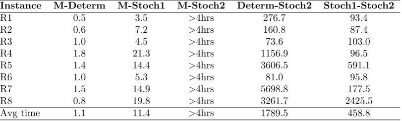
Table 7: The Cplex solution time of different approaches for Set-LTL20 (in seconds).

Instance M-Determ M-Stoch1 M-Stoch2 Determ-Stoch2 Stoch1-Stoch2

R1 0.5 3.5 >4hrs 276.7 93.4

R2 0.6 7.2 >4hrs 160.8 87.4

R3 1.0 4.5 >4hrs 73.6 103.0

R4 1.8 21.3 >4hrs 1156.9 96.5

R5 1.4 14.4 >4hrs 3606.5 591.1

R6 1.0 5.3 >4hrs 81.0 95.8

R7 1.5 14.9 >4hrs 5698.8 177.5

R8 0.8 19.8 >4hrs 3261.7 2425.5

Avg time 1.1 11.4 >4hrs 1789.5 458.8

Determ-Stoch2 did which is not surprising since the network from M-Stoch1 has more capacity. However, this is not always the case. For example, for instances R5, R6 and R7 in Table 6, and high uncertainty, mixed correlation instances in Table 3, Stoch1-Stoch2 actually outsourced more than Determ-Stoch2. The most likely reason for this is that though M-Stoch1 has higher installed capacity, the network structure is not very good. As can be seen from the example given in the next section, as well as the findings by Lium et al. (2009), that the network from M-Stoch1 is by no means a simple extension of the network from M-Determ. It involves fundamental network structural changes.

6.2. Structural differences between solutions from the three formulations

In this section we analyse differences in solution structures from the three models. To allow us to carry out a detailed study of the differences at solution level, we take a closer look at the solutions from the different models for an instance with highly uncertain demand. Instances with low demand uncertainties are not considered since the three formulations performed similarly for many of the small instances.

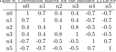
In this study, we experimented on a carefully generated new instance, denoted as LTL6-SW. It contains 12 nodes and 6 commodities shown in Figure 1.(a). The six grey-shaded nodes (numbered from 0 to 5) are source nodes of 6 commodities and node 11 is their common sink node. The rest of the nodes are purely consolidation/transhipment nodes. The values across the arcs represent the fixed costs of the corresponding arcs. Only arcs that are shown in the figure are considered in the network. The number of periods is set to 5. Therefore the network in Figure 1.(a) has a copy in each of the 5 periods. All 6 commodities, available at period 0, have to be delivered by period 4. The demands of the 6 commodities are drawn from a triangular distribution Tri(0,1,0.5) and the capacity of the truck is set to 1. Hence, on average, 1 truck can service two commodities. The correlation matrix used for scenario generation is given in Table 8. The costs for rerouting and outsourcing are set toγ= 1.125, η= 0.875, λ= 150.

Table 8: Correlation matrix for the instance LTL6-SW.

n0 n1 n2 n3 n4 n5

n0 1 0.7 0.4 0.4 -0.7 -0.7

n1 0.7 1 0.4 0.4 -0.7 -0.7

n2 0.4 0.4 1 0.8 -0.5 -0.5

n3 0.4 0.4 0.8 1 -0.5 -0.5

n4 -0.7 -0.7 -0.5 -0.5 1 0.7

n5 -0.7 -0.7 -0.5 -0.5 0.7 1

Table 9: Optimal truck routes according to different models for LTL6-SW.

M-Determ M-Stoch1 M-Stoch2

R1: 0→7→10→11→0 R1: 0→4→9→11→0 R1: 0→4→9→11→0 R2: 1→7→1 R2: 1→7→10→11→1 R2: 1→7→10→11→1 R3: 2→3→8→11→2 R3: 2→3→8→11→2 R3: 2→3→8→11→2 R4: 5→4→9→11→5 R4: 2→5→4→9→11→2 R4: 5→4→9→11→5

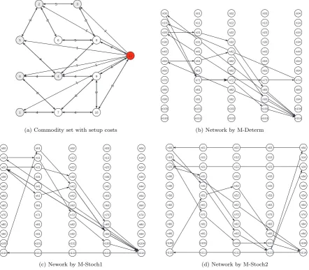
fixed cost of the network, M-Stoch1 is the most expensive one, due to an additional arc n2→n5 being used in route R4 in order to increase flexibility. The network from M-Determ lacks such flexibility in certain areas. An example is that the commodity from node 1 is consolidated at node 7, but only 1 truck departs from node 7 to node 11. On the other hand, in the networks from both M-Stoch1 and M-Stoch2, node 4 was used as a consolidation point for goods from node 0 and node 5. Since node 4 has two trucks going to node 11 and node 0 and node 4 have negatively correlated demand, this route provides flexibility. Regarding route R3 for commodities from nodes 2 and 3, which are positively correlated, there is also a lack of flexibility for three scenarios for all three networks. The solution from M-Stoch1 is to distribute some of the shipments of node 2 from route R3 to R4. In M-Stoch2, this was solved through rerouting at Stage 2, thereby transforming the network towards a network similar to that of M-Stoch1. That is, change R4 in M-Stoch2 to R4 in M-Stoch1 for these 3 scenarios. This observation is similar to the observation made in the previous example.

In general, we see that the deterministic solution pairs up commodities that turn out to be positively correlated. Hence, rerouting (or serious outsourcing) becomes necessary. The M-Stoch1 solution, though not knowing about rerouting, knows about the correlations and pairs things up differently. However, it may lead to a network that is over-conservative. The network created by M-Stoch2 lies between the networks from M-Determ and M-Stoch1 in such a way that its fixed costs are comparable to those of M-Determ, while the network is flexible and can easily and cheaply be transformed to the structure of the network from M-Stoch1 when handling some “extreme” scenarios.

6.3. Outsourcing versus rerouting

4

6

4 5

5 _{5 5}

4 ₆ 4 5 6 4 4 3 4 5 1 1 1 1 1 1 0 1 2 3 4 5 6 7 8 9 10 11

(a) Commodity set with setup costs

n00 n01 n02 n03 n04

n10 n11 n12 n13 n14

n20 n21 n22 n23 n24

n30 n31 n32 n33 n34

n40 n41 n42 n43 n44

n50 n51 n52 n53 n54

n60 n61 n62 n63 n64

n70 n71 n72 n73 n74

n80 n81 n82 n83 n84

n90 n91 n92 n93 n94

n100 n101 n102 n103 n104

n110 n111 n112 n113 n114

(b) Network by M-Determ

n00 n01 n02 n03 n04

n10 n11 n12 n13 n14

n20 n21 n22 n23 n24

n30 n31 n32 n33 n34

n40 n41 n42 n43 n44

n50 n51 n52 n53 n54

n60 n61 n62 n63 n64

n70 n71 n72 n73 n74

n80 n81 n82 n83 n84

n90 n91 n92 n93 n94

n100 n101 n102 n103 n104

n110 n111 n112 n113 n114

(c) Nework by M-Stoch1

n00 n01 n02 n03 n04

n10 n11 n12 n13 n14

n20 n21 n22 n23 n24

n30 n31 n32 n33 n34

n40 n41 n42 n43 n44

n50 n51 n52 n53 n54

n60 n61 n62 n63 n64

n70 n71 n72 n73 n74

n80 n81 n82 n83 n84

n90 n91 n92 n93 n94

n100 n101 n102 n103 n104

n110 n111 n112 n113 n114

(d) Network by M-Stoch2

Figure 1: Service networks by different models for a 12-node-6-commodity instance. Thick arcs mean more than 1 truck movement along the arc.

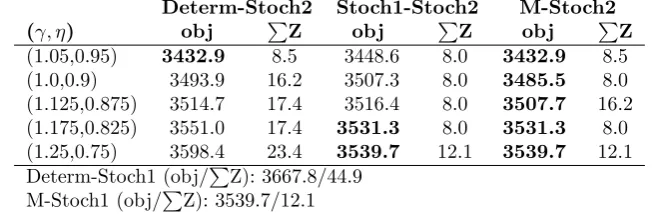
particularly when the rerouting cost is high. In fact, the relative ratio between the outsourcing cost and rerouting cost will have a major influence on the solutions produced by the different stochastic approaches. When the rerouting cost becomes much higher than outsourcing and fixed costs of the network, M-Stoch2 degenerates into Stoch1-Stoch2. On the other hand, when the rerouting cost is very low, it tends to lead to a same network as the one M-Determ obtains. Table 10 presents a comparison of different approaches with different rerouting costs for a 12-commodity-13-scenario instance that we adapted from one of instances in Set-LTL20 2_{. Five rerouting cost settings were used, ranging from 10% up to 50%. The results by}

Table 10: Performance of approaches at different rerouting costs for a 12-commodity-13-scenario instance.

Determ-Stoch2 Stoch1-Stoch2 M-Stoch2

(γ, η) obj ∑Z obj ∑Z obj ∑Z

(1.05,0.95) 3432.9 8.5 3448.6 8.0 3432.9 8.5

(1.0,0.9) 3493.9 16.2 3507.3 8.0 3485.5 8.0

(1.125,0.875) 3514.7 17.4 3516.4 8.0 3507.7 16.2

(1.175,0.825) 3551.0 17.4 3531.3 8.0 3531.3 8.0

(1.25,0.75) 3598.4 23.4 3539.7 12.1 3539.7 12.1

Determ-Stoch1 (obj/∑Z): 3667.8/44.9 M-Stoch1 (obj/∑Z): 3539.7/12.1

Determ-Stoch1 and M-Stoch1 are always the same since they do not operate with rerouting. It can be seen that for this instance when the rerouting cost is at 10%, M-Stoch2 has the same performance as Determ-Stoch2, suggesting that M-Stoch2 gives the same master network as the deterministic model. However, due to rerouting at the second stage of the stochastic program, it outsourced much less than Determ-Stoch1, and hence produced a better solution as far as the objective is concerned. M-Stoch2 performed best when the rerouting cost is at 20% or 25% but degenerated to Stoch1-Stoch2 when the rerouting cost reaches 35% or higher. At this rerouting cost level, M-Stoch1 outperformed Determ-Stoch2 but was inferior to Stoch1-Stoch2, suggesting its effectiveness even when the rerouting cost is very high. When the rerouting cost reaches 50%, M-Stoch2 converges to M-Stoch1, suggesting that rerouting did not come into play due to high costs and flexibility should be achieved through additional investments in the network.

6.4. Impact of commodity’s spatio-temporal distribution

It is not difficult to observe, from our previous experiments that highly uncertain demands are more difficult to handle, particularly for M-Determ and M-Stoch1. Better demand predictions are crucial for service network designs with good expected performance. Meanwhile, we have also observed that even with given demand scenario trees, a given model obtains solutions of considerably different objective values when the commodity sets are different. In other words, some commodity sets are far more expensive to service than others despite having the same commodity number and demand stochacity. From a freighter point of view, it is important to understand the characteristics (of a commodity set) that have led to this difference. With guidance of this knowledge, a freight company could then strategically develop/extend its current commodity set to maximise profitability. This prompted us to investigate the impact of different spatio-temporal distribution on the performance of the three models we discuss in this paper. It is hoped that, thorough a simple example, we could shed some light on this important issue. A thorough study regarding this topic is out of the main scope of this paper but will be our main research in future.

possibly. While the second commodity set (Figure 2.(b)) is made “clustered” in time dimension but with same physical departure and arrival nodes as those in the first commodity set. We did not change the physical departure/arrival nodes because the fixed costs of arcs are spatially dependent but they do not change over time. We used the same scenario matrices generated previously with a same nominal demand 8. The vehicle capacity is set to 10 for this particular experiment such that the network has innate (but limited) capacity redundancy to absorb uncertain demands. To maintain a similar ratio of fixed cost per unit vehicle capacity, arcs fixed costs are also halved here. All the other parameters remain the same as those in Table 2.

n00 n01 n02 n03 n04

n10 n11 n12 n13 n14

n20 n21 n22 n23 n24

n30 n31 n32 n33 n34

n40 n41 n42 n43 n44

n50 n51 n52 n53 n54

(a) A “balanced” commodity set

n00 n01 n02 n03 n04

n10 n11 n12 n13 n14

n20 n21 n22 n23 n24

n30 n31 n32 n33 n34

n40 n41 n42 n43 n44

n50 n51 n52 n53 n54

(b) A commodity set that is “clustered” in time

Figure 2: Two commodity sets with same origin/destination pairs but different departure and arrival times.

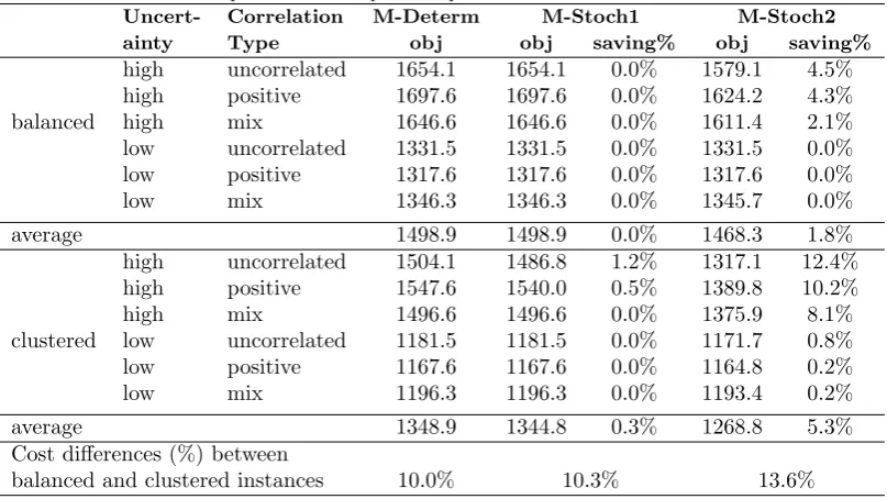
Table 11: The impact of demand spatio-temporal distribution on the service network.

Uncert- Correlation M-Determ M-Stoch1 M-Stoch2 ainty Type obj obj saving% obj saving%

high uncorrelated 1654.1 1654.1 0.0% 1579.1 4.5%

high positive 1697.6 1697.6 0.0% 1624.2 4.3%

balanced high mix 1646.6 1646.6 0.0% 1611.4 2.1%

low uncorrelated 1331.5 1331.5 0.0% 1331.5 0.0%

low positive 1317.6 1317.6 0.0% 1317.6 0.0%

low mix 1346.3 1346.3 0.0% 1345.7 0.0%

average 1498.9 1498.9 0.0% 1468.3 1.8%

high uncorrelated 1504.1 1486.8 1.2% 1317.1 12.4%

high positive 1547.6 1540.0 0.5% 1389.8 10.2%

high mix 1496.6 1496.6 0.0% 1375.9 8.1%

clustered low uncorrelated 1181.5 1181.5 0.0% 1171.7 0.8%

low positive 1167.6 1167.6 0.0% 1164.8 0.2%

low mix 1196.3 1196.3 0.0% 1193.4 0.2%

average 1348.9 1344.8 0.3% 1268.8 5.3%

Cost differences (%) between

balanced and clustered instances 10.0% 10.3% 13.6%

commodity sets. From the table it can be observed that high uncertainty (although with the same nominal values) will lead to higher network costs. When uncertainty is relatively low, the deterministic model is actually able to cope with most scenarios, mainly due to the difference between the capacity of the vehicles (10 in this experiment) and the nominal demands 8 in this experiment. It is particularly interesting to observe that when the commodities are clustered over time, the cost of the service network obtained by all three methods are much lower than the balanced solution. For these two particular instances, the difference in costs between a balanced commodity set and a clustered commodity set is at least 10% for all three models. This may be explained by the fact that when the commodities cluster well, there are more opportunities for consolidation and flow path sharing, both of which are beneficial for achieving flexibility, as found in Lium et al. (2009).

7. Conclusions and Future Research

Rescheduling is a widely adopted practice to deal with uncertainties. However, research on service network design with rerouting has not been looked at in the literature. In this work, we proposed a new stochastic freight service network design model with vehicle rerouting options. The model is an extension of a recent stochastic programming model (M-Stoch1) by Lium et al. (2009). In our model rerouting is explicitly modelled by a set of integer variables in the second stage of the stochastic programming model. Although computationally more expensive, the resultant model provides freight service planners with more flexibility to balance the conflict between the setup cost of the network and expected operational costs. In addition, it will allow freight companies to maximise their own transport capabilities optimally through rerouting and reduces outsourcing whenever possible. The model was tested on two sets of instances mainly drawn from the literature. Through both comparative studies and detailed analyses at the solution structure level, we made the following main observations and conclusions:

• Across all the test instances used in this paper with moderate rerouting costs, the proposed model M-Stoch2, when solved to optimality, is able to produce solutions with better objective values than M-Stoch1. More importantly, these solutions tend to use considerably less outsourcing than M-Stoch1, which is strategically important for the freight companies’ long-term ambitions.

• For large instances, M-Stoch2 is generally unsolvable. Decomposition-like heuristics in the forms of Determ-Stoch2 and Stoch1-Stoch2, however, produce better solutions than M-Stoch1 and M-Stoch2 do when the computational time is limited to 5 hours. These two heuristics could be used to develop efficient heuristic methods for M-Stoch2. The performance difference between Determ-Stoch2 and Stoch1-Stoch2 is very much dependent on the ratio between the outsourcing costs and rerouting costs.

• When demand is highly uncertain and correlated (both positive and mixed), the savings made using stochastic network design (M-Stoch1 and M-Stoch2) are among the highest. This does not come as a surprise since high-level, uncorrelated uncertainty is more expensive to handle. In a volatile market, freight companies should consider both the rerouting and outsourcing methods to leverage the risk and potential high costs resulting from demand uncertainty.

• It was found, through a numerical study, that the spatio-temporal distribution of demands could have a big impact on profitability. When demand (in terms of the size of the commodity set) is not high and is scattered evenly in the time-space network, both the deterministic model (M-Determ) and the stochastic models (M-Stoch1, M-Stoch2) generate solutions that are significantly more expensive (≥10% in our experiments) than the instances with “time-clustered” commodities. The implication for freight companies is to develop a market with certain beneficial spatio-temporal characteristics, which are not entirely explored yet but will be one of our future research directions.

Our future work will focus on the following two aspects. Firstly, we plan to make the model adoptable in practice by developing more efficient algorithms that are capable of solving large instances. Secondly, the model can be further extended by introducing other uncertainties in edge lengths and/or availabilities. Finally, it will be very interesting to understand better what constitute beneficial features in a commodity mix, in the sense that they lead to a good trade-off between initial design costs and expected operational costs (by using our model). Outcomes of this research would be extremely useful for freight companies to guide their market development/expansion. As far as we know, this research question has received very little attention so far in freight service network design literature.

Acknowledgements

Ahuja, R., Magnanti, T., Orlin, J., 1993. Network Flows: Theory, Algorithms and Applications. Prentice Hall.

Andersen, J., Christiansen, M., Crainic, T. G., Gronhaug, R., 2011. Branch and price for service network design with asset management constraints. Transportation Science 45 (1), 33–49.

Andersen, J., Crainic, T. G., Christiansen, M., 2009. Service network design with management and coordi-nation of multiple fleets. European Journal of Operational Research 193 (2), 377 – 389.

Armacost, A. P., Barnhart, C., Ware, K. A., 2002. Composite variable formulations for express shipment service network design. Transportation Science 36 (1), 1–20.

Bai, R., Kendall, G., Li, J., 2010. A guided local search approach for service network design problem with asset balancing. In: 2010 International Conference on Logistics Systems and Intelligent Management (ICLSIM 2010), January 9-10. Harbin, China, pp. 110–115.

Bai, R., Kendall, G., Qu, R., Atkin, J., 2012. Tabu assisted guided local search approaches for freight service network design. Information Sciences 189, 266–281.

Barnhart, C., Krishnan, N., Kim, D., Ware, K., 2002. Network design for express shipment delivery. Com-putational Optimization and Application 21 (3), 239–262.

Birge, J. R., 1982. The value of the stochastic solution in stochastic linear programs with fixed recourse. Mathematical Programming 24 (3), 314–325.

CECRC, 2013. 2012 China e-commerce market data monitoring report. url:

http://www.100ec.cn/zt/2012ndbg/.

Christiansen, M., Fagerholt, K., Nygreen, B., Ronen, D., 2007. Chapter 4 maritime transportation. In: Barnhart, C., Laporte, G. (Eds.), Handbooks in Operations Research and Management Science (Volume 14), 189–284.

Crainic, T., 2003. Long-haul freight transportation. Handbook of Transportation Science, 451–516.

Crainic, T. G., 2000. Service network design in freight transportation. European Journal of Operational Research 122 (2), 272 – 288.

Crainic, T. G., Fu, X., Gendreau, M., Rei, W. and Wallace, S. W., 2011. Progressive Hedging-based Meta-heuristics for Stochastic Network Design. Networks 58 (2), 114–124.

Crainic, T. G., Gendreau, M., Soriano, P., Toulouse, M., 1993. A tabu search procedure for multicommodity location/allocation with balancing requirements. Annals of Operations Research 41 (1-4), 359–383.

Crainic, T. G., Kim, K. H., 2007. Chapter 8 intermodal transportation. In: Barnhart, C., Laporte, G. (Eds.), Transportation. Handbooks in Operations Research and Management Science (Volume 14). Elsevier, pp. 467 – 537.

Crainic, T. G., Rousseau, J.-M., 1986. Multicommodity, multimode freight transportation: A general mod-eling and algorithmic framework for the service network design problem. Transportation Research Part B 20 (3), 225 – 242.

Crainic, T. G., Roy, J., 1988. Or tools for tactical freight transportation planning. European Journal of Operational Research 33 (3), 290 – 297.

Garrido, R. A., and Mahmassani, H. S., 2000. Forecasting freight transportation demand with the space-time multinomial probit model. Transportation Research Part B 34 (5): 403–418.

Ghamlouche, I., Crainic, T. G., Gendreau, M., 2003. Cycle-based neighbourhoods for fixed-charge capaci-tated multicommodity network design. Operations Research 51 (4), 655–667.

Ghamlouche, I., Crainic, T. G., Gendreau, M., 2004. Path relinking, cycle-based neighbourhoods and capac-itated multicommodity network design. Annals of Operations Research 131 (1-4), 109–133.

Hoff, A., Lium, A.-G., Løkketangen, A., Crainic, T., 2010. A metaheuristic for stochastic service network design. Journal of Heuristics 16 (5), 653–679.

Hu, Z., 2009. Personal Correspondance. Shentong Express Co., Ltd.

Høyland, K., Kaut, M., Wallace, S. W., 2003. A heuristic for moment-matching scenario generation. Com-putational Optimization and Applications 24 (2–3), 169–185.

Kaut, M., Wallace, S. W., 2007. Evaluation of scenario-generation methods for stochastic programming. Pacific Journal of Optimization 3 (2), 257–271.

Kim, D., Barnhart, C., Ware, K., Reinhardt, G., 1999. Multimodal express package delivery: a service network design application. Transportation Science 33 (4), 391–407.

Lin, B.-L., Wang, Z.-M., Ji, L.-J., Tian, Y.-M., Zhou, G.-Q., 2012. Optimizing the freight train connection service network of a large-scale rail system. Transportation Research Part B 46 (5), 649–667.

Lium, A.-G., Crainic, T., Wallace, S., 2009. A study of demand stochasticity in service network design. Transportation Science 43 (2), 144–157.

Nickel, S., Saldanha-da Gama, F., Ziegler, H.-P., 2012. A multi-stage stochastic supply network design problem with financial decisions and risk management. Omega 40 (5), 511–524.

Nourbakhsh, S. M., Ouyang, Y., 2012. A structured flexible transit system for low demand areas. Trans-portation Research Part B 46 (1), 204–216.

Pedersen, M. B., Crainic, T. G., Madsen, O. B., 2009. Models and tabu search metaheuristics for service network design with asset-balance requirements. Transportation Science 43 (4), 432–454.

Powell, W. B., 1986. A local improvement heuristic for the design of less-than-truckload motor carrier networks. Transportation Science 20 (4), 246–257.

Saboonchi, B., Zhang, G., 2010. A two-stage stochastic programming method for designing multi-stage global supply chains with stochastic demand. International Journal of Operational Research 9 (4), 409–425.

Sanchez-Rodrigues, V., Potter, A., and Naim, M. M., 2010. The impact of logistics uncertainty on sustainable transport operations, International Journal of Physical Distribution & Logistics Management 40: 61–83.

Sen, S. and Sherali, H. D., 2006. Decomposition with branch-and-cut approaches for two-stage stochastic mixed-integer programming. Mathematical Programming 106 (2), 203–223.

Shu, J., Teo, C.-P., Shen, Z.-J., 2005. Stochastic transportation-inventory network design problem. Opera-tions Research 53 (1), 48–60.

Szeto, W., Solayappan, M., Jiang, Y., 2011. Reliability-based transit assignment for congested stochastic transit networks. Computer-Aided Civil and Infrastructure Engineering 26 (4), 311–326.

Wang, D. Z. W., Lo, H. K., 2008. Multi-fleet ferry service network design with passenger preferences for differential services. Transportation Research Part B 42 (9), 798–822.

Watson, J.-P. and Woodruff, D. L., 2011. Progressive hedging innovations for a class of stochastic mixed-integer resource allocation problems. Computational Management Science 8 (4), 355–370.

Watson, J.-P., Woodruff, D. L. and Hart, W. E., 2012. PySP: modeling and solving stochastic programs in Python. Mathematical Programming Computation 4 (2), 109–149.