Discontinuous Galerkin methods for problems with Dirac delta source

Modélisation Mathématique et Analyse Numérique

DISCONTINUOUS GALERKIN METHODS FOR PROBLEMS WITH

DIRAC DELTA SOURCE

Paul Houston

_{and Thomas P. Wihler}

Abstract. In this article we study discontinuous Galerkin nite element discretizations of linear second-order elliptic partial dierential equations with Dirac delta right-hand side. In particular, assuming that the underlying computational mesh is quasi-uniform, we derive an a priori bound on the error measured in terms of theL2norm. Additionally,

we develop residualbased a posteriori error estimators that can be used within an adaptive mesh renement framework. Numerical examples for the symmetric interior penalty scheme are presented which conrm the theoretical results.

1991 Mathematics Subject Classication. 65N30.

June 17, 2011.

1. Introduction

In this article, we will consider the numerical approximation of the boundary value model problem

−∆u=δx0 inΩ, (1)

u= 0 on∂Ω, (2)

based on employing discontinuous Galerkin (DG) nite element discretizations. Here, Ω⊂R2 is an open bounded polygonal domain, and δx0 denotes the Dirac delta distribution at some given pointx0 ∈Ω. Throughout, in order to avoid technical diculties due to corner singularities, we

suppose that the domainΩis convex (this assumption can be relaxed in some parts of the article; this will be remarked on later). The weak formulation of (1)(2) is to ndu∈W₀1,p(Ω)such that

a(u, v) := Z

Ω

∇u· ∇vdx=v(x0) ∀v∈W01,q(Ω), (3)

with 1≤p <2, and 1 p+

1

q = 1. In this manuscript, for s∈N0 andt ≥1, W

s,t_{(Ω) signies the}

standard Sobolev space of all functions whose (weak) derivatives up to ordersare bounded in the Lt_{norm. Moreover, W}s,t

0 (Ω) is the subspace of functions belonging to Ws,t(Ω) with zero trace

along the boundary∂Ω. Ift= 2, we simply write Hs_{(Ω) =W}s,2_{(Ω). Following [3, Section 2] the}

above weak formulation is well-posed.

Keywords and phrases: Elliptic PDEs, discontinuous Galerkin methods, Dirac delta source.

∗_{Thomas Wihler acknowledges the nancial support of the Swiss National Science Foundation (SNF) under} grant No. 200021 126594

1 _{School of Mathematical Sciences, University of Nottingham, University Park, Nottingham, NG7 2RD, UK,} [email protected]

2_{Mathematics Institute, University of Bern, CH-3012 Bern, Switzerland, [email protected]}

c

Second-order elliptic partial dierential equations of the form (1)(2) are employed, for instance, in the modelling of diusion processes, heat ow, structural mechanics applications, or electric potentials, whenever point sources or loads occur. In addition, problems with a δ-source appear

as dual problems in deriving point-wise error estimates for nite element discretizations; see, e.g., [6, 10, 12]. From an analytical point of view, the challenge in describing such problems in a proper manner lies in the fact that the Dirac δ-distribution in R2 does not belong to H−1(Ω); thereby, the solution of (1)(2) is not anH1function. Consequently, the numerical approximation

of (1)(2) by, for example, nite element methods, requires a non-standard analysis. Here, in the context of conforming FEM, we mention the a priori results in [7, 17], as well as the a posteriori error analysis in [3]. For DG approximations to low-regularity problems, see, e.g., [13, 19].

The focus of the current paper is to extend some of the results developed for standard FEM to the context of discontinuous Galerkin methods. In particular, we shall derive a priori, as well as residual-based (global upper and local lower) a posteriori error estimates with respect to theL2

norm. Whilst striving to keep matters rather general, we will use the symmetric interior penalty discontinuous Galerkin method (SIPG), see [4, 9, 18], as an example to illustrate our results.

The outline of the article is as follows: In Section 2, we recall some basic denitions for dis-continuous Galerkin discretizations. Then, in Section 3 the a priori error analysis of a general class of DG methods on quasi-uniform meshes is presented. Section 4 presents the residualbased a posteriori error analysis. Subsequently, in Section 5 numerical experiments are undertaken to conrm the theoretical results. Finally, in Section 6 we add some concluding remarks.

2. Discontinuous Galerkin Methods

In this paper, we are interested in solving (1)(2) numerically by means of suitable discontinuous Galerkin discretizations. Before discussing these schemes, we will rst introduce a suitable nite element mesh framework for them.

2.1. Meshes, Spaces, and Element Boundary Operators

We consider shape-regular meshes T that partition Ω into open ane disjoint triangular or quadrilateral elements{K}K∈T, i.e.,Ω =SK∈T K. We suppose that T is constructed in such a manner thatx0 lies in the interior of some element K0∈ T. Furthermore, we permit meshes to

be 1-irregular. Each element K ∈ T is an image of the open reference triangle Tb ={(_bx1,x_b2) : −1 < x_b1 < 1,−1 < x_b2 < −x_b1} or of the open reference square Qb = (−1,1)2, respectively. By hK, we denote the diameter of an element K ∈ T; the elemental diameters are stored in a

vectorh= [hK]K∈T.

Moreover, we will dene some suitable element boundary operators that are required for DG methods. To this end, we denote by EI the set of all interior edges and by EB the set of all boundary edges inT. Additionally, we setE =EI∪ EB. The boundary ∂K of an element Kand the sets∂K\∂Ωand∂K∩∂Ωwill be identied in a natural way with the corresponding subsets ofE.

LetK] and K[ be two adjacent elements ofT, and xan arbitrary point on the interior edge

e∈ EI given bye=∂K]∩∂K[. Furthermore, letv andqbe scalar- and vector-valued functions,

respectively, that are suciently smooth inside each element K]/[. By(v]/[,q]/[), we denote the

traces of(v,q)onetaken from within the interior ofK]/[, respectively. Then, the averages of v

andq atx∈eare given by

hhvii= 1

2(v]+v[), hhqii= 1

2(q]+q[),

respectively. Similarly, the jumps ofvand qatx∈eare given by

respectively. Here, for K ∈ T, we denote bynK the unit outward normal vector to ∂K. On a

boundary edgee∈ EB, we sethhvii=v,hhqii=qand[[v]] =vn, withndenoting the unit outward

normal vector on the boundary∂Ω.

2.2. DG Discretizations

For a given nite element meshT and a xed polynomial degree`≥1, let us consider the DG nite element space

VDG(T) ={v∈L2(Ω) :v|K ∈S`(K)∀K∈ T }, (4)

where, for K ∈ T, S`(K) signies either the space P`(K) of all polynomials of total degree at

most`onK, when Kis a triangle, or the space Q`(K)of all polynomials of degree at most `in

each coordinate direction, whenKis a quadrilateral.

Let us now consider a DG bilinear formaDG(·,·)which discretizes the problem (1)(2), i.e., we

seek a DG solutionuDG∈VDG(T)such that

aDG(uDG, v) =v(x0) ∀v∈VDG(T). (5)

We assume that the matrix corresponding to aDG(·,·)on VDG(T)×VDG(T) is non-singular, so

that the discrete solutionuDG is uniquely dened. Moreover, we suppose that aDG(·,·)is of the

form

aDG(w, v) =

Z

Ω

∇hw· ∇hvdx+F(w, v), (6)

where∇hdenotes the elementwise gradient, andF(·,·)is a bilinear form featuring the numerical uxes of the DG scheme under consideration.

In order to give an example, we recall the symmetric interior penalty discontinuous Galerkin method (SIPG); see, e.g., [4, 5, 15, 18]. More precisely, for a xed parameterγ >0, we dene the DG form

aDG(w, v) =

Z

Ω

∇hw· ∇hvdx−

Z

E

hh∇hwii ·[[v]] ds

−

Z

E

[[w]]· hh∇hviids+γ

Z

E

h−1[[w]]·[[v]] ds.

(7)

Here,h∈L∞(E)is given by

h(x) = (

min(hK], hK[) forx∈∂K]∩∂K[∈ EI,

hK forx∈∂K∩∂Ω∈ EB.

For suciently largeγ >0, the formaDG(·,·)is coercive with respect to a suitable DG energy norm

and hence, using the SIPG form (7) in (5), the matrix corresponding to the bilinear formaDG(·,·)

is invertible; cf., e.g., [16].

3. Convergence Behavior on Quasi-Uniform Meshes

The aim of this section is to prove an a priori error estimate for the DG method (5) with respect to theL2_{norm. To this end, let us suppose that the meshT is quasi-uniform, with mesh}

sizeh:= maxK∈ThK, that is, there exists a constantρ >0such that

ρ < hK hK0

< ρ−1,

3.1. A Discrete

δ

-Function

Following the approach [17], we commence by constructing a discrete approximation δh ∈

VDG(T)of the Dirac delta functionδx0. More precisely, let

δh:=

(

0 onΩ\K0,

δK0 onK0,

whereK0∈ T is the unique element whichx0 belongs to. We deneδK0 ∈S`(K0)by Z

K0

δK0vdx=v(x0) ∀v∈S`(K0).

Clearly, we have that

Z

Ω

δhvdx=v(x0) (8)

for any v ∈ VDG(T). We now write Π`K0 to be the L

2_{projection operator onto}

S`(K0); more

precisely, givenw∈L2_(K

0), we dene Π`K0w∈S`(K0)as follows: Z

K0

(w−Π`<sub>K0</sub>w)vdx= 0 ∀v∈<sub>S</sub>`(K0). (9)

Thereby,

kδhkL2_(Ω)= sup v∈L2 (K0 )

v6≡0 Z

K0

δhvdx

kvk_L2_(K 0)

= sup v∈L2 (K0 )

v6≡0 Z

K0

δhΠ`K0vdx

kvk_L2_(K 0)

. (10)

Now, using thatkwk_L2_(K0)≥ Π`_K

0w _L2_(K

0)for anyw∈L

2_(K

0), we obtain

kδhkL2_(Ω)≤ sup v∈L2 (K0 )

Π` K₀v6≡0

Z

K0

δhΠ`K0vdx

Π`_K

0v

L2_(K 0)

= sup v∈L2 (K0 )

Π` K₀v6≡0

Π`_K

0v(x0)

Π`_K 0v

L2_(K 0)

≤ sup

v∈L2 (K0 ) Π`

K₀v6≡0 Π`_K

0v

L∞_(K0)

Π`_K

0v

L2_(K 0)

.

Furthermore, employing the inverse estimate

kwk_L∞_(K

0)≤Ch

−1

K0kwkL2(K0) ∀w∈S`(K0), (11) it follows that

kδhkL2_(Ω)≤Ch

−1

K0. (12)

In addition, lettingv≡1in (10) leads to

kδhk_L2_(Ω)≥

v(x0) kvk_L2_(K

0)

= 1

k1k_L2_(K 0)

≥Ch−_K1

0. (13)

3.2. A Priori Error Analysis

The functionδh from (8) is used to dene the ensuing auxiliary problem: −∆Uh=δh inΩ,

Uh= 0 on∂Ω.

The standard weak formulation is to ndUh∈H₀1(Ω) such that

a(Uh, v) = Z

Ω

Since Ω is convex, the Laplace operator ∆ : H2_(Ω)∩H1

0(Ω) → L2(Ω) is an isomorphism; see,

e.g., [8,11]. In particular,

∆−1

_L2_→H2_(Ω)∩H1 0(Ω)

<∞. (14)

Thus, we have

Uh

_H2_(Ω)≤CkδhkL2_(Ω). (15) Referring to [17], the following error bound holds

u−U

h

_L2_(Ω)≤Ch, (16)

whereuis the solution of (1)(2), andC >0is a constant depending on the distance ofx0to∂Ω.

In addition, using (8), we notice that the DG solutionuDG from (5) satises

aDG(uDG, v) =v(x0) =

Z

Ω

δhvdx

for anyv ∈VDG(T). Consequently,uDG can be seen to be the DG approximation ofUh. Hence,

provided that (14) holds, we may assume that we have the estimate

Uh−uDG

_L2_(Ω)≤Ch

2 Uh

_H2_(Ω). (17)

Indeed, this bound is true for various DG schemes in the literature (such as, for instance, the SIPG method (7)); see [5]. Thus, employing (12) we conclude that

Uh−uDG

_L2_(Ω)≤Ch

2_kδhk

L2(Ω)≤Ch. (18)

Thereby, exploiting the triangle inequality, gives

ku−uDGkL2_(Ω)≤ u−Uh

_L2_(Ω)+

Uh−uDG

_L2_(Ω); (19) inserting the bounds (16) and (18) into (19), we deduce the following result.

Theorem 3.1. Let T be a quasi-uniform mesh of mesh sizeh. Furthermore, suppose that (14),

as well as the L2_{error estimate (17) hold. Then, we have the following a priori error bound}

ku−uDGk_L2_(Ω)≤Ch,

where u and uDG are the solutions of (1)(2) and (5), respectively, and C > 0 is a constant

independent ofh.

Remark 3.2. We remark that the above error bound may be improved on meshes that are appropriately graded about the pointx0; see [2].

4. Residual-Based A Posteriori Error Analysis

We now proceed by developing an L2norm a posteriori error analysis of the DG schemes

dened in (5). Here, we derive both general upper and (local) lower bounds on the error measured in terms of theL2norm. Additionally, in order to present a specic example, the general results

4.1. Upper Bound

For anyp∈L2_{(Ω), let us consider the dual problem}

−∆ψ=p inΩ, (20)

ψ= 0 on∂Ω. (21)

The weak formulation reads: ndψ∈H1

0(Ω) such that

a(ψ, v) = Z

Ω

pvdx ∀v∈H01(Ω),

wherea(·,·)is the bilinear form dened in (3). By (14), we have the elliptic regularity estimate

kψk_H2_(Ω)≤Ckpk_L2_(Ω). (22)

For theL2_{norm of the erroru−u}

DG in the DG discretization, we may write

ku−uDGkL2_(Ω)= sup p∈L2 (Ω)

p6≡0 Z

Ω

(u−uDG)pdx

kpk_L2_(Ω)

. (23)

Here, for the integral we have Z

Ω

(u−uDG)pdx=a(u, ψ) +

Z

Ω

uDG∆ψdx=ψ(x0) +

Z

Ω

uDG∆ψdx.

Twofold integration by parts (element by element) of the last term results in Z

Ω

uDG∆ψdx = −

X

K∈T Z

K

∇uDG· ∇ψdx+

X

K∈T Z

∂K

(∇ψ·nK)uDGds

= X

K∈T Z

K

ψ∆uDGdx−

X

K∈T Z

∂K

(∇uDG·nK)ψds

+ X

K∈T Z

∂K

(∇ψ·nK)uDGds.

Furthermore, applying some elementary calculations, we obtain Z

Ω

uDG∆ψdx=

X

K∈T Z

K

ψ∆uDGdx−

Z

EI

[[∇huDG]]ψds+

Z

E

[[uDG]]· ∇ψds.

For anyψh∈VDG(T), there holds

ψh(x0) =aDG(uDG, ψh) =

Z

Ω

∇huDG· ∇hψhdx+F(uDG, ψh);

cf. (6). An elementwise integration by parts and elementary manipulations as before, yield that Z

Ω

∇huDG· ∇hψhdx

=− X K∈T

Z

K

ψh∆uDGdx+

X

K∈T Z

∂K

(∇uDG·nK)ψhds

=− X K∈T

Z

K

ψh∆uDGdx+

Z

E

hh∇huDGii ·[[ψh]] ds+

Z

EI

Therefore, we obtain that

Z

Ω

(u−uDG)pdx= (ψ−ψh)(x0) +

X

K∈T Z

K

(ψ−ψh)∆uDGdx

−

Z

EI

[[∇huDG]]hhψ−ψhiids+R[uDG, ψ](ψh),

where

R[uDG, ψ](ψh) =

Z

E

hh∇huDGii ·[[ψh]] ds+

Z

E

[[uDG]]· ∇ψds+F(uDG, ψh) (24)

is a residual term. We make the assumption that

|R[uDG, ψ](ψh)| ≤CΥ(uDG)|||ψ−ψh|||h, (25)

where C > 0 is a constant independent of h, Υ(uDG) is a computable quantity, and ||| · |||h is a

semi-norm such that we can nd an interpolantψh∈VDG(T)of the solutionψof (20)(21) with

h−_K2

0 sup

x∈K0

|(ψ−ψh)(x)| 2

+ X

K∈T

h−_K4kψ−ψhk2_L2_(K)

+ X

K∈T

h−_K2k∇(ψ−ψh)k 2

L2_(K)+|||ψ−ψh|||2h≤Ckψk 2 H2_(Ω),

(26)

for a constantC >0independent ofh. Here,K0∈ T is again the element containing the pointx0

which theδ-distributionδx0 from (1) is centered at. In order to proceed, we recall the L2_{projection onto}

S`(K0) from (9). Then, applying (8),

gives

(ψ−ψh)(x0) = (ψ−Π`K0ψ)(x0) + Π

`

K0(ψ−ψh)(x0)

= (ψ−Π`K0ψ)(x0) + Z

K0

Π`K0(ψ−ψh)δhdx

= (ψ−Π`_K0ψ)(x0) +

Z

K0

(ψ−ψh)δhdx.

Hence,

Z

Ω

(u−uDG)pdx= (ψ−Π`K0ψ)(x0) + X

K∈T Z

K

(ψ−ψh)(∆uDG+δh) dx

−

Z

EI

Therefore, using (25), it follows that Z Ω

(u−uDG)pdx

≤ sup

x∈K0

(Π`_K0ψ−ψ)(x) +

X

K∈T

kψ−ψhk_L2_(K)k∆uDG+δhk_L2_(K)

+ h

3

2[[∇_hu_DG]] _L2_(EI)

h

−3

2hhψ−ψ_hii

_L2_(EI)+CΥ(uDG)|||ψ−ψh|||h

≤C h2K0+ X

K∈T

h4Kk∆uDG+δhk 2 L2_(K)+

h

3

2_[[∇h_uDG]]

2

L2_(EI)+ Υ(uDG)

2

!12

×

h−_K2

0 sup

x∈K0

(ψ−Π`_K 0ψ)(x)

2

+ X

K∈T

h−_K4kψ−ψhk2_L2_(K)

+ h

−3

2hhψ−ψhii

2

L2_(EI)+|||ψ−ψh|||

2 h

12

.

Here, employing a standard trace inequality, we notice that

h

−3

2hhψ−ψ_hii

2

L2_(EI)≤C X

K∈T

h−_K3kψ−ψhk 2

L2_{(∂K\∂Ω)}

≤C X

K∈T

h−_K4kψ−ψhk2_L2_(K)+h−

2

K k∇(ψ−ψh)k 2 L2_(K)

.

Furthermore, sup

x∈K0

(ψ−Π`K0ψ)(x) ≤ sup

x∈K0

|(ψ−ψh)(x)|+ sup

x∈K0

Π`K0(ψ−ψh)(x) .

Applying the inverse estimate (11), leads to

sup

x∈K0

Π`_K0(ψ−ψh)(x)

≤Ch−_K1 0

Π`_K0(ψ−ψh)

_L2_(K0)≤Ch

−1

K0kψ−ψhkL2(K0).

It follows that Z Ω

(u−uDG)pdx

≤C h2_K0+ X

K∈T

h4_Kk∆uDG+δhk2_L2_(K)+ X

K∈T

h3_Kk[[∇huDG]]k2_L2_{(∂K\∂Ω)}+ Υ(uDG)2

!12

×

h−_K2

0 sup

x∈K0

|(ψ−ψh)(x)| 2

+ X

K∈T

h−_K4kψ−ψhk2_L2(K)

+ X

K∈T

h−_K2k∇(ψ−ψh)k 2

L2_(K)+|||ψ−ψh|||2_h 1₂

.

Recalling (26), this becomes

Z Ω

(u−uDG)pdx

≤C h2_K

0+ Υ(uDG)

2₊ X

K∈T e

ηK

!12

where, for eachK∈ T, the local error indicator_eηK is given by

e

ηK :=h4Kk∆uDG+δhk2_L2_(K)+h

3

Kk[[∇huDG]]k2_L2_{(∂K\∂Ω)}.

Thereby, for any constantκ >0, dening the error indicators ηκ,K:=h4Kk∆uDG+δhk

2

L2_(K)+h

3

Kk[[∇huDG]]k 2

L2_{(∂K\∂Ω)}+κ

2_h

Kk[[uDG]]k 2

L2_(∂K), (27) noting that [[u]]|E = 0 (for u ∈ W01,p(Ω)), employing the elliptic regularity bound (22), and

recalling (23), yields the following result.

Theorem 4.1. Let uDG be the DG solution given by (5) and ψ be the solution of (20)(21).

Assume that the residual R[uDG, ψ](ψh) dened in (24) satises (25) and (26) for some

semi-norm||| · |||h and some interpolantψh∈VDG(T). Then, the a posteriori error estimate holds

ku−uDGk2_L2_(Ω)+κ2 h

1

2_[[u−_uDG]]

2

L2_(E)≤C h

2

K0+ Υ(uDG)

2₊ X

K∈T

ηκ,K

!

, (28)

whereηκ,K,K∈ T, are the local error indicators dened in (27). The constantC >0 is

indepen-dent of handκ.

Remark 4.2. The two equivalent terms h

1

2[[u−u_DG]]

2

L2_(E)and P

K∈T hKk[[uDG]]k 2

L2_(∂K)have been added on both sides of the a posteriori error estimate (28) since the extendedL2_norm

ku−uDGk2

0,h≡ ku−uDGk 2

L2_(Ω)+κ

2

h 1

2[[u−u_DG]]

2

L2_(E)

of the error appears to be a suitable norm for proving local lower a posteriori error estimates; see the subsequent section.

4.2. Local Lower Estimates

Whilst our result in the previous section proves the reliability of the proposed a posteriori error estimator, we now focus on eciency bounds in the sequel. We note that the convexity of the domainΩis not required in this part of the article.

Let us consider the individual terms in the error indicatorηκ,K,K∈ T, from (27).

Proposition 4.3. For each K∈ T, the lower error bounds

k∆uDG+δhkL2_(K

0)≤Ch

−2

K0

kδh−δx0kH−2_(Ω)+ku−uDGk_L2_(K 0)

,

and

k∆uDG+δhkL2_(K)≤Ch

−2

K ku−uDGkL2_(K), K∈ T \ {K0},

hold.

Proof. For each elementK∈ T we dene a smooth bubble functionbK onK that satises

suppbK ⊆K, bK≥0, sup

x∈K

bK(x) = 1, bK|∂K= 0, ∇bK|∂K=0. (29)

Then, focusing on K0 rst and using the equivalence of norms in nite dimensional spaces, we

have that

Ck∆uDG+δhk 2 L2_(K

0)≤ Z

K0

v(∆uDG+δh) dx=

Z

Ω

(δh−δx0)vdx+ Z

K0

wherev:=bK(∆uDG+δh). Noticing that v|∂K0= 0 and

∇v|∂K₀ =bK|∂K₀∇(∆uDG+δh)|∂K0+∇bK|∂K0(∆uDG+δh)|∂K0=0,

integrating by parts twice in the second integral yields

Ck∆uDG+δhk 2 L2_(K

0)≤ Z

Ω

(δh−δx0)vdx+ Z

K0

∆v(uDG−u) dx

≤kδh−δx0kH−2(Ω)+ku−uDGkL2(K0)

kvk_H2(K0).

Again, due to equivalence of norms in nite dimensional spaces, and scaling, we have

kvk_H2_(K

0)≤Ch

−2

K0kvkL2(K0).

Hence,

Ck∆uDG+δhk 2

L2_(K0)≤h

−2

K0

kδh−δx0kH−2_(Ω)+ku−uDGkL2_(K0)

kvk_L2_(K0)

≤h−_K2

0

kδh−δx0kH−2_(Ω)+ku−uDGk_L2_(K0)

k∆uDG+δhk_L2_(K0).

Dividing both sides of the above inequality byk∆uDG+δhkL2_(K0)proves the proposition forK0.

ForK∈ T \ {K0}we letv=bK∆uDG and notice that δh|K = 0andv(x0) = 0. Thence,

Ck∆uDG+δhk 2

L2_(K)=Ck∆uDGk 2 L2_(K)≤

Z

K

v∆uDGdx=

Z

K

v∆(uDG−u) dx.

The remainder of the proof is very similar as before.

Proposition 4.4. OnK0, the following local lower bound holds

hK0 ≤C

ku−uDGk_L2(K0)+kδh−δx0kH−2(Ω)

.

Proof. On the elementK0consider a smooth bubble functionbK0 that satises the properties (29) as well as

bK0(x0) = 1, kbK0kL2_(K 0)≤

1 2kδhk

−1

L2_(K

0)=O(hK0), k∆bK0kL2_(K

0)≤Ch

−1

K0.

Due to (12) and (13), this construction is possible by choosing a bubble function possessing a suciently small support inK0. Then,

1 = Z

Ω

δx0bK0dx= Z

K0

∇(u−uDG)· ∇bK0dx+ Z

K0

∇uDG· ∇bK0dx.

Integration by parts, leads to

1 = −

Z

K0

(u−uDG)∆bK0dx− Z

K0

bK0∆uDGdx

= −

Z

K0

(u−uDG)∆bK0dx− Z

K0

(δh+ ∆uDG)bK0dx+ Z

K0

δhbK0dx

≤ ku−uDGkL2_(K0)k∆bK0kL2_(K0)+kδh+ ∆uDGkL2_(K0)kbK0kL2_(K0)

+kδhk_L2_(K

0)kbK0kL2(K0)

≤ Ch−_K1

This implies the bound

hK0≤C

ku−uDGk_L2_(K0)+h

2

K0kδh+ ∆uDGkL2_(K0)

.

Invoking the bound from Proposition 4.3 shows the estimate.

In order to bound the term k[[∇huDG]]kL2_{(∂K\∂Ω)} from (27) we assume that the mesh T is regular (i.e., it does not contain any hanging nodes).

Proposition 4.5. LetT be regular. Consider two elementsK], K[∈ T that share an interfacee=

(∂K]∩∂K[)◦∈ EI. We letωe:= (K]∪K[)◦. Then, the lower bound holds

h

3

2[[∇u_DG]]

_L2_(e)≤C

ku−uDGkL2_(ωe)+ h

1

2[[u−u_DG]]

_L2_(e)+kδh−δx0kH−2(Ω)

.

Proof. Following [13, 14], let us dene an auxiliary function χe∈H01(ωe)(which depends on the

function[[∇uDG]]|e) with the following properties:

χe|∂ωe = 0, ∇χe|∂ωe =0, [[∇χe]]|e= 0,

as well as

k[[∇uDG]]k 2

L2_(e)≤C Z

e

χe[[∇uDG]] ds,

and

h

−1

2∇χ_{e L2(e)}+

h−2χe

_L2_(ω

e)+kχekH2(ωe)≤C h

−3

2[[∇u_DG]]

_L2(e). (30) Then, we have

Ck[[∇uDG]]k2_L2_(e)≤ Z

e

χe[[∇uDG]] ds=

Z

∂K]

χe(∇uDG·nK]) ds+ Z

∂K[

χe(∇uDG·nK[) ds.

Applying Green's formula, we obtain

Ck[[∇uDG]]k 2

L2_(e) ≤ Z

ωe

∇χe· ∇huDGdx+

Z

ωe

χe∆huDGdx

= −

Z

ωe

∇χe· ∇h(u−uDG) dx+

Z

ωe

χe(∆huDG+δh) dx

−

Z

ωe

(δh−δx0)χedx,

where∆hsignies the elementwise Laplacian. Integrating by parts we get

−

Z

ωe

∇χe· ∇h(u−uDG) dx=−

Z

e

∇χe·[[u−uDG]] ds+

Z

ωe

(u−uDG)∆hχedx.

Thence,

k[[∇uDG]]k 2

L2_(e)≤C

h

−1

2∇χ_{e L}2_(e)

h

1

2[[u−u_DG]]

_L2_(e)+ku−uDGkL2(ωe)k∆hχekL2(ωe)

+kχek_L2_(ω

e)k∆huDG+δhkL2(ωe)+kδh−δx0kH−2(Ω)kχekH2(ωe)

Furthermore, we have

k[[∇uDG]]k2L2_(e)≤C

h

1

2[[u−u_DG]]

2

L2_(e)+ku−uDGk

2 L2_(ωe)+

h2(∆huDG+δh)

2 L2_(ω

e)

+kδh−δx0k

2 H−2_(Ω)

12

×

h

−1

2∇χ_e

2

L2_(e)+ h−2χe

2 L2_(ω

e)+kχek

2 H2_(ωe)

12

.

Using (30), and recalling the previous Proposition 4.3, it follows that

k[[∇uDG]]k2L2_(e)

≤C

h

1

2[[u−u_DG]]

2

L2_(e)+ku−uDGk

2 L2_(ω

e)+kδh−δx0k

2 H−2_(Ω)

12

kh−32[[∇u_DG]]kL2_(e).

Now, noting thath|ωe∼hK] ∼hK[, completes the proof. Finally, we have the identity

h

1 2_[[uDG]]

_L2_(∂K)= h

1

2_[[u−_uDG]]

_L2_(∂K), K∈ T, (31) by observing again that[[u]]|E = 0.

Remark 4.6. The termkδh−δx0kH−2_(Ω)appearing in the lower error estimates above takes the role of a data approximation term. We note that

Z

Ω

(δx0−δh)ψdx= (ψ−ψh)(x0)− Z

Ω

δh(ψ−ψh)

≤ sup

x∈K0

|(ψ−ψh)(x)|+kδhkL2_(K

0)kψ−ψhkL2(K0)

for anyψ∈H2(Ω)and anyψh∈VDG(T). Let us chooseψh∈S1(K),K∈ T, to be an interpolant

that satises the standard approximation estimate

h−_K2kψ−ψhk 2

L2_(K)+k∇(ψ−ψh)k 2

L2_(K)≤Ch

2 Kkψk

2

H2_(K), K∈ T. (32) Evidently, since∇2_ψ

h≡0on each element, we additionally have that

∇2(ψ−ψh)

_L2_(K)≤CkψkH2_(K), (33) where the constant C > 0 is independent of h. Furthermore, due to the continuous Sobolev

embeddingH2_(Ω),→L∞_{(Ω)(see, e.g., [1]), and by using a scaling argument, we conclude that} sup

x∈K

|(ψ−ψh)(x)| ≤ChKkψkH2_(K). (34)

Therefore, using the above bounds, together with (12), we obtain Z

Ω

(δx0−δh)ψdx≤ChK0kψkH2_(K 0)

for a constantC >0 independent ofh. Therefore,

kδx0−δhkH−2_(Ω)= sup

ψ∈H2_{(Ω),ψ6≡0} Z

Ω

(δx0−δh)ψdx

kψk_H2_(Ω)

4.3. Application to the SIPG method

We will now apply Theorem 4.1 to the SIPG method (7). More precisely, the quantityΥ(uDG)

from (25) will be dened explicitly. To this end, we start by noticing that the numerical uxes in the SIPG formaDG(·,·)from (7) satisfy

F(uDG, ψh) =−

Z

E

hh∇huDGii ·[[ψh]] ds−

Z

E

[[uDG]]· hh∇hψhiids+γ

Z

E

h−1[[uDG]]·[[ψh]] ds

for anyψh∈VDG(T). Consequently, the residualRfrom (24) satises

R[uDG, ψ](ψh) =

Z

E

[[uDG]]· hh∇h(ψ−ψh)iids+γ

Z

E

h−1[[uDG]]·[[ψh]] ds.

Using thatψ∈H1

0(Ω), we notice that[[ψ]] = 0onE. Therefore, we obtain |R[uDG, ψ](ψh)|

≤ Z E

[[uDG]]· hh∇h(ψ−ψh)iids

+ γ Z E

h−1[[uDG]]·[[ψ−ψh]] ds

≤ h 1 2[[u_DG]]

_L2_(E)

h

−1

2hh∇h(ψ−ψ_h)ii _L2_(E)+

γh

1 2[[u_DG]]

_L2_(E)

h

−3

2[[ψ−ψ_h]] _L2_(E).

Employing the Cauchy-Schwarz inequality, this implies (25), with

Υ(uDG) :=

p

1 +γ2 h

1 2[[u_DG]]

_L2_(E)≤C p

1 +γ2 X K∈T

h2_Kk[[uDG]]k 2 L2_(∂K)

!12

, (35)

and

|||ψ−ψh|||2h:=

h

−1

2hh∇_h(ψ−ψ_h)ii

2

L2_(E)+ h

−3

2[[ψ−ψ_h]]

2

L2_(E)

≤C X

K∈T

h−_K3kψ−ψhk2_L2_(∂K)+h−

1

K k∇(ψ−ψh)k 2 L2_(∂K)

.

Applying the trace inequality, with scaling, yields

|||ψ−ψh|||2 h≤C

X

K∈T

h−_K4kψ−ψhk2_L2_(K)+h

−2

K k∇(ψ−ψh)k 2 L2_(K)+

∇2(ψ−ψh)

2 L2_(K)

.

We choose ψh ∈VDG(T)to be an interpolant ofψ that fulls the bounds (32)(34); this then

implies that (26) holds.

Thus, employing Theorem 4.1 and recalling (35), we deduce the following result.

Theorem 4.7. The SIPG method (7) for the numerical approximation of (1)(2) satises the a posteriori error estimate

ku−uDGk2

L2_(Ω)+κ2 h

1

2_[[u−_uDG]]

2

L2_(E)≤C h

2 K0+

X

K∈T

ηSIPGκ,K

!

, (36)

where

ηκ,KSIPG:=h4Kk∆uDG+δhk 2

L2_(K)+h3Kk[[∇huDG]]k 2

L2_{(∂K\∂Ω)}+ (1 +γ2+κ2)h2Kk[[uDG]]k 2 L2_(∂K),

for any K ∈ T, and any constant κ >0. Here, C >0 is a constant independent of h, uDG,γ,

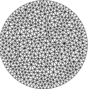
Figure 1. Initial mesh, consisting of 988 elements.

Remark 4.8. Local lower a posteriori error estimates for the SIPG scheme are given by the gener-ally valid estimates from Section 4.2. Evidently, a sensible choice ofκis given byκ∼γ. This will

ensure the equivalence of the termsκ2

h

1

2[[u−u_DG]]

2

L2_(E)and(1+γ

2_+κ2₎P

K∈Tk[[uDG]]k 2 L2_(∂K) appearing on the left and right-hand side of the a posteriori error estimate (36), respectively; cf. (31).

Remark 4.9. We note that the convexity of Ω is not essential in the a posteriori error analy-sis above. In the non-convex case, however, the presence of possible corner singularities in the solution ψ of (20)(21) implies that ψ ∈ W2,p_{(Ω) for some p < 2 rather than ψ ∈ H}2_{(Ω); see,}

e.g., [11]. Consequently, a rened analysis based onLp _{spaces is required. This can again be done}

along the lines of [3]; cf. also [19].

5. Numerical Examples

We consider the case when the computational domain Ωis the unit disc, i.e., Ω ={x∈ _R2 _: |x| < 1}. Settingx0 =0, the analytical solution to (1)(2) is the fundamental solution of the

Laplace equation; namely,

u(x) =− 1

2πln|x|.

Our numerical experiments are based on the SIPG method (7); here, we chooseγ =κ= 10. Firstly, we investigate the asymptotic convergence of the SIPG on a sequence of successively ner quasi-uniform unstructured triangular meshes for`= 1,2. Here, the initial mesh consists of 988 elements; cf. Figure 1. In Tables 1 and 2 we present a comparison of theL2_{(Ω)norm, as well as the}

extendedL2_{(Ω)norm dened in Remark 4.2, of the erroru−u}

DGfor`= 1,2, respectively, as the

initial mesh is uniformly rened. In each case we show the number of elements in the computational mesh, the number of degrees of freedom in the nite element space VDG(T), the corresponding

L2_{(Ω)norm and extendedL}2_{(Ω)norm of the error, together with their respective computed rate}

of convergencek. Here, we observe that (asymptotically)ku−uDGkL2_(Ω)converges to zero at the rateO(h)as htends to zero, cf. Theorem 3.1. Similar behavior of the normku−uDGk0,h is also

observed asymptotically.

Secondly, we now investigate the performance of the a posteriori error estimate derived in Theorem 4.7 within an automatic hversion adaptive renement procedure which is based on

1-irregular triangular elements, with`= 1. Thehadaptive meshes are constructed by marking the

Elements Dof ku−uDGkL2_(Ω) k ku−uDGk0,h k

988 2964 0.5096E-02 0.00 0.1019 0.00

3952 11856 0.3004E-02 0.76 0.4105E-01 1.31 15808 47424 0.2133E-02 0.49 0.1677E-01 1.29 63232 189696 0.8467E-03 1.33 0.9547E-02 0.81 252928 758784 0.5272E-03 0.68 0.4981E-02 0.94

Table 1. Convergence of ku−uDGkL2_(Ω) and ku−uDGk0,h on quasi-uniform triangular meshes with`= 1.

Elements Dof ku−uDGkL2_(Ω) k ku−uDGk0,h k

988 5928 0.2112E-02 0.00 0.1100 0.00

3952 23712 0.1451E-02 0.54 0.3400E-01 1.69 15808 94848 0.7444E-03 0.96 0.1715E-01 0.99 63232 379392 0.3484E-03 1.10 0.8688E-02 0.98 252928 1517568 0.1817E-03 0.94 0.6064E-02 0.52 Table 2. Convergence of ku−uDGkL2_(Ω) and ku−uDGk0,h on quasi-uniform triangular meshes with`= 2.

103 104 105 106

10−4 10−3 10−2 10−1 100

Error Bound True Error

Degrees of Freedom

0 2 4 6 8 10

0 1 2 3 4 5 6

E

ffe

ct

ivi

ty

Inde

x

Mesh Number

(a) (b)

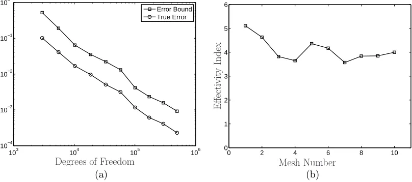
Figure 2. (a) Comparison of the actual and estimated extendedL2_{(Ω)norm of}

the error with respect to the number of degrees of freedom; (b) Eectivity indices.

actual and estimated extended L2_{(Ω)norm of the error on each of the meshes generated based}

on employing hadaptive mesh renement. Here, we observe that the a posteriori bound

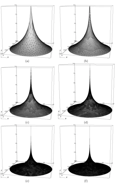
over-estimates the true error by a consistent factor. Indeed, the eectivity index tends to a value of around4as the mesh is adaptively rened, cf. Figure 2(b). In Figure 3 we plot the meshes overlayed onto the corresponding computed DG solution after 0 (initial mesh), 2, 4, 6, 8, and 9 adaptive renement steps have been undertaken. Here, we observe that the mesh has been signicantly rened in the vicinity of the origin of the computational domain, where the delta-source term is centered, as expected.

6. Conclusions

(a) (b)

(c) (d)

(e) (f)

partial dierential equations with Dirac delta right-hand side. In particular, the a priori bound indicates that theL2_{norm of the discretization error converges to zero at the rate O(h) as the}

mesh sizehtends to zero. Secondly, computable residualbased a posteriori error indicators have

been derived when the error is measured in terms of an extendedL2_{norm; the use of this norm}

facilitates the derivation of local lower bounds. These theoretical results have been conrmed numerically; in particular, the a posteriori error bound has been employed within an automatic adaptive mesh renement algorithm.

References

[2] T. Apel, O. Benedix, D. Sirch, and B. Vexler. A priori mesh grading for an elliptic problem with Dirac right-hand side. submitted, 2009.

[3] R. Araya, E. Behrens, and R. Rodríguez. A posteriori error estimates for elliptic problems with Dirac delta source terms. Numer. Math., 105(2):193216, 2006.

[4] D. N. Arnold. An interior penalty nite element method with discontinuous elements. SIAM J. Numer. Anal., 19:742760, 1982.

[5] D. N. Arnold, F. Brezzi, B. Cockburn, and L. D. Marini. Unied analysis of discontinuous Galerkin methods for elliptic problems. SIAM J. Numer. Anal., 39:17491779, 2001.

[6] R. Becker and R. Rannacher. An optimal control approach to a-posteriori error estimation in nite element methods. In A. Iserles, editor, Acta Numerica, pages 1102. Cambridge University Press, 2001.

[7] E. Casas.L2 _{estimates for the nite element method for the Dirichlet problem with singular data. Numer.} Math., 47(4):627632, 1985.

[8] M. Dauge. Elliptic Boundary Value Problems on Corner Domains. Lecture Notes in Math., 1341, Springer-Verlag, Berlin, 1988.

[9] J. Douglas and T. Dupont. Interior penalty procedures for elliptic and parabolic Galerkin methods. In Comput-ing methods in applied sciences (Second Internat. Sympos., Versailles, 1975), pages 207216. Lecture Notes in Phys., Vol. 58. Springer, Berlin, 1976.

[10] K. Eriksson, D. Estep, P. Hansbo, and C. Johnson. Introduction to adaptive methods for dierential equations. In A. Iserles, editor, Acta Numerica, pages 105158. Cambridge University Press, 1995.

[11] P. Grisvard. Elliptic Problems in Nonsmooth Domains. Pitman, 1985.

[12] P. Houston and E. Süli. Adaptive nite element approximation of hyperbolic problems. In T. Barth and H. De-coninck, editors, Error Estimation and Adaptive Discretization Methods in Computational Fluid Dynamics. Lect. Notes Comput. Sci. Engrg., volume 25, pages 269344. Springer, 2002.

[13] P. Houston and T. P. Wihler. Second-order elliptic PDE with discontinuous boundary data. IMA J. Numer. Anal., 2011. In press.

[14] V. John. A posteriori L2_{-error estimates for the nonconformingP}

1/P0-nite element discretization of the Stokes equations. J. Comput. Appl. Math., 96(2):99116, 1998.

[15] B. Rivière. Discontinuous Galerkin Methods for Solving Elliptic and Parabolic Equations, Theory and Imple-mentation. Frontiers in Applied Mathematics. SIAM, 2008.

[16] B. Rivière, M. F. Wheeler, and V. Girault. A priori error estimates for nite element methods based on discontinuous approximation spaces for elliptic problems. SIAM J. Numer. Anal., 39(3):902931 (electronic), 2001.

[17] R. Scott. Finite element convergence for singular data. Numer. Math., 21:317327, 1973/74.

[18] M. F. Wheeler. An elliptic collocation nite element method with interior penalties. SIAM J. Numer. Anal., 15:152161, 1978.