Prediction of dynamic milling stability considering time variation of deflection and dynamic characteristics in thin walled component milling process

warwick.ac.uk/lib-publications

Original citation:

Zhang, Li, Gao, Weiguo, Zhang, Dawei and Tian, Yanling. (2016) Prediction of dynamic milling

stability considering time variation of deflection and dynamic characteristics in thin-walled

component milling process. Shock and Vibration, 2016. 3984186.

Permanent WRAP URL:

http://wrap.warwick.ac.uk/94051

Copyright and reuse:

The Warwick Research Archive Portal (WRAP) makes this work of researchers of the

University of Warwick available open access under the following conditions.

This article is made available under the Creative Commons Attribution 4.0 International

license (CC BY 4.0) and may be reused according to the conditions of the license. For more

details see:

http://creativecommons.org/licenses/by/4.0/

A note on versions:

The version presented in WRAP is the published version, or, version of record, and may be

cited as it appears here.

Research Article

Prediction of Dynamic Milling Stability considering

Time Variation of Deflection and Dynamic Characteristics in

Thin-Walled Component Milling Process

Li Zhang,

Weiguo Gao,

Dawei Zhang,

and Yanling Tian

1_{Key Laboratory of Mechanism Theory and Equipment Design of Ministry of Education, Tianjin University, Tianjin 300072, China} 2_{School of Engineering, University of Warwick, Coventry CV4 7AL, UK}

Correspondence should be addressed to Weiguo Gao; [email protected]

Received 4 December 2015; Accepted 21 February 2016

Academic Editor: Georges Kouroussis

Copyright © 2016 Li Zhang et al. This is an open access article distributed under the Creative Commons Attribution License, which permits unrestricted use, distribution, and reproduction in any medium, provided the original work is properly cited.

The milling stability of thin-walled component is an important problem in the aviation manufacturing industry. The milling stability is influenced by both deflection characteristic and dynamic characteristic of workpiece. Moreover, in the material removal, the deflection and dynamic characteristics of workpiece are time-variant on the change of machining positions. Thus, the milling stability is also time-variant. In order to investigate the time variation of deflection and dynamic characteristics of workpiece, a new computational model was established in this paper. Based on the influences of the deflection and the dynamic characteristics of workpiece, a new stability lobes diagram which can show different stability domains and chatter domains in different process positions was obtained. Experimental testing has been conducted to validate the established new model.

1. Introduction

Milling of thin-walled components is of great importance in aerospace, military, energy, and shipbuilding industries. Thin-walled components should be machined very carefully; otherwise they may adversely affect the performance of the whole systems. Unfortunately thin-walled parts generally have complex structure and often demonstrate unwanted deflection, instability, and vibration during machining pro-cess. In the past decades, many attempts have been made to reduce machining errors. The research results show that it is important to combine advanced control techniques and appropriately choose milling parameters to obtain high machining accuracy. Due to the complexity and difficulty in finding appropriate parameters, high quality thin-walled component milling is considered as one of the challenging problems in the manufacturing sectors. Recently, this subject has attracted many attentions of researchers who emphasize scientific predictions of the manufacturing results using computational models rather than pure experiments [1–4].

A major problem which prohibits obtaining high produc-tivity and quality is the chatter effect which leads to the chatter marks, and such an effect may be prominent issue for high-speed and high-precision milling processes. If a machining system begins to chatter under special parameters, it will become a chatter system. The studies on chatter systems were carried out in 1960s; Tobias [5], Tlusty and Polacek [6], and Merritt [7] explained the regenerative chatter in orthogonal cuttings and developed a stability lobe theory for a two-dimensional case. The stability lobe theory aims to solve the stability boundary problems for dynamic cutting systems, which in a basic form can be usually characterized by a two-dimensional chart representing the relationship between spindle speed and axial cutting depth. Since the boundary between a stable cut and an unstable cut can be visualized in such a chart, it is called stability lobes diagram (SLD). In the middle of the 1990s, Altintas [8] presented a new analytical form of the stability lobe theory for milling. The developed stability lobe theories help select appropriate spindle speed and axial cutting depth to avoid chatter in milling processes. Volume 2016, Article ID 3984186, 14 pages

More recently, several research efforts have been directed towards obtaining the SLD of a chatter system with consid-eration of the change of cutting position and the changes of workpiece mass and stiffness during the milling process. For instance, Bravo et al. [9] and Herranz et al. [10] considered the dynamic parameters variation of thin-walled components in a milling process as both the mass and the rigidity of the workpiece were reduced continuously. Sequentially, a three-dimensional SLD with a third axis of processing stages to cover all the intermediate stages for machining a thin wall was constructed. Schmitz et al. [11] considered the variation of system dynamics with respect to the tool overhang length and developed a three-dimensional SLD with a third axis of tool overhang lengths. Moreover, a three-dimensional SLD with a third axis of radial cutting depth for machining a thin wall was constructed by Tang and Liu [12]. An integration of dynamic behaviour variations in the stability lobes method was presented by Thevenot et al. [13]; the method was applied to thin-walled structure milling. A method for predicting simultaneous dynamic stability limit of thin-walled work-piece high-speed milling process is described by Song [14]; the proposed approach takes into account the variations of dynamic characteristics of workpiece with the tool position and a dedicated thin-walled workpiece representative of a typical industrial application is designed and modeled by finite element method.

However, milling is a material removal process. The de-flection and dynamic characteristics of workpiece are time-variant and the milling stability is influenced not only by modal parameter but also by deflection which can induce the variation of immersion angle. When the stiffness of the tool and that of the workpiece are similar, the coupling deflection of workpiece must be considered.

A new computational model to investigate the time vari-ation of deflection and dynamic characteristics is presented and a new SLD is obtained in this paper.

The paper is organized as follows: the introduction of methodology is presented in Section 2. The time-variant model of deflection and dynamic characteristics of workpiece is established in Section 3. The calculated method of milling stability is presented in Section 4. Case study and experi-mental verification are provided in Section 5, followed by conclusions in Section 6.

2. Methodology

Deflection and chatter phenomena of workpiece are common in milling process for thin-walled components. Actually, in milling process, the variation of immersion angle (dif-ference between exit angle and start angle) is induced by deflection, and the immersion angle is a crucial parameter to calculate the milling force which influences the milling stability directly. Thus, deflection also has an influence on milling stability. On the other hand, the milling stability is influenced by dynamic characteristics of workpiece. In the material removal, the deflection and dynamic characteristics of workpiece are time-variant in different process positions.

A new computational model to investigate the time varia-tion of deflecvaria-tion and dynamic characteristics is presented in

this paper. The finite element models (FEM) of workpiece are established. The milling process is divided into some units by tool positions. The deflection of workpiece is induced by the milling force which loads on the tool and workpiece at tool position. Since the spindle speed is high, the deflection on the unit and that on the tool position are approximately equal. Then the milling force which loads on the next tool position is induced by the deflection on the unit, and the deflection on the next unit is induced by the milling force and by this analogy. Due to the stiffness characteristics of workpiece material, the milling force loads on each tool position and the deflection of each unit is different.

The material removal rate of each unit is decided by the coupling deflection of each unit; as a result, the residual thicknesses of the different units are different. The dynamic characteristics of workpiece are time-varying with the change of tool positions and stiffness of workpiece. The SLD is not shown by one stability boundary curve, but it is shown by more curves. The stability domain and chatter domain are changed with the change of tool position.

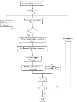
The new SLD is obtained with the computational flow of SLD shown in Figure 1. In step 1, the initial milling force is calculated by initial milling parameters. In step 2, the deflections of workpiece on the nods at first tool position are calculated; then the average deflection of workpiece at first tool position is obtained. In step 3, the actual radial depth of cutting at first tool position is calculated, and the start angle and the exit angle are also calculated. In step 4, the thickness of the first finished workpiece unit is calculated. In step 5, the FRF of workpiece is calculated after the first milling stage. In step 6, the modal parameters of workpiece are extracted from the FRF of workpiece. In step 7, the milling stability is calculated by modal parameters, start angle and exit angle. Then, the stability lobes diagram of first milling stage is obtained. In step 8, repeat the operations from step 1 to step 7 to calculate the milling stability of the next milling stage. After the milling process is completed, the calculation procedure will stop, where𝑚is the number of tool positions.𝑛is the number of nodes on contact locations of tool and workpiece.𝑀is the sum of tool positions and 𝑁 is the sum of nodes on contact locations of tool and workpiece.

3. Time-Varying Model of Deflection and

Dynamic Characteristics of Workpiece

3.1. Calculations of Milling Force and Deflection. The milling process is shown in Figure 2. The workpiece can be simplified into cantilever plate, because the structural stiffness and clamping stiffness of spindle, tool, and fixture are larger enough. Thus, in the finite element models, the bottom of the workpiece is fixed.

Yes

No Initial milling parameters

End Thickness of finished workpiece

Milling force

Workpiece deflection

Actual radial depth of cutting

FRF of workpiece

Milling force Yes

No Milling force

Modal parameters of workpiece

fy(m,n)

dw(m,n)

fy(m,n+1)

n = N

ae(m)

Bm

FRF_w(m)

Start angle_𝜙st(m) Exit angle𝜙ex(m)

m = M SLD_(m)

fy(m+1,n)

Figure 1: Computational flow of SLD.

the workpiece are linearly distributed along the helix direc-tion of cutting edge. Actually, in the milling process of thin-walled components, the radial cutting depth is small and the contact time of cutting edge and workpiece is extremely short because the cutting speed is high. In order to simplify the calculation, the direction is supposed to be straight from the bottom to top at each contact position of tool and workpiece. As shown in Figure 3, the submilling forces load on the central points of every portion of the contact locations.

According to the modeling method of milling force which is presented by Engin and Altintas [15], the angular position of infinitesimal element𝑖on tooth𝑗is defined as follows:

𝜙_𝑗= 𝜙₀+ (𝑗 − 1) 𝜙_𝑝−𝑖𝑑𝑧_𝑅tan𝛽, (1)

where𝜙₀= 2𝜋𝑛_𝑠𝑡/60and𝜙_𝑝= 2𝜋/𝑁_𝑐.

The thickness of milling changes with the variety of the angular positions of cutting edge can be calculated by

ℎ (𝜙𝑗) = 𝑓𝑡sin𝜙𝑗. (2)

Differential tangential and radial cutting forces acting on the infinitesimal of tooth𝑗are given by

𝑑𝐹_𝑡𝑗= 𝑔 (𝜙_𝑗) [𝐾_𝑡ℎ (𝜙_𝑗) + 𝐾_𝑡𝑒] 𝑑𝑧,

𝑑𝐹𝑟𝑗= 𝑔 (𝜙𝑗) [𝐾𝑟ℎ (𝜙𝑗) + 𝐾𝑟𝑒] 𝑑𝑧,

(3)

where

𝑔 (𝜙_𝑗) ={_{ {

1 if 𝜙st< 𝜙𝑗< 𝜙ex

o Tool

Workpiece

Feed dire_ction

z

x

y

Figure 2: Schematic diagram of milling process.

l

l

l

Feed direction Tool position

Act point (node)

2

3

2 3 4

n = 1

1 = m fy

fy

fy

ap

Figure 3: Loading locations of submilling forces.

The start angle and exit angle under up-milling and down-milling can be separately expressed by

𝜙st= 0,

𝜙ex=arccos[1 −

𝑎_𝑒(𝑚) 𝑅 ] ,

(up-milling) ,

Unfinished part (A) Finished part (B)

Nonworking part (C)

Figure 4: Divided parts of workpiece.

𝜙st= 𝜋 −arccos[1 −

𝑎_𝑒(𝑚) 𝑅 ] , 𝜙ex= 𝜋,

(down-milling) . (5)

The deflection of workpiece is induced by milling force, and the actual radial depth of cutting at tool position𝑚can be expressed by

𝑎_𝑒(𝑚)= 𝑎_𝑒−(∑

𝑁

𝑛=1𝑑𝑤(𝑚,𝑛))

𝑁 . (6)

It is noted that 𝑑_𝑤(1,𝑛) are obtained by the initial force calculated with the nominal radial depth of cutting.

The milling force acting on the infinitesimal of tooth𝑗and the submilling force acting on the whole cutting edges, which participate in cutting, are given as follows:

𝑑𝐹_𝑦𝑗= 𝑑𝐹_𝑡𝑗sin𝜙_𝑗− 𝑑𝐹_𝑟𝑗cos𝜙_𝑗,

𝐹_𝑦=∑𝑁𝑐

𝑗=1

𝑀𝑐

∑

𝑖=1

𝑑𝐹_𝑦𝑗. (7)

Thus, the submilling forces acting on the central points of every portion of the contact locations can be obtained by

𝑓_{𝑦(𝑚,𝑛)}= _𝑎𝑙

𝑝 ⋅ 𝐹𝑦. (8)

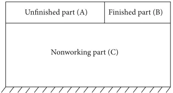
3.2. Calculations of Thickness of Milling Unit. The workpiece element is divided into three parts (Figure 4): unfinished part (A), finished part (B), and nonworking part (C); the thicknesses of A and C are always initial thickness. The part of workpiece which needs milling is divided into𝑚 − 1units by 𝑚tool positions (see Figure 5), and the whole milling process is divided into𝑚 − 1corresponding submilling processes. The units which participate in the milling are composed for B, and other units are for A.

Pm Pm−1 P5 P4 P3 P2 P1

Um−1 · · · U4 U3 U2 U1

Figure 5: Milling units and tool positions.

obvious in a short distance. So, suppose that the deflection on the unit and that on the tool position are approximately equal.

The deflection of workpiece in the submilling process is induced by milling force, and the milling force in the next submilling process is reversely induced by the deflection of workpiece, and so on. The time variation of deflection is represented by the changes of deflections with the changes of submilling processes or tool positions. So, the thicknesses of units are different under the interaction between the milling forces and the deflections.

The thickness of each unit can be obtained by the following equation:

𝐵_𝑚 ={{_{{ {

𝐵₀ 𝑚 = 1

𝐵0− 𝑎𝑒−

(∑𝑁_𝑛=1𝑑𝑤(𝑚,𝑛))

𝑁 𝑚 ̸= 1.

(9)

3.3. Time Variation of Dynamic Characteristics of Workpiece. The dynamic characteristics of workpiece can be represented by time-variant FRF of workpiece which describes the dynamic characteristics in the range of frequency domain. The displacement of workpiece is induced by the milling force acting on the workpiece. The transfer function of workpiece can be expressed by the ratio between the displacement and milling force.

In the material removal, the stiffness characteristics of workpiece material and the loading position are changing. Thus, the FRFs of workpiece are time-variant. Consider

𝐺_𝑦(𝑤)(𝑡) = 𝛿𝑦(𝑤)(𝑡)

𝐹 (𝑡) . (10)

The relationship between the modal mass and the modal damping is satisfied:

𝑚 (𝑡) = 𝑐 (𝑡)

2𝜁 (𝑡) 𝜔𝑛(𝑡), (11)

where𝜁(𝑡) = 𝑐(𝑡)/[2(𝑚(𝑡)𝑘(𝑡))1/2],𝜔_𝑛(𝑡) = [𝑘(𝑡)/𝑚(𝑡)]1/2, and the values of𝑚(𝑡),𝑐(𝑡), and𝑘(𝑡)can be extracted from FRF.

Feed direction

Tool

Workpiece

y

x c(t)

k(t)

Figure 6: Dynamic milling model of workpiece.

4. Milling Stability of Workpiece

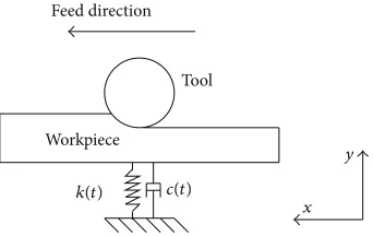
The initial dynamic equation can be established according to the dynamic milling model of workpiece shown in Figure 6. Consider

𝑚 (𝑡) ̈𝑦 (𝑡) + 𝑐 (𝑡) ̇𝑦 (𝑡) + 𝑘 (𝑡) 𝑦 (𝑡) = 𝐹 (𝑡) . (12)

Moreover, the dynamic equation of system can also be expressed as follows [16]:

𝑚 (𝑡) ̈𝑦 (𝑡) + 𝑐 (𝑡) ̇𝑦 (𝑡) + 𝑘 (𝑡) 𝑦 (𝑡)

= −𝑎_𝑝ℎ_𝑦𝑦(𝑡) [𝑦 (𝑡) − 𝑦 (𝑡 − 𝜏)] . (13)

The delayed term𝑦(𝑡 − 𝜏)arises due to the regenerative effect. The time delay is equal to the tooth passing period. The specific cutting force coefficientℎ_𝑦𝑦(𝑡)is determined by the technological parameters:

ℎ_𝑦𝑦(𝑡) =∑𝑁𝑐

𝑗=1

𝑔 (𝜙_𝑗(𝑡))sin𝜙_𝑗(𝑡)

⋅ [−𝐾𝑡sin𝜙𝑗(𝑡) + 𝐾𝑟cos𝜙𝑗(𝑡)] .

(14)

From the viewpoint of dynamical systems, thin-walled workpiece can be defined as the system in which the dynamic characteristics change depending on the tool position, that is, the system considering the effect of machining process on the dynamic characteristics. The thin-walled workpiece milling process is a time-variable parameters system, and the correspondence to the governing equation has the form

̈𝑦 (𝑡) + 2𝜁 (𝑡) 𝜔𝑛(𝑡) ̇𝑦 (𝑡) + 𝜔2𝑛𝑦 (𝑡) =_{𝑚 (𝑡)}𝐹 (𝑡). (15)

Table 1: Geometrical parameters of workpiece.

Category Length (mm) Breadth (mm) Height (mm) Density (g/cm3) Poisson’s ratio Elastic modulus (GPa)

Workpiece 100 3 50 2.7 0.33 69

equations. The convergence of the method was established for a large class of DDEs appearing in engineering applications [18, 19].

The first step of semidiscretization is the construction of the time interval division[𝑡_𝑗, 𝑡_𝑗+1]of lengthΔ𝑡,𝑗 ∈ 𝑁, of the time domain, so that 𝑇 = 𝑘Δ𝑡, where the integer𝑘is called approximation number. By decreasingΔ𝑡, that is, by increasing the approximation number𝑘, the error decreases [18].

Introduce the integer𝑚so that

𝑚 =int( 𝜏

Δ𝑡+ 0.5) , (16)

where𝑚is an approximation parameter regarding the length of the time delay. Details on how to treat this case can be found in [18].

In the𝑗th interval for periodic time𝑇, the periodic DDE (15) can be approximated with the following autonomous ordinary differential equation:

𝑦 (𝑡) + 2𝜁𝜔𝑛,𝑗𝑦 (𝑡) + (𝜔𝑛,𝑗2 + 𝑎𝑝

𝑑_𝑗 𝑚_𝑗) 𝑦 (𝑡)

= 𝑎𝑝

𝑑_𝑗 𝑚_𝑗𝑦𝜏,𝑗,

(17)

where𝑦_𝜏,𝑗= 𝛼𝑦_{𝑗−𝑚+1}+ 𝛽𝑦_𝑗−𝑚≈ 𝑦(𝑡_𝑗+ 0.5Δ𝑡 − 𝜏) = 𝑦(𝑡 − 𝜏), 𝜔𝑛,𝑗= (1/Δ𝑡) ∫_𝑡𝑡𝑗+1_𝑗 𝜔𝑛(𝑡)𝑑𝑡, 𝑑𝑗= (1/Δ𝑡) ∫_𝑡𝑡𝑗+1_𝑗 𝑑(𝑡)𝑑𝑡, and𝑚𝑗=

(1/Δ𝑡)𝑚(𝑡)𝑑𝑡.

By Cauchy transformation, (17) is written in the canonical form

̇

Q(𝑡) =W_𝑗Q(𝑡) + 𝑉_𝑗[𝛼Q_{𝑗−𝑚+1}+ 𝛽Q_𝑗−𝑚] , (18)

where 𝛼 = 𝜏/Δ𝑡 + 0.5 − 𝑚, 𝛽 = 𝑚 + 0.5 − 𝜏/Δ𝑡,W_𝑗 = [−(𝜔2 0 1

𝑛,𝑗+𝑎𝑝(𝑑𝑗/𝑚𝑗) −2𝜁𝜔𝑛,𝑗],Q(𝑡) = {

𝑦(𝑡)

̇𝑦(𝑡)}, V𝑗 = [𝑎𝑝(𝑑𝑗/𝑚𝑗) 00 0], and

Q𝑗 =Q(𝑡𝑗) = {𝑦(𝑡𝑗)̇𝑦(𝑡𝑗)} = { 𝑦𝑗

̇𝑦_𝑗}.

For a given initial conditionQ_𝑗, (18) can be solved in𝑡 ∈ [𝑡_𝑗, 𝑡_𝑗+1]:

Q_𝑗+1=A_𝑗Q_𝑗+B[𝛼Q_{𝑗−𝑚+1}+ 𝛽Q_𝑗−𝑚] , (19)

whereA_𝑗 =exp(W_𝑗Δ𝑡),B_𝑗= (exp(W_𝑗Δ𝑡) −I)A_𝑗−1V_𝑗, and I denotes identity matrix.

According to (19), a discrete map can be defined:

z𝑗+1=P𝑗z𝑗, (20)

where the(𝑚 + 2)-dimensional state vectorz_𝑗is

z_𝑗= [𝑦𝑗 ̇𝑦𝑗 𝑦𝑗−1 ⋅ ⋅ ⋅ 𝑦𝑗−𝑚]𝑇. (21)

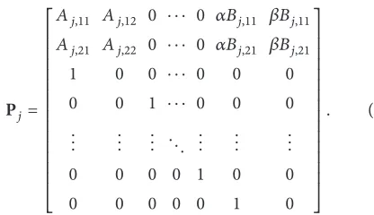
And the coefficient matrixP_𝑗has the form

P_𝑗=

[ [ [ [ [ [ [ [ [ [ [ [ [ [ [ [

𝐴𝑗,11 𝐴𝑗,12 0 ⋅ ⋅ ⋅ 0 𝛼𝐵𝑗,11 𝛽𝐵𝑗,11

𝐴_𝑗,21 𝐴_𝑗,22 0 ⋅ ⋅ ⋅ 0 𝛼𝐵_𝑗,21 𝛽𝐵_𝑗,21

1 0 0 ⋅ ⋅ ⋅ 0 0 0

0 0 1 ⋅ ⋅ ⋅ 0 0 0

... ... ... d ... ... ...

0 0 0 0 1 0 0

0 0 0 0 0 1 0

] ] ] ] ] ] ] ] ] ] ] ] ] ] ] ]

. (22)

Equation (20) makes the connection between states at time𝑡_𝑗and𝑡_𝑗+1. The connection between the states at𝑡₀and 𝑡₀+ 𝑘Δ𝑡 = 𝑡_𝑘is given by coupling of the coefficient matrices in each interval:

Φ =P_𝑘−1P_𝑘−2⋅ ⋅ ⋅P₁P₀. (23)

The stability of (15) can be approximated by the Floquet transition matrix (see (23)). Note that the integer𝑘 deter-mines the number of matrices to be multiplied in (23), and 𝑚determines the size of these matrices.

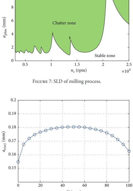
In one milling process, generally, the maximum displace-ment occurs at the top of the workpiece, and the corre-sponding modal shape is first-order bending modal shape of the workpiece. The modal shapes of higher modes are not effective modal shapes. So, using the semidiscretization method [16], the SLD can be obtained by first-order modal parameters as shown in Figure 7. The green zone is chatter domain and the white section is stable domain.

5. Case Study and Experimental Verification

5.1. Numerical Simulation. The geometrical parameters of workpiece are shown in Table 1. The numerical simulations are carried out with the following milling parameters in Table 2.

The simulation results under the axial milling depth of 6 mm are set as an example. As Figure 8 shows, in the milling process, the values of actual radial depth of cutting are different at different tool positions, and the trend of change of that is increased firstly and then decreases. The range abilities of changes are large at the positions of cutting in (𝑋 = 0mm) and cutting out (𝑋 = 100mm). The range abilities of changes are small at the positions closing to the central regions of workpiece (𝑋 = 35–65 mm). The changes of actual radial depth of cutting at tool positions are induced by deflections of workpiece. The value of actual radial depth of cutting at tool position𝑋 = 0mm is the smallest because the workpiece is impacted by the milling force.

Table 2: Parameters of milling process.

Item Value

𝐾_𝑡(N/m2) 5.403×108

𝐾_𝑟(N/m2) 1.81×108

𝐾𝑡𝑒(N/m) 2884

𝐾𝑟𝑒(N/m) 1407

𝑁 3

𝑎𝑝(mm) 4/6/8

𝑎_𝑒(mm) 0.2

𝑅(mm) 3

V(mm/min) 1200

Milling method Down-milling

0.5 1 1.5 2 2.5

0 2 4 6 8 10

Chatter zone

Stable zone

aplim

(mm)

ns(rpm) ×104

Figure 7: SLD of milling process.

0 20 40 60 80 100

0.15 0.16 0.17 0.18 0.19 0.2

X (mm)

ae(m

)

(mm)

Figure 8: Change of actual radial depth at different tool positions.

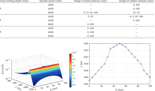
are time-varying; the corresponding values are different at different tool positions as Figure 9 shows. The FRF of workpiece will change corresponding to the changing of the tool positions (see Figure 9(a)) and the first-order natural fre-quency of workpiece has changed in the range from 1045 Hz to 1056 Hz (see Figure 9(b)). The values increased firstly and then decreased with the changes of tool positions. At the same

time, the trend of change of dynamic stiffness at first mode increased firstly and then decreased (see Figure 9(c)). The stiffness of workpiece is large in the center parts and small in the boundary parts. The trends shown in Figure 9 are conformed to the stiffness characteristics of workpiece.

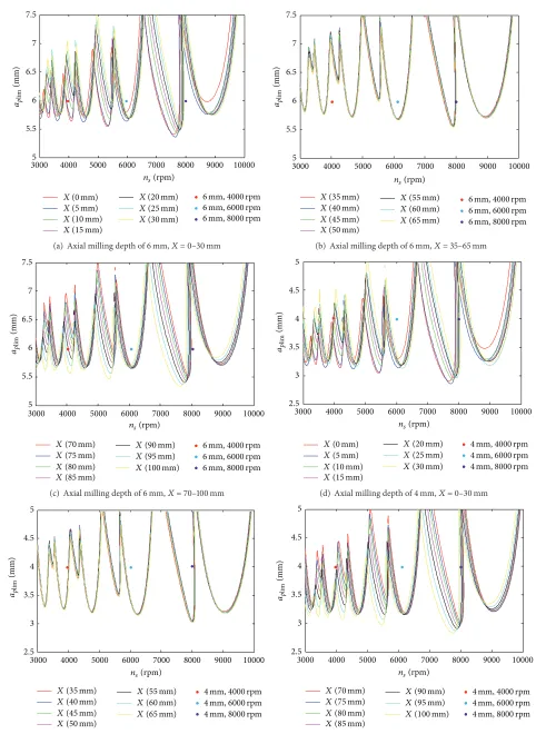
The dynamic milling SLD of workpiece with the axial milling depth of 6 mm are shown in Figures 10(a)–10(c), where the dots with colors in the figures represent the combination of milling parameters. If the red dot is in the stable zone, the milling process is stable under the corresponding combination of milling parameters. If the red dot is in the chatter zone, the milling process is not stable under the corresponding combination of milling parameters. The boundary curves of milling stability move upwards in the right direction with the decrease of deflection and the increases of frequency and minimum dynamic stiffness. Adversely, the boundary curves of milling stability move downwards in the left direction with the increase of deflection and the decreases of frequency and the minimum dynamic stiffness. The stable domain is below the curves and the chatter domain is above the curves. The stable domain and chatter domain are changing with the milling steps in 𝑋-direction under the influences of the time variation of deflection and dynamic characteristics.

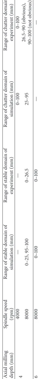
The same laws of change are shown in the dynamic milling SLD of workpiece with the axial milling depth of 4 mm and 8 mm (see Figures 10(d)–10(f) and 10(g)–10(i)). The ranges of stable domain and chatter domain under different combinations of milling parameters are shown in Table 3.

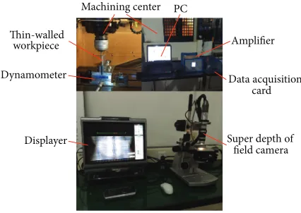
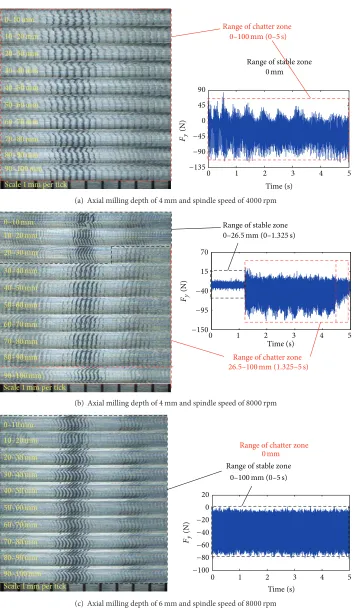
5.2. Experimental Verification. The milling processing is car-ried out by Makino S56 vertical machining center. Kistler 9257B dynamometer is used to measure the milling force and the sampling period of force test is 0.0001 s. The chatter marks on workpiece surface are observed by KEYENCE VHX-1000E super depth of field camera and the photographs are taken with 20x enlargement. The milling experimental equipment is shown in Figure 11. The material of workpiece is aluminum alloy 7075 and that of tool is cemented carbide. Chatter marks on workpiece surface and the test signals of milling force are shown in Figure 12. The length of workpiece is 100 mm, and that of each segment photograph of chatter marks on workpiece surface is 10 mm. It is noted that the deep colors shown in photographs do not represent any meaning and are just caused by reflecting light.

The separation distance between any two adjacent chatter marks on the surface of workpiece is large and the change of amplitudes of milling force is obvious at the axial milling depth of 4 mm and spindle speed of 4000 rpm. The whole milling process is in chatter condition (see Figure 12(a)).

Table 3: Ranges of stable domain and chatter domain under different combinations of milling parameters.

Axial milling depth (mm) Spindle speed (rpm) Range of stable domain (mm) Range of chatter domain (mm)

4

4000 — 0–100

6000 — 0–100

8000 0–25, 95–100 25–95

6

4000 5–95 0–5, 95–100

6000 — 0–100

8000 0–100 —

8

4000 0–100 —

6000 0–100 —

8000 0–100 —

0 20

40 60

80 100 400

600 800

1000 1200

0.5 1 1.5 2 2.5 3 3.5 4 4.5 5

f_(H z) 10−4

10−5

10−6

|G

|

(m/N)

×10−5

20 40

60 80 100 600

800 1000 f_(H

X (mm)

(a) Change of FRF of workpiece at different tool positions

0 20 40 60 80 100

1044 1046 1048 1050 1052 1054 1056

f

(H

z)

X (mm)

(b) Change of first frequency of workpiece at different tool positions

0 20 40 60 80 100

0 1 2 3 4 5

kd

(N/m)

×104

X (mm)

(c) Change of minimum dynamic stiffness of workpiece at different tool positions

Figure 9: Change of dynamic characteristics of workpiece at different tool positions.

two adjacent chatter marks on the surface of workpiece are getting large obviously. In the period of time from 4.5 s to 5 s, the amplitudes of milling force are getting smaller gradually but are larger than those in the first period of time. The separation distance between any two adjacent chatter marks on the surface of workpiece is still large. So, the range of chatter domain is 26.5–100 mm (see Figure 12(b)). The chatter in range of 26.5–90 mm is obvious and that in range of 90– 100 mm is not obvious.

At the axial milling depth of 6 mm and spindle speed of 8000 rpm, the separation distance between any two adjacent chatter marks on the surface of workpiece is homogeneous and the change of amplitudes of milling force is not obvious. The whole milling process is stable (see Figure 12(c)).

30005 4000 5000 6000 7000 8000 9000 10000 5.5

6 6.5 7 7.5

aplim

(mm)

ns(rpm)

X(15mm)

6mm,4000rpm 6mm,6000rpm 6mm,8000rpm

X(0mm)

X(5mm)

X(10mm)

X(20mm) X(30mm) X(25mm)

(a) Axial milling depth of 6 mm,𝑋= 0–30 mm

3000 4000 5000 6000 7000 8000 9000 10000

5 5.5 6 6.5 7 7.5

aplim

(mm)

ns(rpm)

X(35mm) X(₄₀mm) X(45mm) X(50mm)

X(55mm) X(60mm) X(65mm)

6mm,4000rpm 6mm,6000rpm 6mm,8000rpm

(b) Axial milling depth of 6 mm,𝑋= 35–65 mm

3000 4000 5000 6000 7000 8000 9000 10000

5 5.5 6 6.5 7 7.5

ns(rpm)

aplim

(mm)

X(70mm) X(75mm) X(80mm) X(85mm)

X(90mm) X(₉₅mm)

6mm,4000rpm 6mm,6000rpm 6mm,8000rpm

X(100mm)

(c) Axial milling depth of 6 mm,𝑋= 70–100 mm

3000 4000 5000 6000 7000 8000 9000 10000

2.5 3 3.5 4 4.5 5

aplim

(mm)

ns(rpm)

X(10mm) X(15mm)

X(20mm) X(25mm) X(30mm)

4mm,4000rpm 4mm,6000rpm 4mm,8000rpm X(0mm)

X(5mm)

(d) Axial milling depth of 4 mm,𝑋= 0–30 mm

3000 4000 5000 6000 7000 8000 9000 10000

2.5 3 3.5 4 4.5 5

ns(rpm)

aplim

(mm)

X(35mm) X(₄₀mm) X(45mm) X(50mm)

X(55mm) X(60mm) X(65mm)

4mm,4000rpm 4mm,6000rpm 4mm,8000rpm

(e) Axial milling depth of 4 mm,𝑋= 35–65 mm

X(100mm)

3000 4000 5000 6000 7000 8000 9000 10000

2.5 3 3.5 4 4.5 5

ns(rpm)

aplim

(mm)

X(70mm) X(₇₅mm) X(80mm) X(85mm)

X(90mm) X(95mm)

4mm,4000rpm 4mm,6000rpm 4mm,8000rpm

(f) Axial milling depth of 4 mm,𝑋= 70–100 mm

3000 4000 5000 6000 7000 8000 9000 10000 7.5

8 8.5 9 9.5 10

ns(rpm)

aplim

(mm)

X(10mm) X(15mm)

X(20mm) X(25mm) X(30mm)

8mm,4000rpm 8mm,6000rpm 8mm,8000rpm X(0mm)

X(5mm)

(g) Axial milling depth of 8 mm,𝑋= 0–30 mm

3000 4000 5000 6000 7000 8000 9000 10000

7.5 8 8.5 9 9.5 10

ns(rpm)

aplim

(mm)

X(35mm) X(40mm) X(45mm) X(50mm)

X(55mm) X(60mm) X(65mm)

8mm,4000rpm 8mm,6000rpm 8mm,8000rpm

(h) Axial milling depth of 8 mm,𝑋= 35–65 mm

3000 4000 5000 6000 7000 8000 9000 10000

7.5 8 8.5 9 9.5 10

ns(rpm)

aplim

(mm)

X(70mm) X(75mm) X(80mm) X(₈₅mm)

X(90mm) X(95mm)

8mm,4000rpm 8mm,₆₀₀₀rpm 8mm,8000rpm

X(100mm)

(i) Axial milling depth of 8 mm,𝑋= 70–100 mm

Figure 10: Dynamic SLD of milling process with the axial milling depth of 4 mm, 6 mm, and 8 mm.

Machining center PC Thin-walled

workpiece

Displayer Dynamometer

Amplifier

Data acquisition card

Super depth of field camera

0 1 2 3 4 5 Time (s)

Range of chatter zone

Range of stable zone

90

45

0

−45

−90

−135 Fy

(N)

0mm

0–100mm (0–5s)

10–20mm

20–30mm

30–40mm

40–50mm

50–60mm

60–70mm

70–₈₀mm

80–90mm 90–100mm

Scale1mm per tick

0–₁₀mm

(a) Axial milling depth of 4 mm and spindle speed of 4000 rpm

0 1 2 3 4 5

Time (s)

Range of chatter zone

Range of stable zone 10–20mm

20–30mm

30–40mm

40–50mm

50–60mm

60–70mm

70–80mm

80–90mm

90–100mm

Scale1mm per tick

0–10mm

70

15

−40

−95

−150 Fy

(N)

26.5–100mm (1.325–5s) 0–26.5mm (0–1.325s)

(b) Axial milling depth of 4 mm and spindle speed of 8000 rpm

Range of chatter zone

Range of stable zone 10–₂₀mm

20–30mm

30–40mm

40–50mm

50–60mm

60–70mm

70–80mm

80–₉₀mm

90–100mm

Scale1mm per tick

0–10mm

0 1 2 3 4 5

Time (s)

20

0 −20 −40 −60 −80 −100 Fy

(N)

0mm

0–100mm (0–5s)

(c) Axial milling depth of 6 mm and spindle speed of 8000 rpm

6. Conclusions

Chatter has always been a significant problem in thin-walled milling, which is one of the major limitations on productivity and part quality. In order to avoid chatter, the appropriate cutting parameters need to be selected through the stability lobe. In this paper, a new SLD has been presented. The time-varying deflection and dynamic characteristics of workpiece have been considered in the new SLD. This method is based on the identification of the optimal pairs of axial depth of cut and spindle speed at different tool position. The model approaches the actual milling process and has been demonstrated correctly by milling experiment.

Nomenclature

𝜙_𝑗: Angular position of tooth𝑗(∘) 𝜙₀: Initial angular position of tooth𝑗(∘) 𝑛_𝑠: Spindle speed (rpm)

𝑡: Time (s)

𝑗: Number of tool teeth 𝜙_𝑝: Pitch angle (∘)

𝑖: Number of infinitesimal elements on the cutting edge

𝑑𝑧: Height of infinitesimal element on the cutting edge (mm)

𝛽: Helical angle of tool (∘)

𝑅: Radius of tool (mm)

𝑁_𝑐: Sum of tool teeth ℎ(𝜙_𝑗): Cutting thickness (mm) 𝑓_𝑡: Tooth feed rate (mm/tooth)

𝑑𝐹_𝑡𝑗: Differential tangential cutting force acting on tooth𝑗(N)

𝑑𝐹_𝑟𝑗: Differential radial cutting force acting on tooth𝑗(N)

𝑔(𝜙𝑗): Screen function (𝑔(𝜙𝑗) = 1denotes cutting

and𝑔(𝜙_𝑗) = 0denotes no cutting)

𝐾_𝑡: Tangential milling force coefficient (N/m2) 𝐾_𝑟: Radial milling force coefficient (N/m2) 𝐾𝑡𝑒: Tangential linear-edge milling force coefficient

(N/m2)

𝐾_𝑟𝑒: Radial linear-edge milling force coefficient (N/m2)

𝜙_st: Start angle (∘) 𝜙ex: Exit angle (∘)

𝑚: Number of tool positions

𝑛: Number of nodes on contact locations of tool and workpiece

𝑎_𝑒(𝑚): Actual radial depth of cutting at tool position 𝑚(mm)

𝑑_{𝑤(𝑚,𝑛)}: Deflection of workpiece at node𝑛and tool

position𝑚(mm)

𝑑𝐹_𝑦𝑗: Differential milling force in𝑌-direction of tooth𝑗(N)

𝐹_𝑦: Milling force in𝑌-direction (N)

𝑀_𝑐: Sum of differential elements on the cutting edge

𝑓_{𝑦(𝑚,𝑛)}: Submilling force loading on the central points

in every portion of the contact locations (N)

𝑙: Length of every portion (mm) 𝑎𝑝: Axial depth of cutting (mm)

𝑎_𝑒: Nominal radial depth of cutting (mm) 𝑀: Sum of tool positions

𝑁: Sum of nodes on contact locations of tool and workpiece

𝐵₀: Initial thickness of workpiece (mm) 𝐵_𝑚: Thickness of unit (mm)

𝐺_𝑦(𝑤)(𝑡): Transfer function of workpiece with time variation in𝑌-direction (mm/N) 𝛿_𝑦(𝑤)(𝑡): Displacement of workpiece with time

variation in𝑌-direction (mm) 𝐹(𝑡): Dynamic milling force (N) 𝑚(𝑡): Modal mass of workpiece (kg) 𝑐(𝑡): Modal damping of workpiece (N⋅s/m) 𝑘(𝑡): Modal stiffness of workpiece (N/m) 𝜔_𝑛(𝑡): Natural frequency of workpiece (Hz) 𝜁(𝑡): Modal damping ratio of workpiece 𝑦(𝑡): Chatter displacement (mm).

Competing Interests

The authors declare that there are no competing interests regarding the publication of this paper.

Acknowledgments

The authors acknowledge the state S&T projects for upmarket NC machine and fundamental manufacturing equipment of China (no. 2012ZX04012-031, no. 2013ZX04005-013, and no. 2015ZX04005001, resp.).

References

[1] S. Ratchev, S. Liu, W. Huang, and A. A. Becker, “Milling error prediction and compensation in machining of low-rigidity parts,”International Journal of Machine Tools and Manufacture, vol. 44, no. 15, pp. 1629–1641, 2004.

[2] S. Ratchev, S. Liu, W. Huang, and A. A. Becker, “A flexible force model for end milling of low-rigidity parts,”Journal of Materials Processing Technology, vol. 153-154, no. 1–3, pp. 134–138, 2004. [3] E. Budak, “Analytical models for high performance milling. Part

I: cutting forces, structural deflections and tolerance integrity,”

International Journal Machine Tools & Manufacture, vol. 46, pp. 1478–1488, 2006.

[4] J. K. Rai and P. Xirouchakis, “Finite element method based machining simulation environment for analyzing part errors induced during milling of thin-walled components,” Interna-tional Journal of Machine Tools and Manufacture, vol. 48, no. 6, pp. 629–643, 2008.

[5] S. A. Tobias,Machine Tool Vibration, Blackie and Sons, London, UK, 1965.

[6] J. Tlusty and M. Polacek, “The stability of machine Tools against self excited vibrations in machining,” in Proceedings of the ASME Production Engineering Research Conference, pp. 465– 474, 1963.

[8] Y. Altintas,Manufacturing Automation-Metal Cutting Mechan-ics, Machine Tool Vibrations and CNC Design, Chemical Indus-try Press, 2002.

[9] U. Bravo, O. Altuzarra, L. N. L´opez de Lacalle, J. A. S´anchez, and F. J. Campa, “Stability limits of milling considering the flexibility of the workpiece and the machine,”International Journal of Machine Tools and Manufacture, vol. 45, no. 15, pp. 1669–1680, 2005.

[10] S. Herranz, F. J. Campa, L. N. L´opez de Lacalle et al., “The milling of airframe components with low rigidity,”Proceedings of the Institution of Mechanical Engineers, Part B: Journal of Engineering Manufacture, vol. 219, no. 11, pp. 789–801, 2005. [11] T. L. Schmitz, T. J. Burns, J. C. Ziegert, B. Dutterer, and

W. R. Winfough, “Tool length-dependent stability surfaces,”

Machining Science and Technology, vol. 8, no. 3, pp. 377–397, 2004.

[12] A. Tang and Z. Liu, “Three-dimensional stability lobe and maxi-mum material removal rate in end milling of thin-walled plate,”

International Journal of Advanced Manufacturing Technology, vol. 43, no. 1-2, pp. 33–39, 2009.

[13] V. Thevenot, L. Arnaud, G. Dessein, and G. Cazenave-Larroche, “Integration of dynamic behaviour variations in the stability lobes method: 3D lobes construction and application to thin-walled structure milling,” International Journal of Advanced Manufacturing Technology, vol. 27, no. 7-8, pp. 638–644, 2006. [14] Q. Song, X. Ai, and W. Tang, “Prediction of simultaneous

dynamic stability limit of time-variable parameters system in thin-walled workpiece high-speed milling processes,” Interna-tional Journal of Advanced Manufacturing Technology, vol. 55, no. 9-12, pp. 883–889, 2011.

[15] S. Engin and Y. Altintas, “Mechanics and dynamics of general milling cutters. Part I: helical end mills,”International Journal of Machine Tools & Manufacture, vol. 41, no. 15, pp. 2195–2212, 2001.

[16] T. Insperger and G. St´ep´an, “Updated semi-discretization method for periodic delay-differential equations with discrete delay,”International Journal for Numerical Methods in Engineer-ing, vol. 61, no. 1, pp. 117–141, 2004.

[17] T. Insperger, B. P. Mann, G. St´ep´an, and P. V. Bayly, “Stability of up-milling and down-milling. Part 1. Alternative analytical methods,”International Journal of Machine Tools & Manufac-ture, vol. 43, no. 1, pp. 25–34, 2003.

[18] T. Insperger and G. St´ep´an, “Semi-discretization method for delayed systems,”International Journal for Numerical Methods in Engineering, vol. 55, no. 5, pp. 503–518, 2002.

[19] F. Hartung, T. Insperger, G. St´ep´an, and J. Turi, “Approximate stability charts for milling processes using semi-discretization,”

International Journal of

Aerospace

Engineering

Hindawi Publishing Corporation

http://www.hindawi.com Volume 2014

Robotics

http://www.hindawi.com Volume 2014

Hindawi Publishing Corporation

http://www.hindawi.com Volume 2014

Active and Passive Electronic Components

Control Science and Engineering Journal of

Hindawi Publishing Corporation

http://www.hindawi.com Volume 2014

Machinery

Hindawi Publishing Corporation

http://www.hindawi.com Volume 2014

Hindawi Publishing Corporation http://www.hindawi.com

Journal of

Engineering

Volume 2014

Submit your manuscripts at

http://www.hindawi.com

VLSI Design

Hindawi Publishing Corporation

http://www.hindawi.com Volume 2014

Hindawi Publishing Corporation

http://www.hindawi.com Volume 2014 Shock and Vibration

Hindawi Publishing Corporation

http://www.hindawi.com Volume 2014

Civil Engineering

Acoustics and VibrationAdvances in Hindawi Publishing Corporation

http://www.hindawi.com Volume 2014 Hindawi Publishing Corporation

http://www.hindawi.com Volume 2014 Electrical and Computer Engineering

Journal of

Advances in OptoElectronics

Hindawi Publishing Corporation

http://www.hindawi.com Volume 2014

The Scientific

World Journal

Hindawi Publishing Corporation

http://www.hindawi.com Volume 2014

Sensors

Hindawi Publishing Corporation

http://www.hindawi.com Volume 2014

Modelling & Simulation in Engineering

Hindawi Publishing Corporation

http://www.hindawi.com Volume 2014

Hindawi Publishing Corporation

http://www.hindawi.com Volume 2014

Chemical Engineering

International Journal of Antennas and

Propagation International Journal of

Hindawi Publishing Corporation

http://www.hindawi.com Volume 2014

Hindawi Publishing Corporation

http://www.hindawi.com Volume 2014

Navigation and Observation International Journal of

Hindawi Publishing Corporation

http://www.hindawi.com Volume 2014

Distributed

Sensor Networks