Robust arbitrary view gait recognition based on 3D partial similarity matching

warwick.ac.uk/lib-publications

Original citation:

Tang, Jin, Luo, Jian, Tjahjadi, Tardi and Guo, Fan. (2016) Robust arbitrary-view gait

recognition based on 3D partial similarity matching. IEEE Transactions on Image Processing .

doi:

10.1109/TIP.2016.2612823

Permanent WRAP URL:

http://wrap.warwick.ac.uk/82258

Copyright and reuse:

The Warwick Research Archive Portal (WRAP) makes this work by researchers of the

University of Warwick available open access under the following conditions. Copyright ©

and all moral rights to the version of the paper presented here belong to the individual

author(s) and/or other copyright owners. To the extent reasonable and practicable the

material made available in WRAP has been checked for eligibility before being made

available.

Copies of full items can be used for personal research or study, educational, or not-for profit

purposes without prior permission or charge. Provided that the authors, title and full

bibliographic details are credited, a hyperlink and/or URL is given for the original metadata

page and the content is not changed in any way.

Publisher’s statement:

© 2016 IEEE. Personal use of this material is permitted. Permission from IEEE must be

obtained for all other uses, in any current or future media, including reprinting

/republishing this material for advertising or promotional purposes, creating new collective

works, for resale or redistribution to servers or lists, or reuse of any copyrighted component

of this work in other works.

A note on versions:

The version presented here may differ from the published version or, version of record, if

you wish to cite this item you are advised to consult the publisher’s version. Please see the

‘permanent WRAP url’ above for details on accessing the published version and note that

access may require a subscription.

Abstract—Existing view-invariant gait recognition methods encounter difficulties due to limited number of available gait views and varying conditions during training. This paper proposes gait partial similarity matching that assumes a 3-dimensional (3D) object shares common view surfaces in significantly different views. Detecting such surfaces aids the extraction of gait features from multiple views. 3D parametric body models are morphed by pose and shape deformation from a template model using 2-dimensional (2D) gait silhouette as observation. The gait pose is estimated by a level set energy cost function from silhouettes including incomplete ones. Body shape deformation is achieved via Laplacian deformation energy function associated with inpainting gait silhouettes. Partial gait silhouettes in different views are extracted by gait partial region of interest elements selection and re-projected onto 2D space to construct partial gait energy images. A synthetic database with destination views and multi-linear subspace classifier fused with majority voting are used to achieve arbitrary view gait recognition that is robust to varying conditions. Experimental results on CMU, CASIA B, TUM-IITKGP, AVAMVG and KY4D and datasets shows the efficacy of the propose method.

Index Terms—gait; person identification; 3D gait model; partial similarity matching.

I. INTRODUCTION

AIT is difficult to be disguised and can be easily

observed in low-resolution video sequences at long distance without contact with the human subject. Thus gait recognition has great potential, and could be useful in various scenarios, such as analysis of forensic evidence for a legal case [1], criminal investigation and security check [2]. It could be achieved with high recognition rate where environmental and certain factors are controlled to some extent. The gait database OU-ISIR LP with 4000 subjects [3] has been used to evaluate the upper bound accuracy of gait recognition. However, implementing a gait-based personal identification system for large population in a real application is still

This work was supported partly by the National Natural Science Foundation of China (Grant No.61403426, No.91220301), the Scientific Research Project of Hunan Provincial Education Department, China (Grant No.15C0981), and the Science and Technology Key Program of Hunan, China (Grant No.2015WK3006).

J. Tang is with the School of Information Science and Engineering, Central South University, Changsha, Hunan 410083, China ([email protected]).

J. Luo is with the School of Information Science and Engineering, Central South University, Changsha, Hunan 410083, China ([email protected]).

T. Tjahjadi is with the School of Engineering, University of Warwick, Gibbet Hill Road, Coventry, CV4 7AL, United Kingdom, ([email protected]).

F.Guo is with the School of Information Science and Engineering, Central South University, Changsha, Hunan 410083, China ([email protected])

challenging due to the imaging of natural gait being easily influenced by various factors, such as scene structure, illumination, clothing variation, footwear, carrying conditions, walking speed, occlusions and camera views [4-6]. Nevertheless, gait provides an additional biometric cue for reliable personal identification system.

In order to obtain acceptable recognition rate, it is important to obtain good segmentation of the gait silhouettes. However, many factors often lead to inaccuracy in the segmentation, e.g., similarity of colours between the subject’s clothes and background, changes in background due to illumination or appearance of new objects, self occlusion, etc. [7]. Gait image inpainting methods have thus been proposed, i.e., partial derivative equations based, texture synthesis, semi-automatic inpainting and hybrid methods. Multiple filters have been introduced to reduce noise or enhance the image quality. Image matching and moving object detection have been used to address dark areas of the data and to perform hole-filling. However, these methods assume that the missing pixels are similar to their adjacent pixels and thus use neighbouring pixels for interpolation. When the missing data is large, e.g., due to significant occlusion, existing model-free inpainting methods fail to correctly segment the gait silhouettes. Other methods for addressing imperfect gait silhouettes use robust statistics to extract gait features in a static image by averaging the silhouettes in a gait period. The gait energy image (GEI) [8] is one such method that is less sensitive to uncorrelated silhouette noise. Other variants include Gait Flow Image (GFI) [9], Pose Kinematics and Pose Energy Image (PEI) [10] and Frame Difference Energy Image (FDEI) [7]. However, these energy images are mainly for mitigating the effect of imperfect silhouettes in covariate conditions that affect gait feature extraction rather than the gait itself. Thus, in this paper we introduce a gait inpainting method that uses the unified and prior knowledge of 3D human body to restore the incomplete gait silhouettes when there is large missing data.

Existing 2-dimensional (2D) gait recognition systems encounter difficulties in multi-view gait recognition where there is a limited number or absence of some gait views in the training data. Since gait is 3-dimensional (3D), a 2D gait image sequence provides only single-view information that constrains gait recognition from an arbitrary view. Using 2.5 dimensional (2.5D) or 3D models for gait recognition [11,12] has achieved significant advances due to the availability of 3D imaging devices where the data is used for 3D reconstruction and target tracking. However the use of inexpensive 3D

Robust Arbitrary-View Gait Recognition based

on 3D Partial Similarity Matching

Jin Tang, JianLuo

*

_{,Tardi Tjahjadi, and Fan Guo}

sensors has its limitations, e.g., low-resolution and unreliable coarse range data for dark and infrared-absorbing objects, missing data if the objects are out of the sensor’s range, and data flickering in successive frames. Thus, it is difficult to use only range data to accurately segment body contours. The coarse data of the head and feet are also sometimes missing. As a result the 2.5D gait voxel models derived from the coarse range images are also imperfect. The use of such an approach provides only partial view of the gait data, similar to the use of a 2D camera. It only provides a simplified 3D surface

representation that contains one range value (z) for every point

in the (x, y) image plane. The use of high-accuracy 3D whole

body scanners are typically expensive and limited for static modelling due to the long scanning time, e.g., for estimation of the body shape beneath the clothes.

For view-invariant gait recognition to be practical, few cameras should be used. In this paper, we use 2D gait images that include incomplete body images to estimate the 3D gait model. The 3D gait pose is first estimated using level set energy cost function and improved using Laplacian deformation. The method not only repairs the incomplete 2D gait images but also estimates its corresponding 3D model. Since only one-view gait images are used, the 3D model is imperfect. Thus, a gait partial similarity matching (GPSM) is proposed for extracting the partially matched gait features in a cycle from 3D gait models with different views. These are the common data of a surface viewed from significantly different camera locations, referred to as the common view surface. Detecting the common view surfaces in different views and transforming the surfaces to the same view aids the extraction of the gait features from multiple views. We refer this as gait partial similarity matching and use it to achieve gait recognition from different views, especially for probe data from view that is not in the training dataset, i.e., gait recognition from arbitrary views but with limited number of gait views available during training.

The contributions of this paper are: (1) use of 3D human pose estimation and shape deformation to reconstruct parametric 3D body from 2D data to achieve robustness to variation in significant view changes, and occlusions, e.g., missing body parts or segmentation noise; (2) use of 2D incomplete gait image inpainting with weighted level set function based on 3D body to significantly improve the quality of incomplete 2D gait silhouettes for improved recognition; (3) by using partial similarity matching, view-invariant 2D gait images can be matched directly by partial similar features enabling robustness to carried item and improved recognition rate; and (4) by introducing multi-linear subspace classifier with majority voting for fusion enables arbitrary views gait recognition using GPSM.

This paper is organized as follows. SectionⅡpresents the

related work. Section Ⅲ discusses the gait partial similarity

matching. Section Ⅳ presents our multi-view gait recognition

method based on multi-linear subspace classifier with majority

voting. SectionⅤpresents the experimental results and Section

Ⅵ concludes the paper.

II. RELATED WORK

There are two main approaches to view-invariant gait recognition: (1) model-based human body structural analysis and (2) model-free appearance-based statistical analysis. The first approach uses different 3D gait skeleton structural models for view-invariant feature extraction of length of torso, upper arm, lower arm, thigh, calf and foot [13]. Zhao et al. [14] explored the use of multiple cameras to construct skeleton model with 10 joints and 24 degree of freedom. The length of key segments are extracted as static parameters, and their motion trajectories used as dynamic features to realize 3D gait recognition. Rogez et al. [15] modelled 3-D body poses and camera viewpoints with a low dimensional manifold, and use it to learn a generative model of the silhouette for view invariant 3-D gait tracking. However all current modelling of 3D gait skeleton structural models is mostly based on images from multiple cameras, and are thus inaccurate. Also the features extracted from these models are limited.

The second approach uses 3D appearance, 2D image appearance or 2.5D depth image appearance. Shakhnarovich et al. [16] used an image-based visual hull to construct a 3D model that is rotated to realize view-invariant gait recognition by projecting 3D surface to 2D space. Sivapalan et al. [17] used a 3D volume model derived from multi-view 2D images or frontal depth images, and the back-filled versions for matching frontal-view depth image and side-view 2D silhouette for cross-modal cross-view gait recognition. However, the need of complex hardware setup makes it practical only under limiting laboratory setting.

There are three approaches to 2D appearance-based gait recognition. The first adopts view normalization or uses the result fused from multiple view-dependent gait recognition. Nizami et al. [18] used Extreme Learning Machine multiclass classifier where the view-dependent classifications are fused at score level according to some rules. This method is limited by the size of the multi-view gait databases and cannot realize arbitrary-view gait recognition. Jean et al. [19] used view-normalized body part trajectories as view-invariant gait features, but these are impractical for significantly different views and when self-occlusion is encountered. Wei et al. [20] introduced the deterministic learning theory to achieve view-invariant gait recognition and extraction of gait silhouette features that represents gait dynamics and reflects view variation.

The second uses projection relationship of gaits across different views. Makihara et al. [21] proposed a view transformation model (VTM) to transform a probe gait view data onto the virtue view that exists in the training database. Muramatsu et al. [22] proposed arbitrary gait view transformation scheme using 3D gait data via VTM. Kusakunniran et al. [23,24] developed a VTM by using correlated motion regression and multi-layer perceptron. However a VTM based method requires multi-view 2D images to construct the VTM and performs virtue view transformation during recognition. Also, the parameters of the VTM are sensitive to the training multi-view images.

view-invariant discriminative projection to improve the discriminative ability of multi-view gait features using a unitary linear projection. The multi-view gait features are matched without knowing or estimating the viewing angles. Hu et al. [26] used a sparse local discriminant canonical correlation analysis (CCA) to model the correlation of gait features from different views, using the correlation strength as similarity measure. Multi-view gait features correlation analysis does not require the gait to be transformed to virtue view. However, the gait features are less correlated when the gait views are significantly changed, and multi-view gait images are needed in the training step.

Numerous gait recognition methods have been proposed to address multiple covariates (e.g., occlusion, clothing invariant, carrying items, and unconstrained paths). Martín-Félez et al. [27] treat gait recognition as a bipartite ranking problem. By exploiting learning to rank, the method is suitable under an uncooperative setting and robust against changes in covariate conditions. To identify subjects walking along curved trajectories Iwashita et al. [28] used a 4D gait database to synthesize virtual image corresponding to the estimated direction, and affine moment invariants as gait features. Rida et al. [29] select the most discriminative body part based on group Lasso of motion to reduce the intra-class variation. Xin et al. [30] used integrated sparse coding and multi-view hypergraph learning for recognizing a pedestrian under uncooperative setting. López-Fernández et al. [31] presented a rotation invariant gait descriptor based on 3D angular analysis of the subject’s movement for multi-view gait recognition on unconstrained paths. Nandy et al. [32] used pooled segmented statistical features to describe the shape of GEI edge contour. The higher order moments of the shape centroid in conjunction with a set of other area based features are combined to improve the classification results. Most of these methods address different covariates with limited gait views, mainly using frontal or side view of the gait sequences. In fact, it is difficult for a 2D training dataset to cover all conditions, especially incomplete gait silhouettes and with different carrying that affect the overall body shape directly.

To address the above-mentioned gait recognition problems with arbitrary views, we propose partial similarity matching based on reconstructed 3D gait model with inpainting. A single view gait image is used to estimate the 3D gait model that includes one-side virtual surface portion of the human body in a gait cycle. The partial gait silhouettes in different views are extracted using gait partial region of interest (ROI) elements selection method and re-projected onto 2D space to construct partial gait energy images (PGEIs). A synthetic database with destination views is constructed based on GPSM, and multi-linear subspace classifier fused with major voting is used for gait classification and subject identification.

III. GAIT PARTIAL SIMILARITY MATCHING A. Overview

GPSM in 3D space enables gait recognition from different views especially from arbitrary views using limited number of gait views available in training data as illustrated in Fig.1. In

Euclidean space, given two different 3D surface modelsS₁and

2

S , the 3D partial surface matching searches for the optimal

transformation

T

=

{ , }

R t

, where R is rotation matrix and t is

translation matrix, by solving

2 ( , )

arg min

_{v v C}

T

Rv t v

ʹ′ ∈

+

−

ʹ′

∑

(1)

where C denotes the dataset of GPSM points between the two

surfaces. Most methods for solving 3D partial similarity matching, e.g., Besl [33] and Bareque [34], use two static 3D images of the same object captured at different views, and a

rigid transformation T. As a gait cycle is composed of several

dynamic non-rigid body transformation models, it is difficult

to just use T to match the training subjects with themselves or

with each other. Thus, in this paper a partial similarity matching (based on selected gait partial ROI elements between the given views) and PGEIs as features are used to realize arbitrary view gait recognition.

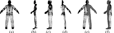
[image:4.612.332.552.259.323.2]

(a) (b) (c) (d) (e) (f) Fig. 1. Gait partial similarity matching: (a) mesh vertices at 0° view (i.e., front view); (b) 90° view partial mesh vertices obtained by removing the self-occlusion data in (a) and rotated to 90°; (c) mesh vertices at 90° view; (d) 0° view partial mesh vertices obtained by removing the self-occlusion data in (c) and rotated to 0°; (e) grey part of body denotes the partial similarity matching of (a) and (c) at 0° view using (d) as partial feature; and (f) grey part of body denotes the partial similarity matching of (a) and (c) at 90° view using (b) as partial feature.

[image:4.612.317.563.593.723.2]

The overview of the partial similarity matching is shown in Fig. 2. In order to reconstruct the 3D gait model with different poses, a low DoF articulated skeleton structure is embedded into the body mesh, and a level set energy cost function is used for estimating the gait pose from incomplete 2D gait silhouettes. Laplacian deformation is then performed and the estimated pose mesh fitted onto the detailed body shape using the repaired 2D gait silhouette contour as reference. The gait frames used for 3D reconstruction are captured by a single view camera and include only the front view of the human body as silhouette constraints. Due to the absence of the side or rear surfaces, GPSM is used for partial similar feature extraction and representation. The multi-view PGEIs are then obtained to form a novel synthetic gallery database for multi-view gait training. Multi-linear subspace analysis with majority voting is used for subject identification.

Gallery sequences

Gallery sequences

Probe sequences

Probe sequences

GPSM Feature Extraction

Gait Partial ROI Elements Selection

Gallery Partial Gait Energy Image

GPSM Feature Extraction

Gait Partial ROI Elements Selection

Probe Partial Gait Energy Image

Synthetic Multi-view

DB with destination

views

Multi-linear Subspace Analysis

Majority voting

Identification Pose Estimation

3D Reconstruction

3D Reconstruction

Template based Gait inpainting

Shape Deformation Parametric 3D

Gait Model

B. 3D gait model reconstruction

In 2D space, due to the absence of range value for every point in the image plane, partial similarity matching features cannot be extracted directly. Also, most research on 3D human motion capture assumes the body shape is known and is represented coarsely (e.g., using cylinders or super quadrics to fit limbs, or using visual hull without skeleton embedded). Such representations are less useful for 3D gait recognition with covariates. To address these problems, a parametric 3D human body is chosen as a template model obtained using the software Makehuman [35] that incorporates 1170 morphings. The parametric body model is optimized for subdivision surfaces modelling with 15128 vertices, suitable for gait modelling. Since gait silhouettes are often imperfect, by using parametric template, the model based gait silhouette inpainting can be derived for 3D gait model reconstruction.

The reconstruction of 3D gait model from incomplete 2D gait silhouettes involves the following steps: 1) initialize the 3D parametric body template; 2) estimate 3D body pose; 3) template based 2D incomplete gait image inpainting; and 4) 3D shape deformation using the complete 2D gait silhouette.

1) Initializing 3D parametric body template

A standard T-pose 3D parametric body is derived from the Makehuman software with average semantic values as shown in Fig. 1(a). Since T-pose body is not well fitted with the human postures in a gait cycle, a model with an I-pose as shown in Fig. 1(b) is initialized as 3D body template by morphing T-pose model onto I-pose using skeleton-based mesh deformation method [36]. The template model mesh is

parameterized by the vector X=

_{

V TX, X

_}

comprising M

vertices V_X =

_{

v v₁, ,..., ,...,₂ v_m v_M

_}

and I mesh faces

{

1, , ,2 I

}

T= t t L t . We use an articulated skeleton structure

from [37] as shown in Fig. 3(c).

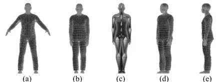
(a) (b) (c) (d) (e)

Fig. 3. 3D body template mesh: (a) T-pose 3D parametric body mesh; (b) initialized I-pose body mesh at 0°view; (c) skeleton embedded in I-pose model mesh; (d) I-pose model at 45° view; and (e) I-pose model at 90° view.

It is assumed that the surface of template X comprises the

set of P=

_{

p p₁, ₂,...,pj,...,pJ

_}

rigid parts that are associated

with J joints of the articulated skeleton. Every vertex in the

template model is associated with a part label

η

_j. It denotes

the rigid part to which the vertex belongs. Every rigid part p

is associated with a set of vertices and it has the same set of transformations in pose deformation, i.e., the joint rotation. The rigid parts of the human body are associated with the body joints and are estimated using the algorithm in [38].

2) Estimation of 3D body pose based on energy cost function

Most recent work on body pose estimation and tracking using image cost function or other Bayesian methods require a

generative model. However, crude and structured models are often used, e.g., articulated body model or ellipsoidal parametric model [39]. The method for recovering 3D pose throughout an image sequence by using SCAPE parametric body models in [40] based on 2D images assumes that the level of detailed shape recovery can be improved with additional cameras and improved background subtraction.

Let

S x y

( , )

be the RGB frame captured by a fixed camera.

Binary human silhouette image

S x y

( , )

is extracted using the

background subtraction algorithm in [41] which can cope with local illumination changes, such as shadows and highlights, as well as global illumination changes. However, gait silhouettes extracted from a complex environment might still be incomplete, e.g., those in Fig. 4, where large areas of the silhouette are missing, mainly due to the similarity of colours between the subject’s clothes and background. It is thus important to estimate the detailed 3D body shape and pose directly from the incomplete images.

[image:5.612.340.538.270.347.2]

(a) (b) (c) (d)

Fig. 4. 2D incomplete gait silhouettes from CASIA databse.

In this paper, the observation 2D gait silhouette images (complete or incomplete) are used to estimate 3D body poses.

Let the estimated 3D gait model be denoted by Y=

_{

V T_Y, _Y

_}

andV_Y =

_{

y y₁, ,... ,...,₂ y_n y_M

_}

where M is the number of

vertices. The instance model Y is obtained from the template

model X with pose deformation. The body pose is associated

with the joint angles of model skeleton. The vertices of the

new pose deformed model Yis denoted by

{

( ( ))

}

Y m m

V = v R⋅ Δ

α

_ξ , (2)

whereΔα is joint relative rotation angles,m=1K M, vmare

vertices in V_X of template model,Ris rigid part transform

matrix,

ξ

( )

m

∈

η

j

,

j

=

1,2,...,

J

determines to which rigid part

m

v belongs,

η

_j is part label, and

1 2

[ _{η η} ... _ηJ]

ψ

= Δ

α

Δ

α

Δ

α

which is denoted by the joints rotation matrix from the template I-pose model. Using the joint relative rotation angles, a hierarchical skeleton with rigid bones connected by joints is constructed. The 3D mesh model is skinned to the given posture using the method in [36], i.e., the template 3D I-model is morphed onto any given posture.

Level set was introduced in [42] for capturing moving fronts to address image segmentation problems. We do not use the level set directly for gait contour segmentation from complicated background images. Instead, we apply level set algorithm to incomplete 2D gait silhouettes to construct pose

energy cost function,E_t, image inpainting and gait image

inpainting with 3D templates for estimation of body pose. Let the moving active contours or moving front be denoted

[image:5.612.59.283.463.545.2]

( , , )

t x y

φ

is the level set function at time t. The evolution

equation of level set function is

0

F t

φ

φ

∂

+ ∇ =

∂ , (3)

where F denotes the speed function. In image segmentation F

is associated with the level set function

φ

and the gradient of

the image data. The level set function at time t is usually

defined as a signed distance function

( , ( ))

( ( , ), ) 0 ( )

( , ( ))

d r t r

r x y t r t

d r t r

ζ

φ

ζ

ζ

+

−

⎧ ∈ Ω

⎪

=_⎨ ∈

⎪_{− ∈ Ω}

⎩

v v

v v

v v (4)

where

r x y

v

( , )

is the spatial vector determined by the point

( , )

x y

in 2D image plane, and

d r

( , ( ))

v

ζ

t

denotes the signed

distance between vector rv and the zero level set active

contour

ζ

( )

t

at time t. The distance function

d r

( , ( ))

v

ζ

t

is

defined as

d r

( , ( )) min(

v

ζ

t

=

r r

v v

−

_I

)

, where

r

I

∈

ζ

( )

t

v

_. +

Ω

denotes the area outside the active contour while −

Ω

is inside.

The level set function is re-initialized periodically to be a signed distance function during evolution by solving

0

( )(1 ) sign

t

φ

φ

φ

∂

= − ∇

∂ . (5)

Since the re-initialization is quite complex, we use the variational level set formulation of curve evolution without re-initialization [43], i.e.,

( ) ( ) ( ) ( )

div div g vg

t

φ

φ

φ

µ

φ

λδ φ

δ φ

φ

φ

⎡ ⎤

∂ ∇ ∇

= _⎢Δ − + + _⎥

∂ ⎢_⎣ ∇ ∇ ⎥_⎦

(6)

where λ> 0,µ and ν are constants. The edge indicator

function

2

1 1 g

G_σ I

=

+∇ ∗

, (7)

where G is the Gaussian kernel with standard deviation σ.

The approximation of (6) is expressed as [43]

1

, , ( , )

k k k

i j i j L i j

φ

+

φ

τ φ

= + , (8)

where ( k_, )

i j

L

φ

is an approximation of the right hand side of (6)

by the partial difference scheme (4).

The performance of level set depends on how its parameters are set, especially for complex background. We use the level set method to process incomplete gait silhouettes, e.g., Fig. 5(a), and construct level set images, e.g., Fig. 5(e)-(f). For our

gait silhouettes, we used the parameters λ=5.0, µ=0.04, ν=3.0,

and time stepτ=5.0 as similarly used in [43], which is

significantly larger than the time step used for traditional level

set methods. The curve evolution takes 300 iterations.

Let the observation 2D gait image shown in Fig. 5(a) be

denoted by

I

₂D

( , )

x y

and the corresponding 3D to 2D

mapping gait image beI x y_Yθ_t( , )_{as illustrated in Fig. 5(d),}

which is derived from the estimated 3D gait model Y_{t at time}

t. Y_{t as illustrated in Fig. 5(c) is morphed from template}

I-pose gait mesh model using human skeleton skinned mesh animation method. The level set method is used to obtain the

silhouettes of the two gait images, where the final evolution

level sets are denoted by

_φ

_2D and

_φ

_3D . The silhouette

contours are denoted by 0

2d 2D

( , ) 0

x y

ζ

=

φ

=

and

0

3d 3D

( , ) 0

x y

ζ

=

φ

=

. The data inside the silhouette contours

have negative value φ<0while the data outside the contours

have positive value φ>0 as illustrated in Fig.5.

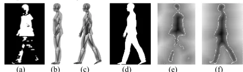
(a) (b) (c) (d) (e) (f)

Fig. 5. Level set of gait images: (a) 2D incomplete gait image; (b) I-pose 3D body template mesh with skeleton embedded; (c) estimated 3D gait model by posture morphing from (b); (d) 2D projected gait image from morphed mesh (c); (e) level set of (a) in X-Y plane; and (f) level set of (d) in X-Y plane.

Let the level set of the observation 2D gait image

1

2D 2D

H

(

2D

)

H

(

2D

)

φ

=

φ

−

φ

+

φ

be 1 where

φ

_2D

>

0

and retain the

value unchanged for

φ ≤

₂D

0

as shown in Fig. 6(a), where

( )

H

⋅

is the Heaviside function. The gait data inside the level

set contour of 3D projected gait image is extracted and

denoted by

S

₃D

=

H

(

−

φ

₃D

)

. The data set inside the level set

contour are then weighted by

0 3

( , )

( ,

)

w d

D x y

=

G

_σ

∗

d r

v

ζ

, (9)

where 0

3

( ,

d

)

d r

v

ζ

denotes the distance between vector

r x y

v

( , )

and curve 0

3d

ζ

.

G

_σ is the Gaussian kernel with standard

deviation σ. * denotes the convolution operation and (⋅)

denotes the dot product between two matrices. Let

1

2

(

3

)

mix D

D S

w D

φ

=

φ

⋅

⋅

which is the weighted mixture of the

two level set shown in Fig. 6(c).

[image:6.612.318.563.137.210.2]

(a) (b) (c) (d) (e)

Fig. 6. Level set energy cost function construction: (a) processed level set of 2D incomplete gait image; (b) 3D projected gait silhouette after weighting; (c) mixture of the two data sets of (a) and weighted silhouette (b); and (d) and (e) are mixture of the data set of (a) and two different pose projected silhouettes without weighting.

The mixed level set

_φ

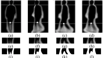
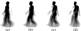
_mix is then segmented into three parts,

the human silhouettes are sometimes incomplete. To overcome this, the frames of gait silhouettes in a cycle are first averaged using GEnI [46] as illustrated in Fig 7(a)-(d) without the horizontal lines. The lower part of GEnI between anatomical positions hip and knee are segmented as shown in Fig. 7(e)-(h) and converted to binary images, i.e., Fig. 7(i)-(l). Using the corresponding binary images, the fixed point of pendulum is estimated from the position of the second peak.

(a) (b) (c) (d)

(e) (f) (g) (h)

[image:7.612.75.275.142.253.2]

(i) (j) (k) (l)

Fig. 7. Segmentation of sub-level set parts using GEnIs: (a)-(d) GEnIs in 18°, 54°, 90°, 126° views withhorizontal lines as estimated positions of shoulder and pendulum; (e)-(h) segmented parts between hip and knee from (a)-(d); and (i)-(l) corresponding binary images of (e)-(h).

Let

H

s

=

0.870

H

be the anatomical position of neck. The

estimated position, which might be closer to the actual

location, is defined as

H

ˆ

s

∈

[

H

s

−

△

h H

s

+

△

h

]

, where

△

h

denotes the interval parameter. Let _ˆ

s H

L

denotes the slice width

from left to right body contour in

H

ˆ

_s horizontal position. The

value of

H

ˆ

_{s is estimated by} ˆ

ˆ [ ]

ˆ

_{arg min}

s

s s s

s H

H H h H h

H

L

∈ − +

=

△ △

.

Let the sub level set body parts be denoted by n

mix

φ

where

n=1, 2, 3. The level set energy cost function is

3

1

i i

t neg neg mix mix i

E

µ

E

µ

E =

=−

_∑

+ , (10)

where

1

( )

i i i

neg mix _{mix L}

E = H −

φ

⋅

φ

and _mix ( _mix( , ))

x y

E =

_∑∑

φ

x y .

0

i neg

µ

> and

µ

mix

>

0

are the weighted coefficients. The 3D

body pose estimation aims to obtain the optimal joints rotation matrix from template I model which is determined by

1 2

[ _{η η} ... _ηJ]

ψ

= Δ

α

Δ

α

Δ

α

. This is achieved by calculating the

minimal energy cost

1 2

[ ... ]

arg min

J

t

E

η η η

ψ α α α

ψ

=Δ Δ Δ

ʹ′= . (11)

Fig. 6 illustrates the construction of the energy cost

function which includes two parts. One is denoted by i

neg E

which indicates how close the two silhouettes agree with each other in global space. If the silhouettes fit each other well, this indicates the largest level set overlap region. The level set data inside the gait contour regions has negative value and we use

i neg E

− to indicate the sum. We also segment the mixed level

set into three parts in order to overcome the sub-optimal decisions when significant part of the body is lost. The legs usually have the higher weighted coefficient because they are associated with the most important body motion for gait recognition. If there is a significant loss in data the leg regions would have small energy compared with other body parts and

thus have make little effect or can even be ignored in the cost function. In order to address the solution being trapped in local optimum, the higher weighted coefficient is used. The other

part of the cost function is denoted by

E

_mix which aids in

improving the accuracy of the incomplete silhouette fitting process. Fig. 6(d) and (e) illustrate the mixture of the data set of Fig. 6(a) and two different pose projected silhouettes without weighting. The mixture of the data set is determined

only by _ 1

2 3 no weighted

mix D

S

D

φ

=

φ

⋅

. Fig. 6(d) and (e) have the same

energy cost, because the incomplete data of legs are all embedded in the two different 3D projected silhouettes. However, the detail of the two estimated 3D meshes are actually different in the leg parts. Thus for optimal decisions,

the silhouette weighted matrix is introduced and the

E

_mix

energy is used to improve the local detail level.

3) 2D incomplete gait image inpainting based on 3D body

The first step in the 3D body reconstruction is to estimate the gait pose that is denoted by the angles of joint rotation related to the template model. The next step is to apply body shape deformation since different subjects have different body shapes. Prior to the deformation, the incomplete gait images should be repaired, i.e., the lost parts should be filled and extraneous parts, e.g., bag, hat, and ball, should be removed.

Let

I

₂D

( , )

x y

denote the incomplete image with

φ

2D as

its level set data.

I x y

Yʹ′

( , )

is the 3D to 2D mapping gait image

as illustrated in Fig. 5(d). It is projected from the final

estimated 3D gait mesh with optimal pose parameters

_ψ

_option

calculated using the minimal energy cost of (11). The final estimated 3D gait mesh illustrated in Fig. 5(c) is morphed from the template I-pose 3D gait model using our 3D pose estimation method. Human skeleton skinned mesh animation method is used for 3D posture morphing. The level set of

( , ) Y

I _ʹ′ x y is denoted by

_φʹ′

_3D. The difference imageI_differ( , )x y is

obtained as illustrated in Fig. 8(c). The level set of the

difference image is denoted by

_φ

_differ. The difference in the

level sets

φʹ′

_3D and

_φ

_differ is shown in Fig. 8(d). Let

1 3

m differ D

φ

=

φ

⋅

φ

ʹ′ and

φ

m2

=

φ

m1

⋅

H

(

φ

m1

)

. The difference part is

denoted by

φ

m₃

=

H

(

−

φ

m₂

)

. Fig. 8(d) shows the extraneous

parts are located in different parts.

(a) (b) (c) (d) (e)

Fig. 8. Inpainting process: (a) level set of differential image with a bag; (b) level set of projected gait image from 3D estimated mesh; (c) weighted level set of (b); (d) level set sum of (a) and (b); (e) level set sum of (a) and (c).

To eliminate the distortion to body shape due to carried

item, the level sets

_φ

_differ and

_φʹ′

_3D(respectively shown in Fig.

[image:7.612.316.565.574.641.2]

weighted matrix to enhance

_φʹ′

_3Din object location before adding, where the weighted matrix is

3

( , )

( ,

)

w d

D x y

ʹ′

=

λ

⋅

G

_σ

∗

d r

v

ζ

ʹ′

, (12)

where

_{ζ ʹ′}

_{3d is gait contour curve denoting the zero level set of}

3D

φʹ′

, rv is the vectors located in

_φ

_m3 and λ is the constant

that controls the similarity between the final inpainting image and the 3D to 2D mapping gait image. The inpainting of 2D incomplete gait image is achieved by

3

fixed differ Dw D

φ

=

φ

+ ʹ′⋅

φ

ʹ′ , (13)

where

_φ

_fixed and

_φ

_differ are 3D level set with coordinate (x, y)

and

z

=

φ

₍

x y

,

₎

is the corresponding level set value.

[image:8.612.50.295.224.290.2]

(a) (b) (c) (d) (e)

Fig. 9. Inpainting process: (a) level set of differential image with a bag; (b) level set of projected gait image from 3D estimated mesh; (c) weighted level set of (b); (d) level set adding together of (a) and (b); and (e) level set adding together of (a) and (c) .

In Fig. 9(a) the bag is inside the contour with negative value. To eliminate the distortion, positive data is used for the sum. The bag in Fig. 9(b) and (c) have positive values. After the summation with Fig. 9(a), the bag is eliminated where the revised value is larger than zero and form the new zero level set contour. However, the revised value is sometimes not as accurate as the real gait contour illustrated in Fig. 9(d), especially in the area close to the body contour. To address this, the larger positive value is assigned to the bag before summation as shown in Fig. 9(c). As a result, the bag is better eliminated in Fig. 9(e), the final inpainting gait image with

1 λ= .

4) 3D shape deformation based on complete gait silhouettes

The complete gait silhouettes are used for 3D body deformation. The 3D gait pose is estimated and denoted by the

angles of joint rotation related to the template modelX. The

modelXis transformed into the estimated pose ψ by pose

deformation based on model skeleton, and is denoted by

Y

=

X

_ψ as shown in Fig. 10(c). Since the instance model Yis

different from the template model Xin the body shape and

clothing conditions, the model

X

_ψ needs to be processed for

further shape correction by shape deformation.

(a) (b) (c) (d) (e)

Fig.10. Model based inpainting: (a) 2D gait silhouette; (b) markers extracted from (a); (c) pose deformed template model; (d) markers from (c); and (e) inpainting 3D model after Laplacian deformation.

The markers

Z z

=

₁

,...,

z

_Kextracted from the 2D inpainting

silhouette contour are set to the target position of

1

(

)

,...,

silhouette K

Z

ʹ′

=

Extract

X

_ψ

=

z

ʹ′

z

ʹ′

as shown in Fig. 10(d).

The shape centroid

( , )

x y

_{c c is chosen as the reference origin.}

The gait contours are counterclockwise unwrapped as in [47] from the top point of the contour to convert it into a complex

vector

[ , ,...,

_{1 2}

]

T

N

s

=

p p

p

where

p

_n

=

x

_n

+

y j

_n and

( , )

x y

_{n n}

denotes each boundary pixel. To eliminate the influence of spatial scale and number of points, the vector point is equally spaced by re-sampling it to normalize its size into a fixed number (360 in our experiments).

Using the extracted silhouette landmarks, the deformed points are determined by minimizing the Laplacian deformation energy [48], i.e.,

2 2

1 1

arg min( _L) arg min M ( )-_{i i i i} K _i- _i

i i

E L v T d

ω

z z

= =

ʹ′ ʹ′

=

_∑

+

_∑

(14)

whereMis the number of the vertices in 3D mesh model, v_iʹ′

is deformed v_i,

L vʹ′

( )

i is the Laplacian coordinate of the

vertex v_iʹ′, d_iis the Laplacian coordinate of the vertex v_i, T_i

is the 3 3× matrix which transforms vi to viʹ′ . ωi _{are the}

weights. The resulting pose and shape deformed body model is shown in Fig. 10(e).

Fig. 11 shows several results of template based 3D gait model reconstruction from different bodies and views. The 2D gait silhouettes are segmented from CASIA dataset B [49] using background subtraction. The segmented regions are

smoothed using Gaussian filter and subjected to

connected-component analysis involving morphological operation of dilation to remove noisy pixels and followed by

erosion to fill up any small holes inside the silhouette to give a

single connected region. The pixels

(

x y

_sil

,

_sil

)

containing the

human silhouette are selected as the object with maximum area [50] and are binarised using 2D Otsu thresholding. The missing data are manually filled in the 2D gait silhouettes. Using our inpainting method, the remapped inpainting 2D gait images are shown in Fig 11(c), (f) and (i).

[image:8.612.315.569.515.588.2]

(a) (b) (c) (d) (e) (f) (g) (h) (i) Fig. 11. 3D reconstruction using incomplete 2D gait silhouettes from different views: (a), (d) & (g) are respectively incomplete gait images at 54°, 108° and 162°gait silhouettes with manually placed bar; (b), (e) & (h) are estimated 3D gait model after pose and shape deformation; (c), (f) & (i) are 2D projected gait model from 3D mesh.

Fig. 11(b), (e) and (h) are estimated 3D gait models using the method in Section III.B. The estimated 3D gait models are morphed from the I-pose parametric template body model by posture and shape deformation. The gait posture is determined by relative rotations of joint angles between template 3D I-model and estimated 3D model, and denoted by

1 2

[ _{η η} ... _ηJ]

ψ

= Δ

α

Δ

α

Δ

α

estimated using our level set energy

[image:8.612.55.288.618.690.2]

with rigid bones connected by joints is reconstructed and the 3D mesh model skinned. Using the method in [36], the template 3D I-model is morphed onto the given posture gait model. 3D Laplacian deformation is then applied on the morphed posture gait model to obtain individual body shape using Laplacian deformation energy. The final estimated 3D gait model are then obtained for the corresponding views.

C. Gait partial similarity matching (GPSM)

In order to get detailed mesh models of the body in various poses and wearing conditions, 2D gait images from three or more camera views are used. This is because the 2D gait images are only represented in X-Y plane and occlusion makes body information on the other side of the 3D body unknown. Self-occlusion is one significant occlusion where a body part is partially occluded by other parts. In our proposed method only one-view gait images are used for 3D gait model estimation on a worst-case scenario that exists in practical surveillance application. Thus, the accuracy of the reverse side of the 3D model is low. For an estimated 3D gait model,

{

,

}

P PF PO

Yθ Y Yθ θ

= at θ view, the self-occluded body parts are

associated with the 2D gait views used for the estimation. Let the estimated 3D gait model be the 3D gait model comprising

the non-occluded front view partY_PFθ _{and the occluded part}

PO Yθ _.

For gait recognition, the self-occluded parts are discarded

due to their low reliability, and the non-occludedYPθ are used

for gait feature extraction and recognition. As a result, the 3D gait model estimated from the 2D images with the same view and pose could be compared directly. However, gait is a dynamic movement, and it is difficult to synchronize the poses in a gait cycle, or the poses might be significantly the same for different subjects. Furthermore, the gait model estimated from different views cannot be compared directly. For an example,

the gait probe featureY_PFθ _{cannot be matched with the gallery}

featureY_GFβ _{with β view since they have different occluded}

and front view parts. To address this, the partial similar gait

features or the gait partial ROI elements between Y_PFθ _and

GF

Yβ_,

denoted by ,

ROI

Ga

<β θ> _and ,

ROI

Pr

<β θ> _where ,

ROI

Ga

<β θ>_{is the gallery}

ROI (extracted from gallery data betweenβandθviews) and

, ROI

Pr

<β θ> _{is the target ROI (extracted from probe data), are}

extracted. The two data can be compared directly if they are in the same pose (determined by partial surface and volume matching or nonrigid 3D matching). Since gait is not a static model and the poses in a gait cycle change, direct comparison of 3D gait models or partial features are not feasible. Thus the partial mesh constructed from the 3D gait partial ROI elements is re-projected onto 2D space to form a partial gait image. The Partial Gait Energy Image (PGEI), e.g., Fig. 12, is formed by averaging all the partial gait silhouettes in a cycle.

[image:9.612.85.258.652.719.2]

(a) (b) (c) (d)

Fig. 12. Example PGEIs: (a) between 90° and 126°; (b) between 90° and 72°; (c) between 90° and 54°; and (d) between 90° and 36°.

1) Gait partial ROI elements selection

Partial similarity matching is used to select the common view surfaces for comparison. The selected common view surfaces are ROI elements that include mesh vertices and

mesh faces. Let Ωbe the partial similar features between two

different views. The ROI of M vertices and I mesh faces is

{

1

, ,...,

2 M

; , ,...,

1 2 I

}

, ( , )

Ti i

ROI

=

v v

v T T

T

v T

∈Ω

, (15)

where

_{

k_{| 0,1,...3}

_}

1 4

i i

T t k R×

= = ∈ and

( , )

v T

T_i i denotes a

quadrilateral mesh face composed by four vertices indexed by

k i

t

∈

R

.Let the 3D mesh estimated from θ and

β

views be

respectively denoted by Y_Pθ

_{

V T_Pθ, _Pθ

_}

= andYG

{

V TG , G

}

β β β

= ,

where Y_Pθ_{is the probe model and}

G

Y

β _{is the gallery model. To}

select gait partial ROI elements is to choose the non-occluded common view surface. This is achieved in two steps.

Step 1) Construct an initial ROI surface for each 3D mesh.

The probe 3D body model atθ view denoted by YPθ =

{

Y YPFθ , POθ

}

separates the mesh vertices and faces into two different sets.

The initial ROI surface is the front (non-occluded) view Y_PFθ _.

To get the non-occluded surface, the occluded part is first marked out and segmented from the 3D body mesh. Since the self-occluded vertices are behind the front surface, searching all the data and faces hidden in the rear aids in obtaining the self-occluded surface. Four vertices in one mesh face are used

to construct a data set

_{

_{| 0,1, 3}

_}

3 4

s i

A v i R×

= = K ∈ . As _is

projected onto the X-Y plane to get a closed polygonD_s. By

searching all the vertices whose X-Y plane projection belongs

to polygonD_s , a larger set of vertices is constructed and

denoted by 3 J

s

B

R

×

∈

, where J is the number of data. The

mesh surface comprising the vertices inA_sis fitted with a

cubic surface 3 3 _,

0 0 ( , ) i j

i j i j

z f x y a x y = =

= =

_∑∑

[51], where i and j

define the power, (x,y) is the coordinates of the curve surface

and a_{i j,} is the coefficient which is estimated from the given

vertices. Each vertex in B_s is marked by

I

mark

=

f x y

( , )

−

z

.

The vertices belong to the occluded surface if

I

_mark

<

0

. By

[image:10.612.52.297.54.131.2]

(a) (b) (c) (d) (e) (f) (g) Fig. 13. Determining self-occluded vertices: (a) complete 3D gait mesh at 45° view; (b) ROI surface obtained by deleting all self-occluded vertices at 45° view; (c) ROI surface at 90° view of (b); (d) ROI surface at 90° view obtained by deleting the faces with fully occluded vertices in (a); (e) self-occluded surface obtained by our method; (f) ROI surface obtained by our method at 45° view; and (g) ROI surface at 90° view of (f).

The first case (Fig. 14(a)) has one vertex in the mesh face under the front view surface. The occluded vertex is denoted

by

v

o

=

{

x

o_,1

,

y

o_,1

,

z

o_,1

}

. The vertex is transformed to the new

position that makes the triangular holes (illustrated by s1 and

s2 in Fig. 14(a)) and the overlap triangle (illustrated by s3 in

Fig.14 (a)) minimum. The new location of v_o is denoted byvʹ′

. The other constraint is that the new mesh face updated byvʹ′

should have the same normal vector nʹ′ as the former mesh

face. The optimization problem is described by

3 2 1 arg min o i v i

s n n

ʹ′ ₌

ʹ′

+ −

∑

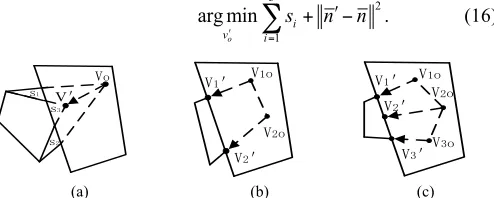
. (16)

Vo

V＇

s2 s1

s3

V1o

V1＇

V2＇ V2o

V1o V1＇

V3＇

V2o

V3o V2＇

[image:10.612.50.297.318.417.2]

(a) (b) (c)

Fig. 14. Three cases of mesh face structure that should be deformed: (a) one vertex under front view surface; (b) two vertices under front view surface; and (c) three vertices under front view surface.

Fig.14 (b) and (c) show the other two cases respectively with two and three vertices in the mesh face belonging to the

occluded surface. Let the occluded vertices be denoted by ,

where . The vertices in the occluded mesh face and

the corresponding face above them are projected onto the X-Y

plane to get two closed polygons and . Let denotes the

curve that intersects the two closed polygons. The newly

transformed occluded vertices are denoted by which are

located within curve and the updated face retains the same

normal vector _{that satisfies} .

Step 2) Obtain the partial ROI surface between

β

and θ

using the initial ROI surfaces of the front view part denoted by

PF

Yθ _and

GF

Yβ_{. Let}

R

α→β denote the 3D rotation transformation

matrix from view

_α

to view

β

. The initial ROI surfaces are

affine transformed by Y_PFθ R

θ→β

⋅ and YGFβ ⋅Rβ→θ . They are

transformed to each other’s view. Step 1 is repeated on the two surfaces to remove the new occluded vertices. Finally, transform the resulting partial similar surface to the same view. The gait partial ROI elements are then denoted by

,

₍

₎

ROI G

Ga

<β θ>

Y

β _and ,

_{( )}

ROI P

Pr

<β θ>

Y

θ _{that set}

G

Y

β _and

P Yθ

respectively as the gallery ROI and probe ROI.

2) Partial gait energy image (PGEI)

An incomplete binary silhouettes is the projection of the common view surface and is composed of gait partial ROI

elements denoted by ,

ROI

Ga

<β θ> _and ,

ROI

Pr

<β θ>_{. By using the}

partial ROI elements, the partial similar surface meshes can be

represented. Transforming them to the same galleryβview,

and projecting to X-Y space form 2D partial images denoted

by ,

, ( , )

Ga t

I<β θ> x y _and ,

, ( , )

Pr t

I<β θ> x y _{. The partial similarity gait}

energy images is

, , 1 , , , 1

1 _{( , ),}

( , ) 1 ( , ) N Ga t t M Pr t t

I x y Gallery N

PGEI x y

I x y Probe R R OI OI M β θ β θ β θ < > = < > < > = ⎧ ⎪ ⎪ =_⎨ ⎪ ⎪ ⎩

∑

∑

(17)

whereβis the gallery view andθthe partial destination view.

IV. ARBITRARY-VIEW GAIT RECOGNITION BASED

ON MULTI-LINEAR SUBSPACE ANALYSIS To realize arbitrary-view gait recognition with partial similarity matching, a synthetic database with destination

views is constructed based on GPSM. Let

_β

₀

₌

_β

_G be the

gallery view and

β

_N+₁

=

β

_p be the probe view. Let

{

1, n, , N

}

ϕ

∈

β

K

β

K

β

be the synthetic destination views. The

training partial similarity matching features are denoted by

(

)

(

)

(

)

(

)

(

)

(

)

(

)

(

)

(

)

0 0 0

1 1 1 1 1 1 , , , , , , , , , G

G G G

G G G

N

m M

m

G N G N G

M

m M

Y Y Y

D Y Y Y

Y Y Y

ϕ ϕ ϕ

β

ϕ

β β

β β

β β

β β

β β

β β

β

+

β

β

+

β

β

+

β

⎡ ⎤ ⎢ ⎥ =⎢ ⎥ ⎢ ⎥ ⎢ ⎥ ⎣ ⎦ K K K K K K (18)

where

₍

,

₎

m _{, G}

G m

Y PGEI

ϕ

ϕ β β

β β

= < >, andMdenotes the number

of classification. Let

D

{

D

G

}

ϕ β

ϕ

=

, the synthetic database

D

ϕ

which is represented by a higher order tensor. Multi-linear subspace analysis has been shown to be good for analysing an ensemble of images [52]. We represent the gait PGEI features of different objects with multiple partial views as a

higher-order tensor D . The row of the tensor denotes the

PGEIs with the same partial view. The column of the tensor defines the PGEIs of the same objects. The longitudinal of the tensor illustrates the PGEIs of the different gallery views.

Tensors are multi-linear mappings over a set of vector

spaces. The order of tensor

A

_∈

R

I1× × × ×K In K IN isNelements of

Α are denoted as

1 n N

i× × × ×K i K i

A , where

1

≤

i

n

≤

I

n. The tensor D

is decomposed into different constituent factors by subjecting it to a generalization of N-mode single value decomposition that orthogonalizes the N spaces and decomposes the tensor as the mode-n product of N-orthogonal spaces. Thus a tensor can be expressed as a multi-linear model of factors as [52]

1 1 2 2 3 m n N N

×

×

×

K

×

×

=

U

U

U

U

D Z

. (18)

n o v 1, 2,3 n∈ o

D D_t l

n

vʹ′

l

nʹ′ arg min 2

n o v