warwick.ac.uk/lib-publications
Original citation:
Pollicott, Mark and Vytnova, Polina. (2016) Linear response and periodic points. Nonlinearity, 29 (10).
Permanent WRAP URL:
http://wrap.warwick.ac.uk/81577
Copyright and reuse:
The Warwick Research Archive Portal (WRAP) makes this work by researchers of the University of Warwick available open access under the following conditions. Copyright © and all moral rights to the version of the paper presented here belong to the individual author(s) and/or other copyright owners. To the extent reasonable and practicable the material made available in WRAP has been checked for eligibility before being made available.
Copies of full items can be used for personal research or study, educational, or not-for-profit purposes without prior permission or charge. Provided that the authors, title and full
bibliographic details are credited, a hyperlink and/or URL is given for the original metadata page and the content is not changed in any way.
Publisher’s statement:
This is an author-created, un-copyedited version of an article published in Nonlinearity. IOP Publishing Ltd is not responsible for any errors or omissions in this version of the manuscript or any version derived from it. The Version of Record is available online at
http://dx.doi.org/10.1088/0951-7715/29/10/3047
A note on versions:
The version presented here may differ from the published version or, version of record, if you wish to cite this item you are advised to consult the publisher’s version. Please see the ‘permanent WRAP URL’ above for details on accessing the published version and note that access may require a subscription.
1 INTRODUCTION
M. Pollicott1 and P. Vytnova2
1Mathematical Institute, University of Warwick, Coventry, CV4 7AL, UK
2School of Mathematical Sciences, Queen Mary University of London, Mile End Road, London E1 4NS, UK
E-mail: [email protected]
Abstract. Given an expanding map of the interval we can associate an absolutely continuous measure. Given an Anosov transformation on a two torus we can associate a Sinai–Ruelle–Bowen measure. In this note we consider first and second derivatives of the change in the average of a reference function. We present an explicit convergent series for these derivatives. In particular, this gives a relatively simple method of computation.
Submitted to: Nonlinearity
1. Introduction
Linear response can often be used to describe how physically relevant quantities respond to external stimuli. We recall the following informal description of Ruelle [14]: “Linear response theory deals with the way a physical system reacts to a small change in the applied forces or the control parameters. The system starts in an equilibrium or a steady stateρ, and is subjected to a small perturbation x, which may depend on time. In first approximation,
the change ∆ρ of ρ is assumed to be linear in the perturbation x”. A more mathematical
formulation is the following. Letf :M →M be a smooth discrete time dynamical system (on a compact Riemann manifoldM) admitting a unique SRB measure µ. Assume that λ7→fλ
is a smooth path throughf =f0 and that there exists a large enough set Λ, containing 0 as an accumulation point, so thatfλ admits an SRB measureµλ for each λ∈Λ. One asks how
smooth the map λ 7→µλ at 0, in particular whether it is differentiable (see [2]).
Ruelle presented explicit formulae for the first derivative (using the susceptibility function) in [15]. For example, if we associate a vector fieldX so thatfλ =f0+λX◦f+o(λ) then one can hope to write
∂ ∂λ
Z
gdµλ
λ=0 =
∞
X
n=0 Z
hX,grad(g◦f0n)idµ. (1.1) {susf:eq}
However, to make sense of this expression one needs, for example, that the right hand side of (1.1) converges in a suitable sense.
An approach suggested by Ruelle, was to consider the susceptibility function
Ψ(z) =
∞
X
n=0
zn
Z
1.1 Maps of the circle 1 INTRODUCTION
which reduces to (1.1) whenz = 1.
In an incomplete manuscript of Sondergaard and Cvitanovi´c, the authors propose the idea of studying this problem using a different approach involving a complex function defined using periodic orbits [8]. We want to develop further these ideas in the context of Cω
expanding maps and Anosov diffeomorphisms, a key point being the use of a somewhat different complex function. (A related problem was posed by Baladi in §5 in her survey [2], where she asked about the relationship of periodic points and linear response.) In particular, we present an alternative convergent series for the Right Hand Side of (1.1), which has the merit of being easily computed.
The problem of computing the first derivative of the integral was studied by Bahsoun and Galatolo [10]. Their proof takes a functional analytic approach by rewriting the Fr´echet derivative of the measure using transfer operators. Using approximation of the transfer operator by finite (although very large) rank operators, they obtain estimates on the derivative to any prescribed level of accuracy. This method has the distinct advantage that it applies to expanding maps of finite differentiability (for example, C3). By contrast, we require the stronger hypothesis that the map is real analytic, but then our proof involves deriving an alternative expression for the derivative in (1.1) as a series each of whose terms are defined in terms of weights on periodic points for the map. We require the strong analyticity hypothesis in order to ensure that this series converges and, moreover, sufficiently rapidly to give very good numerical approximations. In particular, this approach provides both good and effective estimates on the error, see Subsection 4.2. The advantage of this approach is numerical stability due to simplicity of the calculations involved. In particular, the algorithm presented in Section 4.1 can be realised on any pocket-sized calculator.
We consider the problem in the settings of expanding maps of the circle and Anosov diffeomorphisms of the torus. Our results are as follows.
1.1. Expanding maps of the circle
The simplest possible setting in which to study these problems is expanding maps of the circle.
Let us take a family ofCω expanding mapsT
λ :T1 →T1,λ∈(−ε, ε), on the unit circle
K =R/Z. We denote by
dµλ =ρλ(x)dx
the associated absolutely continuous invariant measure, with density ρ∈Cω(T1) [7]. Given a Cω function g : T1 → C we can consider the average R gdµλ, which has an analytic
dependence on λ ∈ (−ε, ε), and find an expression in terms of periodic orbits for the derivatives.
A = ∂
∂λ
Z
gdµλ
λ=0
and B = ∂ 2
∂λ2 Z
gdµλ
λ=0
1.2 Anosov diffeomorphisms 1 INTRODUCTION
In particular, this would lead to a series expansion
Z
gdµλ =
Z
gdµ0+λA+λ2
B
2 +o(λ 2
). (1.4) {avdif:eq}
The following theorem is our main result on expanding maps and gives both the desired expression for the coefficients in (1.3) in terms of periodic points and convergence estimates which will be useful later for computations.
{main1:thm} Theorem 1.1. LetTλ be a family ofCω expanding maps of the circle, letµλ be the absolutely
continuous invariant probability measure and let g be a Cω test function. Then
(i) The first and the second coefficientsA andB may be written as explicit convergent series
A=
∞
P
n=0
An and B = ∞
P
n=0
Bn;
(ii) The kth term of the series is defined in terms of periodic points of period ≤k;
(iii) The partial sumsSn(A) = n
P
k=1
Ak andSn(B) = n
P
k=1
Bk of the first n terms in each series
converge faster than any exponential to A and B, respectively, i.e., An ≤ αexp(−βn2)
and |Bn| ≤αexp(−βn2) for some α, β >0.
For clarity of exposition, we have formulated the result for expanding maps of the circle, but an extension to expanding maps in higher dimensions also holds.
Contributions to the study of this and related problems have been made by Ruelle [15] and [16], Baladi and Smania [3], [4], [5]; Dolgopyat [9], Liverani and Butterley [6].
The connection with periodic points is not unfamiliar, we recall
Lemma 1.2. The average of a test function is related to periodic orbits by the formula
Z
gdµλ = lim n→+∞
P
Tn
λxλ=xλg(x)· |T 0
λ(xλ)|−1
P
Tn
λxλ=xλ|T 0
λ(xλ)|−1
.
The rate of convergence in this lemma is typically only exponential, which is the same as the growth rate of the number of the periodic points needed to compute the terms.
However, our goal is to give an explicit convergent power series in λ, where the coefficients can be efficiently computed in terms of periodic points, as in Theorem1.1.
1.2. Anosov diffeomorphisms
We recall that a diffeomorphism f :M →M on a compact manifold is Anosov if
(i) there exists a continuous (in the manifold) Df-invariant splitting T M =Es⊕Eu and
constants C >0 and 0 < λ <1 such that kDfn|
Esk ≤ Cλn and kDf−n|Euk ≤Cλn for
n ≥0.
1.2 Anosov diffeomorphisms 1 INTRODUCTION
Let us consider a family of Cω Anosov diffeomorphisms f
λ : M → M, λ ∈ (−ε, ε). Let µλ
be the associated Sinai–Ruelle–Bowen measures. Given a Cω function g : M →
R we can consider the average R gdµλ, which has an
analytic dependence on λ ∈ (−ε, ε) and find an expression for its derivatives in terms of periodic orbits.
A= ∂
∂λ
Z
gdµλ
λ=0
and B = ∂ 2
∂λ2 Z
gdµλ
λ=0
In particular, this would lead to a series expansion, similar to (1.4)
Z
gdµλ =
Z
gdµ0+λA+λ2
B
2 +o(λ
2). (1.5) {
ava:dif}
The following theorem is our main result on Anosov diffeomorphisms and gives both the desired expression for the coefficients in (1.5) in terms of periodic points and convergence estimates which will be useful later for computations. Let us restrict to the case of Anosov diffeomorphisms of the two torus T2.
{main2:thm}
Theorem 1.3. Let Tλ be a Cω family of Anosov diffeomorphisms of T2, let µλ be the SRB
measures and let g be a Cω test function. Then
(i) The first and the second coefficientsA andB may be written as explicit convergent series
A=
∞
P
n=0
An and B = ∞
P
n=0
Bn;
(ii) The k’th term of the series is defined in terms of periodic points of period ≤k;
(iii) The partial sumsSn(A)
def =
n
P
k=1
AkandSn(B)
def =
n
P
k=1
Bk of the firstk terms in each series
converge faster than any exponential to A and B, respectively. In particular, there exist constants α, β > 0, which can be explicitely estimated, such that |An| ≤ αexp(−βn2)
and |Bn| ≤αexp(−βn2).
For clarity of exposition, we have formulated the result for Anosov diffeomorphisms of
T2 , but an extension to higher dimensional Anosov diffeomorphisms also holds.
We present the explicit formulae for the Sn(A) and Sn(B) in a later section.
The connection with periodic points is again well known:
Lemma 1.4. The average of a test function is related to periodic orbits by the formula
Z
gdµλ = lim n→+∞
P
Tn
λxλ=xλg(x)· |det(DTλ|E
u)(xλ)|−1
P
Tn
λxλ=xλ|det(DTλ|Eu)(xλ)| −1
The rate of convergence in this lemma is typically only exponential, which is the same as the growth of number of the periodic points needed to compute the terms. Thus Theorem1.3
1.3 Examples 1 INTRODUCTION
1.3. Examples
{numeric:sec} To illustrate the efficiency of the approach to numerical computation we can consider several
simple examples. We say that an estimateAN is accurate tok-decimal places we mean that
the sequence of approximations AN have the property that consecutive approximations AN
and AN+1 agree to k-places. Moreover, our approach does give explcit bounds, but they are not as sharp as the numerics suggest would be possible.
1.3.1. Expanding maps of the circle
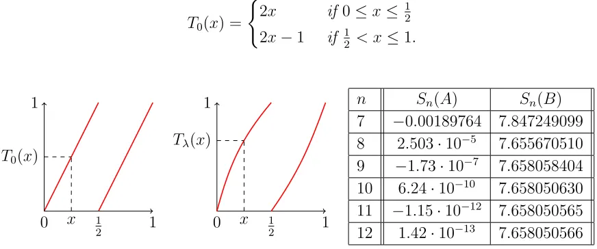
Example 1.5. Let T0 : [0,1]→[0,1] be the doubling map defined by
T0(x) = (
2x if 0≤x≤ 1 2 2x−1 if 12 < x≤1.
x T0(x)
1
0 1 1
2
x Tλ(x)
1
0 1 1
2
n Sn(A) Sn(B)
[image:6.612.85.521.246.428.2]7 −0.00189764 7.847249099 8 2.503·10−5 7.655670510 9 −1.73·10−7 7.658058404 10 6.24·10−10 7.658050630 11 −1.15·10−12 7.658050565 12 1.42·10−13 7.658050566
Figure 1. (a) The doubling map T0; (b) The small perturbation Tλ; (c) Approximations
to the first derivative and to the second derivatives. {conv:tab}
Let Tλ : [0,1]→[0,1] (−21π < λ < 21π) be the map defined by
Tλ(x) =
(
2x+λsin(2πx) if 0≤x≤ 1 2 2x−1 +λsin(2πx) if 12 < x≤1.
Let g(x) = cos(2πx). In this case the value A = 0 can be obtained as a part of general statement, outlined in the Appendix 4.3 p. 17, and this leads to a useful check on the numerics. In particular, using only ≈2000 periodic points with period ≤10 we see from Table 1 (a) accuracy to 9decimal places. Similarly, we have a method for finding numerical
approximations Bk toB = ∂
2
∂λ2
R
gdµTλ|λ=0 using periodic orbits of period ≤k. For instance,
using only ≈8000 periodic points with period ≤12 we get accuracy to 9 decimal places.
1.3.2. Anosov diffeomorphisms
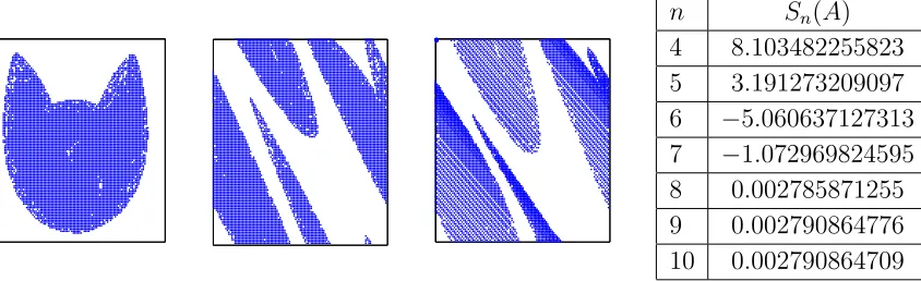
Example 1.6. We can consider the Arnol’d CAT map T0 :T2 →T2 given by
2 APPROACH OF THERMODYNAMICS
n Sn(A)
[image:7.612.87.509.77.206.2]4 8.103482255823 5 3.191273209097 6 −5.060637127313 7 −1.072969824595 8 0.002785871255 9 0.002790864776 10 0.002790864709
Figure 2. The case of Anosov diffeomorphisms. (1) Original domain (2) the image under
T0. (3) The image underTλ. (4) Approximations to the first derivative ∂λ∂ R gdµλ. {convan:tab}
and define a small perturbation
Tλ(x, y) = (2x+y+λcos(2πx), x+y) mod 1.
The number of periodic points of T0 grows exponentially like 3+
√ 5 2
n
, and they are
equidistributed. We need to choose test function changing rapidly in order to reduce
computational error. For example, one can considerg(x, y) = sin(19 sin(2πx) + 41 cos(2πy)). We obtainA= 0.00279. . .with≈6000periodic points of period9with accuracy to10decimal places.
2. Approach of thermodynamics
We will present the argument in a simple case of expanding maps and explain afterwards the changes needed in the case of invertible Anosov diffeomorphisms.
In this section we introduce determinants, which are complex functions whose zeros can be expressed in terms of a suitable thermodynamical pressure function. We will also recall that the integral of the test function which we study can be expressed in terms of a suitable derivative of this pressure. We are interested in the derivative of this integral as given in (1.1). So by the Implicit Function Theorem we will see that this can be expressed in terms of the derivatives of the determinant. This is the key to our approach.
2.1. Expanding maps of the circle
2.1 Expanding maps of the circle 2 APPROACH OF THERMODYNAMICS
2.1.1. Thermodynamic formalism LetT: T1 →
T1 be an expanding map on the unit circle.
We can consider the Cω function F :
T1 →R defined by
F(x) = −log|T0(x)|.
Definition 2.1. Leth(m) be the entropy of the measurem. We define the pressure function P :C(T1,R)→R by
P(F) := sup
m
h(m) + Z
F dm
where the supremum is over all T-invariant probability measures. Let µF be the Gibbs
measure associated to F, i.e.,
P(F) = h(µF) +
Z
F dµF
Let us consider an analytic family Fλ: T1 → T1 of expanding maps on the circle with
parameter λ∈(ε, ε) and denote µλ :=µFλ. The following result is well known [17].
{difP:lem}
Lemma 2.2. Let g :T1 7→
R be a real analytic function. Then the function t7→P(Fλ+tg)
is analytic and we can write
∂P(Fλ+tg)
∂t
t=0= Z
gdµλ
2.1.2. Determinant for the expanding maps We now introduce a complex-valued function
of three variables, associated to the familyFλ: T1 →T1 and a test functiong:T1 →C
Definition 2.3. The determinant d: C×R×(−ε, ε)→C, is a formally defined function
d(z, u, λ) = exp
−
∞
X
n=1
zn n
X
Tn λxλ=xλ
exp(−ugn(xλ)) |(Tn
λ)0(xλ)| −1
(2.1) {det:eq}
where the second summation is over periodic points xλ for Tλ of period n and we write
gn(x λ) =
n−1 P
k=0
g(Tk λxλ).
It is relatively classical to show the following.
{ancov:lem}
Lemma 2.4. For z ∈C, λ∈(−ε, ε) and u∈R we have that:
(i) d(z, u, λ) converges to an analytic function for |z|<exp(−P(Fλ−ug));
(ii) d(z, u, λ) has an analytic extension in z ∈C to the entire complex plane C;
2.1 Expanding maps of the circle 2 APPROACH OF THERMODYNAMICS
These results can be easily deducted from the paper of Ruelle [18] and his book [17], but we briefly recall the idea of the argument.
Let us treat the circle T1 as the unit interval [0,1]. Let [0,1] ⊂U ⊂
C be its complex
neighbourhood. We let B be the Banach space of bounded analytic functions f : U → C
with the supremum norm k · k∞.
{trop:def} Definition 2.5. To a family of maps Fλ ∈ B and a test function g ∈ B we associate the
transfer operator Lu,λ :B →B:
(Lu,λ)f(x) =
X
k
exp (Fλ−ug)(Tkx)
f(Tkx)
where Tk:U →U are Cω contractions with Tk(U)⊂U, and Tλ◦Tk is the identity map.
Providing that Fλ :U →C and u:U →Care analytic, the operators Lu,λ are nuclear.
In particular, the determinant
det(I−zLu,λ) = exp − ∞
X
n=1
zn
ntrace(L
n u,λ)
!
is an entire function in z. The previous statements come easily from results of Ruelle [18], after Grothendieck [11]:
{acoefs:lem} Lemma 2.6 (Grothendieck–Ruelle). We can expand the determinant in a power series
det(I − Lu,λ) = 1 + ∞
P
n=1
an(u, λ)zn, where the coefficients an satisfy: there exists α > 0
and 0< θ <1 such that |an(u, λ)| ≤αθn
2 .
In particular, we see the following
{z0:cor}
Corollary 2.7. Let z =z(u, λ) be the real zero for d(z, u, λ), i.e. d(z(u, λ), u, λ) = 0. Then z(0, λ) = 1 for all λ ∈(−ε, ε).
Proof. By Rohlin’s equality we have thatP(Fλ) = 0 for all λ∈(−ε, ε).
Using Lemma 2.2 we can observe
∂
∂λz(u, λ) = ∂
∂λexp(−P(Fλ−ug)) =−z(u, λ) ∂
∂λP(Fλ−ug)
2.1.3. Analytic dependence of the average on measure Implicit to our analysis is that the
function λ 7→ R
gdµλ is analytic in λ, from which we can then turn to the problem of
solving the derivatives. This is part of a general result whereby we consider analyticity of the determinant d(z, u, λ), defined by (2.1). We may introduce an analytic function
η: C×(−ε, ε)→C by
η(z, λ) := ∂logd(z, u, λ)
∂u
u=0 = 1
d(z, u, λ)
∂d(z, u, λ)
∂u
u=0
=
∞
X
n=1
zn X
Tn λxλ=xλ
gn(x)
n
1
|(Tλn)0(x λ)|
2.2 Anosov diffeomorphisms 2 APPROACH OF THERMODYNAMICS
Lemma 2.8. The function η(z, λ) has a simple pole at s= 1 with residue R
gdµλ.
For each individual periodic pointTn
λ(xλ) =xλ we have aCω function (−ε, ε)3λ7→xλ.
Moreover, we can find a common neighbourhood (−ε, ε) ⊂ U such that (−ε, ε) 3 λ 7→ xλ
has an analytic extension to U.
Lemma 2.9. In a neighbourhood 1 ∈ V ⊂ C we have that V 3 z 7→ η(z, λ)−1 is analytic. Moreover, U 3λ7→η(z, λ)−1 ∈Cω(V,C) is also analytic.
Recall Corollary 2.7. We can use the residue theorem to deduce that
U 3λ7→ 1
η(z, λ) 7→ Z
gdµλ
is analytic.
2.2. Anosov diffeomorphisms
Let T: T2 →
T2 be an Anosov diffeomorphism of the torus, i.e. we assume that there
exists a DT-invariant splitting T2 =Es⊕Eu, and C, ρ >0 such that
DTn|Es
≤Cρn and
DT−1|Eu
≤Cρn. We also assume that the map T has a dense orbit.
We will begin by reviewing thermodynamic formalism for Anosov maps of the torus. This then allows us to describe the zeros of the complex determinant function we need to introduce. We also include a brief description of the Banach space and operators (due to Rugh) that we use.
2.2.1. Thermodynamic formalism We can consider the H¨older functionϕu: T2 →Rdefined by
ϕu(x) =−log|det(DxT|Eu)|
and theCω function ϕ:
T2 →R given by
ϕ(x) =−log|det(I−DT)|
Definition 2.10. We define the pressure function P :C(T2,R)→R by
P(T) := sup
m
h(m) + Z
T dmT
where the supremum is over allT-invariant probability measures. LetµT be the Gibbs measure
associated to T, i.e., the unique T-invariant probability measure such that
P(T) = h(µT) +
Z
T dµT.
Let Tλ: T2 → T2 be a family of Anosov diffeomorphisms. Let ϕuλ and ϕ s
λ be the
2.2 Anosov diffeomorphisms 2 APPROACH OF THERMODYNAMICS
{difP2:lem} Lemma 2.11. Let w:T2 7→R be a real analytic function. The function t 7→P(−ϕλ+tw)
is analytic and we can write
∂P(ϕλ+tw)
∂t
t=0= Z
wdµλ,
where µλ is the SRB measure and P(ϕuλ) = 0.
2.2.2. Determinant for Anosov diffeomorphisms We recall the result of Rugh from [19].
For a real analytic Anosov diffeomorphismT :T2 →T2 and a positive real analytic function
g :T2 →
R+ given by g(z) = exp(w(z)) we can associate the function
d(z)def= exp − ∞
X
n=1
zn
n
X
Tnx=x
Qn−1
k=0g(T
kx)
det(DTn(x)−I)
!
.
which converges for |z|<exp(P(−φu+w)). In particular, we observe that
lim
n→+∞
exp
n−1 P
k=0
φu(Tkx)
det(DTn(x)−I) = 1. (7.1)
We have the following interpretation.
Proposition 2.12 (Rugh). The function d(z) has an analytic extension to C with a simple zero at z = exp(P(−φu+w)).
However, examining the proof we see that there is an additional analytic dependence. We therefore define
d(z, s, λ) := exp
−
∞
X
n=1
zn
n
X
Tn λxλ=xλ
exp
sPn−1
k=0w(T
k λx)
det(DTn
λ(x)−I)
. (2.3) {det2:eq}
Lemma 2.13 (Ruelle–Grothendieck–Rugh). The function d: C×R×(−ε, ε) → C, given by (2.3) is analytic. Furthermore, we can write
d(z, s, λ) = 1 +
∞
X
n=1
an(s, λ)zn
where there exists 0< θ <1 such that such that |an(s, λ)|=O(θn
2
).
Thus the truncations
d(N)(z, s, λ) = 1 +
N
X
n=1
an(s, λ)zn
are efficient approximations to d(z, s, λ) and lead to approximations to R wdµλ via the
2.2 Anosov diffeomorphisms 2 APPROACH OF THERMODYNAMICS
Example 2.14. We can consider the Arnol’d CAT map T0 :T2 →T2 defined by T0(x, y) = (2x+y, x+y) (mod 1). We can then define Tλ(x, y) = (2x+y+λsin(2πx), x+y). The
periodic points for T0 correspond to (xx12) = (A
n−I)−1(n
m) where n, m∈Z, and A = (2 11 1).
2.2.3. The Banach spaces and transfer operators of Rugh For completeness, we briefly recall the approach by Rugh.
The spaces constructed by Rugh in his paper [19] were the forerunners of the modern theory of Anisotropic Banach spaces. For our purposes, the most important feature is that it retains the property of being a nuclear space.
One associates to the Anosov map a Markov partition P = {P1,· · · , Pk}. Each piece
of the partition can be written in the form [Ui, Si] where Ui ⊂Wu(zi) and Si ⊂Wu(zi), for
somezi ∈Pi, and we write [x, y] =Ws(x, ε)∩Ws(y, ε) for sufficiently smallε >0, depending
only on T. Following the original work of Adler and Weiss [1], and Sinai [20], we can model
T: T2 →
T2 by a subshift of finite type σ: ΣA→ΣA with transition matrix A.
On each piece Pi of the partition one can consider the natural coordinates associated
to the stable and unstable manifolds (i.e., we can identify points in Pi with Ui ×Si using
the above. As is well known, these coordinates are typically only C1. In order to recover analytic coordinates we need to use an approach introduced by Rugh.
Assume that z0 ∈ Pi0, T z1 ∈ Pi1. In particular, writing z0 = (x0, y0) and z1 = (x1, y1)
we see that for each
(i) y0 ∈Ui0 the map x0(·, y0) :Si1 →Si0 is an analytic contraction.
(ii) x1 ∈Si1 the map y1(x1,·) :Ui0 →Ui1 is an analytic expansion.
Here contraction and expansion are understood in terms of the modulus of derivative being smaller, or larger, than 1 respectively.
By virtue of real analyticity, we can fix small neighbourhoods Si0 ⊃ Si0 and Ui1 ⊃ Ui1
with smooth boundaries corresponding to complexifications of these pieces of unstable and stable maps such that:
(i) for anyy0 ∈ Ui0 the mapx0(·, y0) :Si0 → Si1 is an analytic contraction and, in particular,
x0(Si0, y)⊂ Si1.
(ii) for anyx1 ∈ Si1 the mapsy1(x1,·) :Ui1 → Ui0 is an analytic expansion and, in particular,
y1(x1,Ui1)⊂ Ui0.
(iii) We can solve yj(ξ0, φs(ξ0, η1)) = η1 to get a family of contractions φs(ξ0,·) :Ui1 → Ui0
(indexed by ξ0).
(iv) We define a family of contractions φu(·, η1) : Si0 → Si1 by φu(ξ0, η1) = y1(φs(ξ0, η1))
(indexed by η1).
We can consider the space of functions B :=⊕iCω(Si×(bC− Ui)) consisting of bounded
analytic functions f : `
3 DETERMINANT AND TEST FUNCTION
operator L:B →B by
Lf(x1, y1) = − X
A(i0,i1)=1
1 4π2
Z
∂Si Z
∂Ui
f(x0, y0)·G(x1, y0)
(x0−ϕu(x0, y1))(y1−ϕs(x0, y1))
dx0dy0
where A is the transition matrix, (x0, y0) ∈ Si0 × (bC − Ui0) (x1, y1) ∈ Sj × (bC − Uj),
and G(x0, y1) = ∂2φs(x0, y1) is a weight function associated with the change of variables (cf. Rugh [13]).
3. Determinant and test function
The coefficientsAandB, defined by (1.3), can be written in terms of the determinant. They give linear and quadratic approximations to the derivative of the average (1.4). We keep the notation introduced in the previous section.
The first coefficient A may be written in a relatively easy closed form.
{difD:lem}
Lemma 3.1 (Linear approximation).
A= ∂
∂λ Z gdµλ λ=0 =−
∂2d(1,u,λ)
∂u∂λ |u=0,λ=0 ∂d(z,0,0)
∂z |z=1
! +
∂2d(z,0,λ)
∂z∂λ |z=1,λ=0
∂d(1,u,0)
∂u |u=0
∂d(z,0,0)
∂z |z=1
2
.
Proof. By the implicit function theorem applied to d(z(u, λ), u, λ) = 0 we can write
−
∂d(z(0,λ),u,λ)
∂u
u=0
∂d(z,0,λ)
∂z
z=z(0,λ)
= ∂z(u, λ)
∂u
u=0
=z(0, λ)∂P(Fλ−ug)
∂u
u=0
= ∂P(Fλ −ug)
∂u
u=0
, (3.1) {difD1:eq}
using the corollary 2.7 to see that z(0, λ) = 1, and by Lemma 2.2
∂P(Fλ−ug)
∂u u=0 =− Z
gdµλ. (3.2) {difD2:eq}
We thus see from the two identities (3.1) and (3.2) that
Z
gdµλ =−
∂d(z(0,λ),u,λ)
∂u
u=0
∂d(z,0,λ)
∂z
z=z(0,λ)
.
Differentiating with respect to λ and taking into account that ∂z∂λ(0,λ)
λ=0= 0, we get the result.
The expression for the second coefficient B = ∂λ∂22
R
gdµλ
λ=0 involves third-order
derivatives of the determinant. {B:lem} Lemma 3.2 (Quadratic approximation).
B =∂d
∂z
−1 ∂3d
∂u∂2λ−
∂3d
∂u∂λ2 −
∂3d
∂z∂λ2· Z
gdµ0−2
∂2d
∂z∂λ·A− ∂2d
∂z2 ·A· Z
gdµ0
u=0,λ=0,z=1
,
where A= ∂λ∂ R
gdµλ
3.1 Differentiating determinant 4 NUMERICAL RESULTS
Proof. To estimate the value B we differentiate the determinant twice, and calculate
∂2
∂λ2
∂
∂ud(z(u, λ), u, λ))|u=0
|λ=0 using the identities z(0, λ)≡0 and ∂z∂λ(0,λ
λ=0= 0.
It is clear therefore that in order to estimate the coefficientsA and B, it is sufficient to be able to compute efficiently derivatives of the determinant. Below we provide theoretical background and outline computational method.
3.1. Derivatives of d(z, u, λ)
Since the determinant is an analytic function, we can expand it in a power series.
d(z, u, λ) = 1 +
∞
X
n=1
an(u, λ)zn. (3.3) {dets:eq}
Comparing the terms in the expansion for d(z, u, λ) given by (2.1) we get the following.
{anest:lem}
Lemma 3.3. Let g : T1 →
R be real analytic, and let Tλ: T1 → T1 be a family of the
expanding maps of the circle. Then each an(u, λ) depends only on periodic points of period
n, i.e.,
an(u, λ) =
X
n1+···+nr=n
1
r!
r
Y
j=1
1
nj
X
Tnjxλ=xλ
exp(−ugnj(x)) (Tnj
λ )0(xλ)−1
Moreover, in the case of the doubling map on the circle, we can take any 12 < θ <1and then α can be explicitly estimated in the upper bound|an| ≤αθn
2 .
{anap:lem}
Lemma 3.4. The derivatives of the determinant (2.1) can be approximated by the sums of derivatives of coefficients an. Moreover, an upper bound for the approximation error can be
explicitly calculated.
4. Numerical results
We begin with an outline of the algorithm we use for computing the first and second derivatives of the integrals. We then illustrate this, firstly, for expanding maps of the circle and then, secondly, for Anosov diffeomorphisms of the torus.
4.1. Outline of the algorithm
{ss:algorithm}
Our expression for the first derivative of the integral from Lemma 3.1 together with Lemma 3.4 provides the basis for an efficient algorithm for estimating the numerical value of the derivative (1.1).
To present the algorithm used, we will need the following simple technical result.
{recc:lem}
Lemma 4.1. In notation introduced above, consider the values
bn(u, λ)
def
= X
Tn λ(xλ)=xλ
exp(−ugn(x λ)) |(Tn
λ)0(xλ)| −1
4.1 Outline of the algorithm 4 NUMERICAL RESULTS
Then the coefficients of the series (3.3) satsify the reccurent relation
an(u, λ) =−
1
n
n−1 X
j=0
aj(u, λ)bn−j(u, λ) (4.2) {mainrec:eq}
where a0 = 1.
Proof. We recall the determinant identity, that follows from (2.1) and (2.3)
exp
−
∞
X
n=1
zn
n
X
Tn λxλ=xλ
exp(−ugn(x λ)) |(Tn
λ)0(xλ)| −1
= 1 +
∞
X
n=1
znan(u, λ);
With notation introduced, it can be rewritten as
exp− ∞
X
n=1
zn n bn
= 1 +
∞
X
n=1
znan(u, λ);
The Lemma follows by induction in n. Differentiating n times both sides of the latter equation in z and evaluating the result at z = 0 we obtain the required relation.
Our algorithm is the following.
Step 1 FixN. We can compute the periodic points of the mapT0(for example, using iterations of the inverse transformation) up to period N and associate the values bn(u, λ) defined
by (4.1) as well as partial derivatives ∂bn
∂u, ∂bn
∂λ and ∂2bn
∂u∂λ. (We would like to stress out
that in order to avoid round-off errors, we calculate the derivatives analytically for each combination of perturbation and test function g.)
Step 2 We can derive the expressions for an (1 ≤ n ≤ N) in terms of bn (1 ≤ n ≤ N) using
reccurent relation (4.2).
Step 3 We can define approximations
dN(z, u, λ) = N
X
n=1
znan(u, λ)
to dN(z, u, λ). The derivatives of d(z, uλ) that appear in the formula in (3.1) can be
approximated by the derivatives of dN(z, u, λ) which take an explicit form:
∂2dN(z, u, λ)
∂u∂λ =
N
X
n=1
zn∂
2a
n(u, λ)
∂u∂λ
∂dN(z, u, λ)
∂λ∂z =
N
X
n=1
nzn−1∂an(u, λ) ∂λ
∂dN(z, u, λ)
∂u =
N
X
n=1
4.2 Convergence estimates 4 NUMERICAL RESULTS
∂dN(z, u, λ)
∂z =
N
X
n=1
nzn−1an(u, λ)
Step 4 We obtain partial derivatives of an involved in the formulae above using reccurent
relation (4.2), using derivatives of bn obtained in Step 1.
Step 5 We define subsequent approximations
AN :=−
∂2dN(z,u,λ)
∂u∂λ ∂dN(z,u,λ)
∂z
! +
∂dN(z,u,λ)
∂λ∂z
∂dN(z,u,λ)
∂u ∂dN(z,u,λ)
∂z
!2
In particular, we need only sum expressions involving the derivatives of the coefficients
an(u, λ) constructed in Step 4. It follows from Lemma 3.1 that
AN −→
∂ ∂λ
Z
gdµλ
λ=0
asN → ∞.
In the next subsection we provide an estimate on the rate of convergence.
4.2. Convergence estimates
{ss:convest} The rate at whichAN converges toA us controlled by the size of the discarded tail (fromN
to infinity) of the series.
To illustrate the approach, consider the case of real analytic expanding mapTλ : [0,1]→
[0,1] with λ ∈ (−ε, ε). We denote the inverse branches by Tλ,j : [0,1] → [0,1], with
j = 1,· · · , k. Let us assume that each Tλ,j has an analytic extension to a neighbourhood
B(x, r)⊃[0,1] for λ∈V, a bounded complex neighbourhood of x such that
∪jTλ,jB(x, r)⊂B(x, θ
1 2r)
for some 0< θ12 <1. Let us assume thatu∈U, a bounded complex neighbourhood ofx. We
can then boundanusing the approach in the proof of Lemma2.6 given in [18] (see also [12])
|an(u, λ)| ≤ kLu,λkn∞nn/2θ n
2, n ≥0,
where we use the supremum normkLu,λk∞for the operatorLu,λ acting on bounded analytic
functions on B(x, θ12r) with respect to the supremum norm.
The additional analytic dependence on λ and u is important to us in order to use Cauchy’s theorem to bound the derivatives of an(u, λ). In particular, we can write
∂an(u, λ)
∂u
u=0 = 1
2πi
Z
|ξ−1|=ρ0
an(ξ, λ)dξ
(ξ−1)2
for any ρ0 >0 such that B(0, ρ0)⊂U. Similarly,
∂an(u, λ)
∂λ
λ=0 = 1
2πi
Z
|ξ|=ρ1
an(u, ξ)dξ
4.2 Convergence estimates 4 NUMERICAL RESULTS
for any ρ1 >0 such that B(0, ρ1)⊂V. Finally, we can also write
∂2an(u, λ)
∂u∂λ
u=0,λ=0=− 1 (2π)2
Z
|ξ−1|=ρ0
Z
|η|=ρ1
an(ξ, η)dξdη
(ξ−1)2η2 .
In particular, we have
∂an(u, λ)
∂u u=0 ≤ 1 ρ2 0
kLu,λknnn/2θ
n
2
∂an(u, λ)
∂λ λ=0 ≤ 1 ρ2 1
kLu,λknnn/2θ
n
2
∂2a
n(u, λ)
∂u∂λ
u=0,λ=0 ≤
1
ρ0ρ1
kLu,λknnn/2θ
n
2
Bounds on error in approximation for the doubling map. We would like to give explicite
estimates in the cases we studied in Examples 4.3 and 4.4. Assume that Tλ(x) =
2x+λcos(2πx) (mod 1) and g(x) = sin(2πx).
We want to consider the case of a small λ 6= 0. Let Tb1,λ,Tb2,λ : C → C be defined by Tb1,λ(x) = 2x+λcos(2πx) and Tb1,λ(x) = 2x+λcos(2πx) + 1. We can choose r > 1 2 and then consider the images ∩jTbj,λ B 12, r
. We also require thatTj,λ are bijections from
B 12, r onto the image. We would then like to choose R > r and |λ| sufficiently small that
∩jTbj,λ B 12, r
⊃B 12, R. In particular, we can choose any
R <2r− 1
2− |λ| · kcos(2πx)k∞
where the supremum is over the diskB 12, r. We can trivially bound this bykcos(2πx)k∞≤
exp(2πr). We can then choose any
θ12 = r
R ≥
2r
4r−1−2λexp(2πr)
For example, if we choose R= 2, r = 32, and λ <exp(2πr) 2− 1 2r
, then we can choose any θ > 169 .
We next want to bound the norm of the operator Lλ,u acting on bounded analytic
functions on B 12,2 with respect to the supremum norm. In addition let us choose
|u| ≤ρ1 = 1001 . Directly from Definition 2.5 we deduce an upper bound
kLλ,uk ≤2k(Tλ)−1k∞exp
√ e5 100 ≤ 200
200−√e5 exp √ e5 100 ,
since for z ∈B 12,2 we have bounds|sin(2πz)|<√e5 and |cos(2πz)|<√e5.
Finally, using the above estimates we can explicitly bound the tail of the series for the derivatives, i.e., the difference between the derivatives for d(z, λ, u) and dN(z, λ, u), which
4.3 Some rigorous values 4 NUMERICAL RESULTS
4.3. Some rigorous values
{ap2} In the case of expanding maps of the circle, there is a nice criteria for estimating a linear
approximation to the average R gdµ, which is of independent interest.
{Aexpr:thm} Theorem 4.2. Assume that Tλ and g are chosen so that there exist a constant C0 and a
polynomial P0 such that for any n
1
|(Tn
0)0| −1 ·
X
Tn λ(xλ)=xλ
∂ ∂λ(T
n λ)
0
(xλ)
λ=0
≤P0(n) (4.3) {hyp1:eq}
1
n
X
Tn
0(x)=x
gn(x)
≤C0 (4.4) {hyp2:eq}
then
∂ ∂λ
Z
gdµλ
λ=0 = lim
n→∞
1
n ∂2
∂u∂λbn(u, λ)
u=0,λ=0
; (4.5)
where bn(u, λ) are sums over periodic orbits given by (4.1), providing the latter limit exists.
The hypothesis of Theorem 4.2 are satisfied; in particular, in the examples we will consider below. The second condition (4.4) holds true for any test function g with zero average R gdµ= 0.
Proof. The argument is very straightforward. The conditions (4.3) and (4.4), imposed on the diffeomorphism and the test function, allows one to show, relying on the analyticity of the determinant, that ∂d(1∂u,u,0)
u=0= 0 and
∂2
∂u∂λd(1, u, λ)
u=0,λ=0=
∂
∂zd(z, u, λ)
z=1,u=0,λ=0·nlim→∞
1
n ∂2
∂u∂λbn(u, λ)
u=0,λ=0.
Theorem follows from Lemma 3.1.
4.4. Expanding maps of the circle
Using the method described above, one can calculate partial derivatives of the first 16 coefficients a1, . . . , a16 very rapidly.
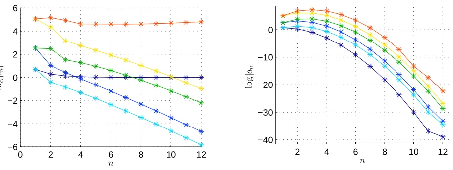
{ex:4.3} Example 4.3 (Tλ(x) = 2x+λcos(2πx) and g(x) = sin(2πx)). The left graph in Figure 3
shows a plot of sums over periodic orbits, bn and its derivatives against n in logarithmic
scale. We observe that log(bn) = ln(1 + 2n1−1) ≈ 1
2n−1 converges to 0, as it should, and
each of partial derivatives are asymptotic to exp(−αn) for some constant α > 0. The right graph in Figure 3 shows a plot of the Taylor series coefficients an and their derivatives
4.5 Anosov diffeomorphisms of the torus 4 NUMERICAL RESULTS
0 2 4 6 8 10 12
−6 −4 −2 0 2 4 6 n lo g | bn |
2 4 6 8 10 12
[image:19.612.72.529.81.253.2]−40 −30 −20 −10 0 n lo g | an |
Figure 3. Representative plots. On the left hand side we see the plot of sums |bn| (dark
blue) and partial derivatives∂b∂un (blue),
∂b∂λn
(light blue), ∂ 2b n ∂u∂λ (green), ∂ 2b n ∂λ2 (yellow),
and ∂ 3b
n
∂u∂2λ
(red) in logarithmic scale. On the right, the corresponding derivatives ofanare
shown. All derivatives are evaluated atλ= 0,u= 0. {sin2cos2:fig}
sums Sn(A) and Sn(B), approximating the coefficients A and B, respectively, were given in
Table 1. In this example we obtain
∂ ∂λ Z gdµλ
λ=0= 0; and
∂2 ∂2λ
Z
gdµλ
λ=0= 7.6505. . .
{ex:4.4}
Example 4.4 (Tλ(x) = 2x+λcos(4πx) and g(x) = sin(4πx)). Increasing the frequency
of perturbation and test function, we observe that for the second order partial derivative
log∂
2b
n
∂u∂λ
u=0,λ=0 6→ 0, and, consequently, we get
∂ ∂λ R gdµλ
λ=0= 1.570796326. . .; which
corresponds to the value π2 from Theorem 4.2 up to an error 10−12.
These estimates took only 7 seconds on a modern Desktop computer.
Example 4.5 (Tλ(x) = 2x + λcos(2πx) and g(x) = cos(2πx)). In this example we
consider synchronised perturbation and test function. As a result, we observe that one of the derivatives ∂an
∂λ
λ=0,u=0 vanishes, but log ∂ 2b n ∂u∂λ
u=0,λ=0 6→0, and we obtain
∂ ∂λ R gdµλ
λ=0= 1.570796326. . .; which corresponds to the value π2 from Theorem 4.2 up to an error 10−14.
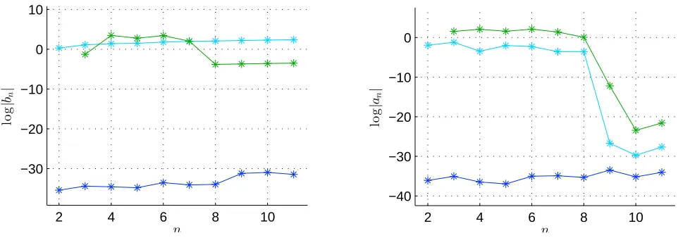
4.5. Anosov diffeomorphisms of the torus
It is well known that for an Anosov diffeomorphism A the total number of periodic points of period n is equal to det(An − I), therefore we see that bn(0,0) ≡ 1 for all n, and
d(z,0,0) = 1−z, i.e. a0(0,0) = 1, a1(0,0) =−1, and an(0,0) = 0 for all n 6= 1,2. Using
a similar method with obvious adjustments, we calculate partial derivatives of the first 10 coefficients a1, . . . , a10 of the Taylor series expansion of the determinant (2.3), evaluated at
λ= 0, u= 0. The Figure4shows the plots of sums over the orbitsbn and the coefficientsan
5 GENERALIZATIONS
2 4 6 8 10 −30
−20 −10 0 10
n
lo
g
|
bn
|
2 4 6 8 10 −40
−30 −20 −10 0
n
lo
g
|
an
[image:20.612.57.538.83.252.2]|
Figure 4. Representative plots. On the left hand side we see the plot of partial derivatives
∂b∂un
(blue),
∂b∂λn
(light blue), and
∂
2b n
∂u∂λ
(green) in the logarithmic scale. On the right,
the corresponding derivatives ofan are shown. All derivatives are evaluated atλ= 0,u= 0. {anosov:fig}
5. Generalizations
Finally, we formulate generalizations of Theorem 1.1 and Theorem 1.3 which can be proved with the same basic method.
We begin by considering the generalization of Theorem 1.1 to expanding maps on d -dimensional compact manifolds.
Theorem 5.1. Let Tt be a Cω family of expanding maps on a d-dimensional compact
manifold, let µTt be the absolutely continuous invariant probability measure and let g be
a Cω test function. Then
(i) The first and the second coefficients A and B may be written as explicit convergent series
A=
∞
P
n=0
An and B = ∞
P
n=0
Bn;
(ii) The kth term of the series is defined in terms of periodic points of period ≤k;
(iii) The partial sumsSn(A) = n
P
k=1
Ak and Sn(B) = n
P
k=1
Bk of the first k terms in each series
converge faster than any exponential to A and B, respectively, i.e., |An| ≤ αe−βn
1+1/d
and |Bn| ≤Ce−Bn
1+1/d
for some α, β >0.
Finally, we have generalization of Theorem 1.3 to Anosov diffeomorphisms on d -dimensional compact manifolds.
Theorem 5.2. LetTtbe aCω family of Anosov diffeomorphisms, letµft be the SRB measures
and let g be a Cω test function. Then
(i) There are expressions for A =
∞
P
n=0
An and B = ∞
P
n=0
Bn in terms of explicit convergent
6 REFERENCES
(ii) The kth term of the series is defined in terms of periodic points of period ≤k;
(iii) The partial sums Ak and Bk of the first k terms in each series converge faster than any
exponential to A and B, respectively.
Remark 5.3. The method we have described might also be be applied to Cω expanding
semi-flows and Anosov flows, by using Markov sections.
6. References
[1] R. L. Adler and B. Weiss. Similarity of automorphisms of the torus. Memoirs of the American Mathematical Society, No. 98 American Mathematical Society, Providence, R.I. 1970 ii+43 pp. [2] V. Baladi. Linear response despite critical points. Nonlinearity 21 (2008), no. 6, T81–T90.
[3] V. Baladi and D. Smania. Linear response for smooth deformations of generic nonuniformly hyperbolic unimodal maps. Ann. Sci. ´Ec. Norm. Sup´er. (4) 45 (2012), no. 6, 861–926 (2013).
[4] V. Baladi and D. Smania. Corrigendum: Linear response formula for piecewise expanding unimodal maps. Nonlinearity 25 (2012), no. 7, 2203–2205.
[5] V. Baladi and D. Smania. Alternative proofs of linear response for piecewise expanding unimodal maps. Ergodic Theory Dynam. Systems 30 (2010), no. 1, 1–20.
[6] O. Butterley and C. Liverani. Smooth Anosov flows: correlation spectra and stability. J. Mod. Dyn. 1 (2007), no. 2, 301–322.
[7] P. Collet and J.-P. Eckmann. Iterated maps on the interval as dynamical systems. Reprint of the 1980 edition. Modern Birkh¨auser Classics. Birkh¨auser Boston, Inc., Boston, MA, 2009. xii+248 pp. [8] P. Cvitanovi´c. Periodic orbit formulation of linear response. (working notes for N. S¨ondergaard) cf.
http://www.cns.gatech.edu/ predrag/papers/unfinished.html.
[9] D. Dolgopyat. On differentiability of SRB states for partially hyperbolic systems. Invent. Math. 155 (2004), no. 2, 389–449.
[10] W. Bahsoun, S. Galatolo, I. Nisoli, and X. Niu. A Rigorous Computational Approach to Linear Response. cf. http://arxiv.org/abs/1506.08661
[11] A. Grothendieck. Produits tensoriels topologiques et espaces nucl´eaires. Mem. Am. Math. Soc. 16. (1955) [12] O. Jenkinson and M. Pollicott. Calculating Hausdorff dimensions of Julia sets and Kleinian limit sets.
Amer. J. Math. 124 (2002), no. 3, 495–545.
[13] H. H. Rugh. The correlation spectrum for hyperbolic analytic maps. Nonlinearity, 5 (1992), 1237–1263. [14] D. Ruelle. A review of linear response theory for general differentiable dynamical systems. Nonlinearity
22 (2009), no. 4, 855–870.
[15] D. Ruelle. Differentiation of SRB states. Comm. Math. Phys. 187 (1997), no. 1, 227–241.
[16] D. Ruelle. Correction and complements: ”Differentiation of SRB states” Comm. Math. Phys. 234 (2003), no. 1, 185–190.
[17] D. Ruelle. Thermodynamic formalism. The mathematical structures of equilibrium statistical mechanics. Second edition. Cambridge Mathematical Library. Cambridge University Press, Cambridge, 2004. xx+174 pp.
[18] D. Ruelle. Zeta-functions for expanding maps and Anosov flows. Invent. Math. 34 (1976), no. 3, 231–242. [19] H. H. Rugh. Generalized Fredholm determinants and Selberg zeta functions for Axiom A dynamical
systems. (English summary) Ergodic Theory Dynam. Systems 16 (1996), no. 4, 805–819.