Fast Estimation of Range and Bearing for a Single Near-field Source without Eigenvalue Decomposition

Fast Estimation of Range and Bearing for a Single

Near-field Source without Eigenvalue

Decomposition

Hao Chen, Zhaohui Wu, Lu Gan, Xiaoming Liu, and Jinji Ma

Abstract—In this paper, a fast range and bearing estima-tion method for a single near-field source is proposed. By constructing the covariance matrix of received data, the phase containing the information of range and the direction of arrival is extracted. Finally, the phase is rewritten as matrix form, and the closed-formed solution of range and bearing of the source can be calculated by least square method. In contrast to high-order statistics based methods, the proposed method can obtain the range and bearing estimation without eigenvalue decomposition and spectral search, which remarkably reduce computational complexity. Simulation results show the proposed method can provide improved estimation accuracy and higher efficiency.

Index Terms—Estimation of range and bearing, single source, near-field, linear antenna array.

I. INTRODUCTION

E

STIMATION of range and bearing using array of sen-sors plays an important roles in microphone array, radar, sonar, and navigation. Uniform linear array is commonly used for target localization and allow for many fast esti-mation methods. However, the fast estiesti-mation methods are majority designed for far-field scenario, which the sources are located far from the array and the range of all sources is infinity. For the near-field sources , the sources are located close to the array, and the received data is a coupling of the direction of arrival (DOA) and range, the source localization is more complicated than the far-field scenario [1][2]. Therefore, the fast estimation methods are no longer applicable.

Many algorithms have been developed for range and bearing estimation of near-field sources, which can be mainly grouped into two categories. On one hand, there are spectral search based methods, especially the multiple signal clas-sification (MUSIC) [3] based methods . Two-dimensional (2-D) MUSIC algorithm was utilized to near-field multiple source localization, which can achieve a sufficiently good localization performance [4]. For a spherical microphone array, spherical harmonics 2-D MUSIC was also developed

Manuscript received October 15, 2018. This work was supported in part by the National Natural Science Foundation of China (No. 41671352 and 61871003), the Natural Science Foundation of Anhui province, China (No. 1708085QF133), and Natural Science Program of Universities in Anhui Province (KJ2017A329).

H. Chen is with the College of Physics and Electronic Information, Anhui Normal University, Wuhu, 241002 China. He is also with the Department of Neuroscience, Georgetown University, Washington D.C., 20007 USA. e-mail: [email protected].

Z. Wu, L. Gan, and X. Liu are with the College of Physics and Electronic Information, Anhui Normal University, Wuhu, 241002China.

[image:1.595.352.498.196.303.2]

J. Ma is with the College of Geography and Tourism, Anhui Normal University, Wuhu, 241002 China.

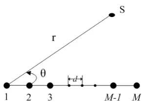
Fig. 1: Near-field ULA configuration.

[5]. However, the computational complexity is tremendous due to the 2D spectral search. To cope with this problem, covariance approximation MUSIC (CA-MUSIC) [6], sym-metric partition based MUSIC [7], and two-stage MUSIC [8] were developed, in which using twice one-dimensional (1-D) spectral search to substitute the 2-D search and reducing the computational burden. To some extent, these algorithms can reduce the computational complexity. However, twice 1-D spectral search and the eigenvalue decomposition implemen-tation still consume great compuimplemen-tational burden. Reduced-dimensional MUSIC algorithm for near-field sources was proposed recently [9], which can obtain the angle estimation by only 1-D search. On the other hand, high-order estima-tion of signal parameters via rotaestima-tional invariance technique (ESPRIT) algorithms are proposed, such as the second-order based method [10], four-second-order based method [11], and simplified high-order estimation (SHOE) method [12]. In [11], a four-order cumulant based total least square ESPRIT (TLS-ESPRIT) method was proposed for passive localization of near-field sources. High-order based algorithms always accompany with ESPRIT, hence eigenvalue decomposition is inevitable and increasing the computational complexity. In the SHOE, localization for near-field sources can be achieved based on the four-order cumulant and twice 1-D spectral search MUSIC, which is still time consuming.

In order to reduce computational burden, a fast estimation of range and bearing method is developed for a single near-field source. Neither spectrum search nor the eigenvalue decomposition operation is carried out in the proposed al-gorithm, which can reduce the computational complexity to a great extent. By constructing a correlation function based on the array configuration, the proposed algorithm provides a closed-form solution of the range and bearing based on the least square approach. In addition, the phase ambiguity is also considered. Compared with the SHOE and TLS-ESPRIT algorithm, the proposed algorithm can achieve better estimation accuracy and higher efficiency.

IAENG International Journal of Applied Mathematics, 48:4, IJAM_48_4_18

II. SIGNAL MODEL

As illustrated in Fig. 1, a single narrowband near-field source impinging on a uniform linear array (ULA) with M identical sensors, in which the distance between two adjacent elements isd and(θ, r)denotes the DOA and range of the source. The received data at themth sensor can be given by

xm(l) =s(l)ejψm_{+wm(l) (1)}

where l = 1,2,· · · , L, and L is the number of snapshots, s(l) is the source signal, wm(l) is the additive Gaussian white sensor noise,ψmis the phase shift between the signal received by the first sensor and the m sensor. In near-field scenario,ψmcan be denoted as [13]

ψm= 2πr

λ

r

1 +m

2_d2

r2 −

2mdsinθ

r −1

!

(2)

where λ is wavelength. For the source is in the Fresnel region, which is satisfying 0.62(D3

λ)1/2 _{< r < 2D}2

λ, with D is the array aperture, by applying the second-order Taylor expansion, the phase difference can be expressed as

ψm≈ −2πdsinθ

λ m+

πd2cos2θ

λr m

2_{+O d}2

r2

(3)

Neglecting the remainder termO d2r2of Taylor formula, ϕm can be written as

ψm=µm+δm2+O

_d2

r2

(4)

where

µ=−2πd

λ sinθ (5)

δ=πd

2

λr cos

2_{θ (6)}

Then, the received signal in Eq. (1) can be represented as

xm(l) =s(l)e j(−2πd

λ sinθ)m+j

πd2 λrcos

2_θm2

+wm(l) (7)

We make the following assumptions through this paper. 1) Impinging signal is circular. 2) The noise is independent from the source signal.

III. PROPOSED ALGORITHM

To estimate the DOA and range, a correction function is firstly constructed. The (p, q)th element in the covariance matrix of received data is

Rp,q =E[xp(l)x∗q(l)]

=ρ2_sej(−2πdλ sinθ)(p−q)+j

πd2 λr cos

2_θ

(p2−q2)_+ρ2

n (8)

where(·)∗ represents the complex conjugate,ρ2s andρ2n are the power of signal and noise, respectively. Due to there is only a single source in the near-filed, we extract the phase of Rp,q and obtain

σp,q=

−2πd λ sinθ

(p−q) +

_πd2

λr cos

2_θ

p2−q2

=−2πd λ

(p−q) sinθ− p2−q2 d

2rcos

2_θ

[image:2.595.305.546.72.314.2]

(9) It is known that the high direction finding accuracy can be obtained by large apertures. The lager apertures, the more

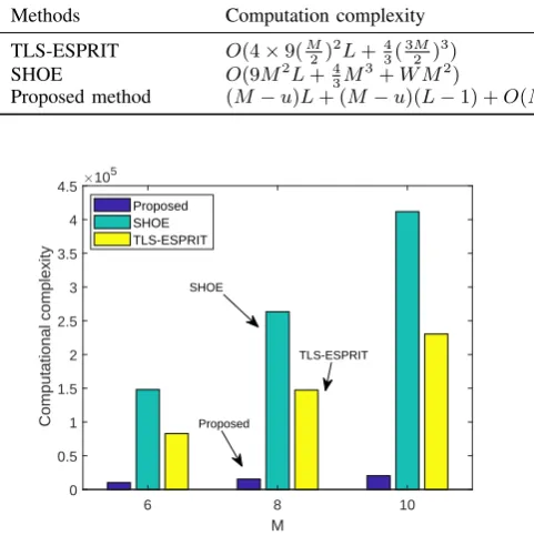
TABLE I: Computation complexity of the methods.

Methods Computation complexity

TLS-ESPRIT O(4×9(M

2 ) 2_L+4

3( 3M

2 ) 3₎

SHOE O(9M2_L+4

3M

3_{+W M}2₎

Proposed method (M−u)L+ (M−u)(L−1) +O(M)

6 8 10

M 0 0.5 1 1.5 2 2.5 3 3.5 4 4.5 Computational complexity 105 Proposed SHOE TLS-ESPRIT Proposed TLS-ESPRIT SHOE

Fig. 2: Comparison of the computation complexity.

accurate estimation. From Eq.(3), we can obtain whend > λ/2, there will be an ambiguity in the phase, which means that the phase difference is larger than2π. In this case, there will exist at least two direction of arrivals giving rise to the same received data. To guarantee there is no phase ambiguity inσp,q, it should satisfy the condition thatd/λ≤1/4. Note that the problem of phase ambiguity can also be solved by modulo conversion method [14]. Then, Eq. (9) can be express as

σp,q =−2πd λ

p−q q2−p2

T

sinθ d

2rcos

2_θ

(10)

where(·)T _{represents the transpose. Assume thatp−q=u,} we can express Eq. (10) in matrix form as

σ=ZB (11)

where

σ= [σ1,1+u, σ2,2+u,· · · , σM−u,M] T

(12)

Z=−2πd λ     

u (1 +u)2−12 u

.. . u

(2 +u)2−22 .. . M2−(M−u)2

     (13) B= sinθ d

2rcos

2_θ

(14)

Note that u is a constant, which can be chosen as

1,2,· · ·, M −1. To exploit the greatest degree of array aperture, we choseu= 2 in all of the simulations.

In practical, assumeRp,qˆ is the estimate ofRp,q, andˆσp,q is associated phase, by utilizing the least square method, the estimate ofBˆ can be obtained as

ˆ

B=hˆb1,ˆb2 iT

= ZTZ−1ZTσˆ (15)

IAENG International Journal of Applied Mathematics, 48:4, IJAM_48_4_18

[image:2.595.313.551.535.681.2]

where σˆ = [ˆσ1,1+u,σˆ2,2+u,· · ·,σˆM−u,M] T

. According to Eq. (14), θandrcan be estimated as

ˆ

θ= arcsin( ˆw1) (16)

ˆ r= dcos

2_θˆ 2 ˆw2

(17)

To analysis the estimation efficiency of the proposed method, we compare the computation complexity of the proposed algorithm with the TLS-ESPRIT based algorithm and the SHOE. As shown in Table 1, for a single source, the main computation load of the TLS-ESPRIT lies in construct-ing cumulant matrices and performconstruct-ing the EVD. Summconstruct-ing these two operations, the total computation load of the TLS-ESPRIT isO(4×9(M

2) 2_L+4

3( 3M

2 )

3_{). While for the SHOE,} twice 1-D spectrum search is needed. ForW points spectrum search, the total computation load of the SHOE is roughly O(9M2_L+ 4

3M

[image:3.595.323.523.179.338.2]

3_{+W M}2_{). In comparison, the proposed} algorithm needs neither constructing cumulant matrices nor performing the EVD, it only requires to formulate multiply operation in Eq. (8), and LS calculation in Eq. (15), and the total computation complexity is(M−u)L+(M−u)(L−1). Fig. 2 shows the computational complexity of the above three methods with L= 256, u= 2, and the search step is0.1◦, from which we can obtain that the proposed method has a much higher computational efficiency than the TLS-ESPRIT based algorithm and SHOE.

The advantages of the proposed method are as follow: 1) Without performing spectral search and eigenvalue de-composition, the proposed method has higher computational efficiency than the TLS-ESPRIT based algorithm and SHOE. 2) The proposed algorithm can provide closed-form solution of the range and bearing, and the has sufficiently good estimation accuracy.

IV. CRAMERRAO LOWER BOUND

The Cramer Rao lower bound (CRLB) is an important ref-erence to weigh the performance of an estimation algorithm. The inverse of the Fisher information matrix (FIM) is the CRLB, which bounds the error variance of the estimation from the radar system. According to the signal and system models, we can describe the FIM as

FIM= 2L σ2

n

Re DHΠ⊥_ADRT_S (18)

where D = [Dθ,Dr] with D(θ) =

∂A(θ,r)

∂r , D(r) = ∂A(θ,r)

∂θ , and A= [e

jψ1_,ejψ2_{,· · ·,e}jψM_]T_{. Moreover, Π}⊥

A =

I − A AHA−1AH, RT_S = SSHL, and S = [s(1), s(2),· · ·, s(L)]. DefineFindicates the FIM for target, which can be written as

F(θ, r) =

Fθθ Fθr

Frθ Frr

(19)

where

Ff,g= 2L σ2

n

n

Reh(D(f))HΠ⊥A(D(g))

RTS

io

(20)

and(f, g)∈ {θ, r}

V. SIMULATION RESULTS

In this section, several simulations are carried out to verify the performance of the proposed algorithm, which are also compared with the TLS-ESPRIT [11], the SHOE [12], and the CRLB [15]. For the simulations, a ULA with M = 9

and where K=500 is the number of Monte Carlo trials, xiˆ

is the estimated DOA or range of thekth trail, and xis the corresponding real value. d=λ/4is utilized, and the noise

25 27 29 31 33 35

DOA(degree)

1.5 2 2.5 3 3.5

Range/Lamda

Proposed method SHOE TLS-ESPRIT

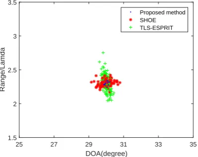
Fig. 3: Scatter plot forθ= 30◦ andr= 2.3λ.

−5 0 5 10 15 20 25 10−3

10−2 10−1 100 101

SNR(dB)

RMSE(degree)

[image:3.595.319.521.391.550.2]

Proposed method SHOE TLS−ESPRIT CRLB

Fig. 4: RMSE versus the SNR of DOA estimation.

−5 0 5 10 15 20 25 10−2

10−1 100 101 102

SNR(dB)

RMSE(wavelength)

[image:3.595.318.522.604.763.2]

Proposed method SHOE TLS−ESPRIT CRLB

Fig. 5: RMSE versus the SNR of range estimation.

IAENG International Journal of Applied Mathematics, 48:4, IJAM_48_4_18

100 300 500 700 900 1100 1300 1500 10−2

10−1 100 101

Number of snapshots

RMSE(degree)

[image:4.595.62.270.60.220.2]

Proposed method SHOE TLS−ESPRIT CRLB

Fig. 6: RMSE versus the number of snapshots of DOA estimation.

100 300 500 700 900 1100 1300 1500 10−2

10−1 100 101

Number of snapshots

RMSE(wavelength)

Proposed method SHOE TLS−ESPRIT CRLB

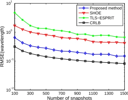
Fig. 7: RMSE versus the number of snapshots of range estimation.

is additive white Gaussian noise. A single source is located at(θ, r) = (30◦,2.3λ). We define the root mean square error (RMSE) of the estimate DOA and range as

RM SE=

v u u t

1 K

K

X

k=1

[image:4.595.318.521.61.219.2]

(ˆxk−x)2 (21)

Fig. 3 shows the scatter plot for L = 300, the signal-to-noise ratio (SNR) is 10 dB, the number of Monte Carlo is 200. We can obtain that the proposed methods holds a better localization accuracy than the TLS-ESPRIT method and SHOE.

As shown in Figs. 4 and 5, the RMSE of the DOA and range against the SNR, respectively. The number of snapshots is set asL= 300, and the SNR is varying from -5 to 25 dB. From these figures, we can see that the proposed algorithm has a lower RMSE than the SHOE and TLS-ESPRIT algorithm for both DOA and range estimation. Note that the estimate performance is distinctly enhanced at low SNR, which is ascribed to the proposed algorithm directly extract phase operation to restrain the influence of noise.

As depicted in Figs. 6 and 7, we analysis the RMSE of the DOA and range versus the number of snapshots. The SNR is fixed as 0 dB, and the number of snapshots is varying from 100 to 1500. For the DOA estimation, although the proposed

10 20 30 40 50 60 70 80 90

M

10-4 10-3 10-2 10-1 100 101

Run time(s)

Proposed method SHOE TLS-ESPRIT

Fig. 8: Run time versus the number of sensors.

algorithm exhibits similar RMSE to the SHOE, it is superior to that of the TLS-ESPRIT. For the range estimation, the RMSE of the proposed method is lower than that of the other two algorithms.

To demonstrate the computational efficiency, the simu-lation time of the proposed algorithm is compared with that of the SHOE and the TLS-ESPRIT. The number of snapshots is fixed at 256, and the SNR is 20, M = 10. The simulations are carried out at MATLAB platform with a PC of Inter(R) Core(TM) i5-4440 CPU and 8G RAM. The results are averaged over 500 runs. For the search interval is0.01◦, the computation consume of the SHOE, the TLS-ESPRIT, and the proposed algorithm are 0.3029, 0.0113, and

1.3879×10−4 _{s, respectively. The runtime versus sensor} number is depicted in Fig. 8, in which we can see that the proposed algorithm has much lower time consuming than the SHOE and the TLS-ESPRIT.

VI. CONCLUSION

A fast estimation of range and bearing algorithm is proposed for near-field source in this paper. To utilize the phase performance of received data for the single source, a correlation function matrix is constructed. The phase con-tains information about the range and DOA, which can be expressed as matrix multiply form. The closed-form solution of range and DOA can be obtained by least square method for the matrix. In addition, the CLRB of estimation is also derived. Compared with the TLS-ESPRIT and SHOE, the proposed method has higher accuracy and efficiency for escaping from spectral search and eigenvalue decomposition. Simulation results verify the performance advantages of the proposed method.

REFERENCES

[1] H. D. Noh and C. Y. Lee, “A Covariance Approximation Method for Near-Field Coherent Sources Localization Using Uniform Linear Array,”IEEE Journal of Ocearic Engineering, vol. 40, no. 1, pp. 187-195, Jan. 2015.

[2] K. Wang, L. Wang, J. R. Shang, and X. X. Qu, “Mixed near-field and far-field source localization based on uniform linear array partition,”

IEEE Sensor Journal, vol. 16, no. 22, pp. 8083-8090, Nov. 2016. [3] R. O. Schmidt, “Multiple emitter location and signal parameter

estima-tion,”IEEE Transactions on Antennas and Propagation, vol. TAP-34, no. 3, pp. 276-280, Mar. 1986.

IAENG International Journal of Applied Mathematics, 48:4, IJAM_48_4_18

[image:4.595.62.267.273.433.2]

[4] Y. D. Huang and M. Barkat, “Near-field multiple source localization by passive sensor array,”IEEE Transactions on Antennas and Propagation, vol. 39, no. 7, pp. 968-975, Jul. 1991.

[5] L. Kumar and R. M. Hegde, “Near-Field Acoustic Source Localization and Beamforming in Spherical Harmonics Domain,”IIEEE Transac-tions on Signal Processing, vol. 64, no. 13, pp. 3351-3361, Jul. 2016. [6] J. H. Lee, Y. M. Chen, and C. C. Yeh, “A covariance approximation method for near-field direction-finding using a uniform linear array,”

IIEEE Transactions on Signal Processing, vol. 43, no. 5, pp. 1293-1298, May 1995.

[7] W. Zhi and M. Y. W. Chia, “Near-field source localization via symmetric subarrays,”IEEE Signal Processing Letters, vol. 14, no. 6, pp. 409-412, June 2007.

[8] J. Liang and D. Liu, “Passive localization of mixed near-field and far-field sources using two-stage MUSIC algorithm,”IEEE Transactions on Signal Processing, vol. 58, no. 1, pp. 108-120, Jan. 2010. [9] X. F. Zhang, W. Y. Chen, W. Zheng, Z. X. Xia, and Y. F. Wang,

“Local-ization of near-field souces: a reduced-dimensiton MUCIS algorithm,”

IEEE Communications Letters, vol. 22, no. 7, pp. 1422-1425, July. 2018. [10] K. A. Meraim, Y. B. Hua, and A. Belouchrani, “Second-order near-field souce localization algorithm and performance analysis,” in Pro-ceesing of the 30th Asilomar Conference of Signals, System, and

Computer, Pacific Grove, pp. 723-727, CA, USA, Nov. 1997. [11] R. N. Challa and S. Shamsunder, “High-order subspace-based

algo-rithms for passive localization of near-field sources,” inProcessing of 29th Asilomar Conference on Signals, Systems, and Computers, Pacific Grove, CA, USA, Oct. 1995, pp. 777-781.

[12] J. Li, Y. Wang, C. L. Bastard, G. Wei, B. Ma, M. Sun, and Z. Yu, “Simplified high-order DOA and range estimation with linear antenna array,”IEEE Communnication Letters, vol. 21, no. 1, pp. 76-79, Jan. 2017.

[13] H. Chen, X. G. Zhang, Y. C. Bai, and J. J. Ma, “Computationally Efficient DOA and Range Estimation for Near-Field Source with Linear Antenna Array,” inProcessing of the World Congress on Engineering and Computer Science, 25-27 October, 2017, San Francisco, USA, pp: 412-415.

[14] K. R. Sundaram, R. K. Mallik, and U. M. S. Murthy, “Modulo conver-sion method for estimating the direction of arrival,”IEEE Transactions on Aerospace and Electronic Systems, vol. 36, no. 4, pp. 1391-1396, Oct. 2010.

[15] M. N. E. Korso, R. Boyer, A. Renaux, and S. Marcos, “Conditional and Unconditional Cramer Rao Bounds for Near-Field Source Localization,”

IEEE Transactions on Signal Processing, vol. 58, no. 5, pp. 2901-2907, Feb. 2010.

IAENG International Journal of Applied Mathematics, 48:4, IJAM_48_4_18