arXiv:1005.1536v1 [astro-ph.SR] 10 May 2010
Characterising Complexity in Solar Magnetogram Data using a
Wavelet-based Segmentation Method
P. Kestener
1, P.A. Conlon
2, A. Khalil
3, L. Fennell
2, R.T.J. McAteer
2, P.T. Gallagher
2and
A. Arneodo
4,51CEA, Centre de Saclay, DSM/IRFU/SEDI, 91191 Gif-sur-Yvette, France
2School of Physics, Trinity College Dublin, Dublin 2, Ireland
3Department of Mathematics&Statistics, The University of Maine, Orono, ME, USA 04469
4Universit´e de Lyon, F-69000, Lyon, France
5Laboratoire Joliot Curie and Laboratoire de Physique, Ecole Normale Sup´erieure de Lyon, 46 all´ee d’Italie, 69364
Lyon c´edex 07, France
ABSTRACT
The multifractal nature of solar photospheric magnetic structures are studied using the 2D wavelet transform modulus maxima (WTMM) method. This relies on computing partition functions from the wavelet transform skeleton defined by the WTMM method. This skeleton provides an adaptive space-scale partition of the fractal distribution under study, from which one can extract the multifractal singular-ity spectrum. We describe the implementation of a multiscale image processing segmentation procedure based on the partitioning of the WT skeleton which allows the disentangling of the information concerning the multifractal properties of active regions from the surrounding quiet-Sun field. The quiet Sun exhibits a average H¨older exponent∼ −0.75, with observed multifractal properties due to the supergranular struc-ture. On the other hand, active region multifractal spectra exhibit an average H¨older exponent∼ 0.38 similar to those found when studying experimental data from turbulent flows.
Subject headings: Sun: flares, Methods: statistical, data analysis, Techniques: image processing, Magnetic fields,
Turbulence
1. Introduction
Since the late 70’s and the propagation of fractal ideas throughout the scientific community (Mandelbrot 1982), there have been numerous applications of the concepts of scale invariance, self-similarity, long-range dependence in many areas of physics, chem-istry, biology, geology, meteorology, economy, so-cial and material sciences (Aharony & Feder 1989; West 1990; Vicsek et al. 1994; Bunde & Havlin 1994; Wilkinson et al. 1995; Family et al. 1995; Frisch 1995; Arneodo et al. 1995a; Bunde et al. 2002). Various methods were developed to quantify scale-invariance properties through the computation of the fractal di-mension DF for self-similar objects or the roughness
exponent H for self-affine fractals (Mandelbrot 1982; Peitgen & Saupe 1987; Feder 1988; Argoul et al.
1990; Lea-Cox & Wang 1993; Wilkinson et al. 1995; Taqqu et al. 1995). Unfortunately DF and H are
Grassberger et al. 1988). As to self-affine fractals, Parisi and Frisch (Parisi & Frisch 1985) proposed, for the analysis of fully-developed turbulence ve-locity data, an alternative multifractal description based on the investigation of the scaling behavior of the so-called structure functions (Frisch 1995; Monin & Yaglom 1975): Sp(l) =< (δvl)p >∼ lζp (p
integer> 0), whereδvl(x) =v(x+l)−v(x) ∼lh(x) is an increment of the recorded signal over a distance l. Then, after reinterpreting the roughness exponent as a local quantity (Parisi & Frisch 1985; Muzy et al. 1991, 1994; Arneodo et al. 1995c): δvl(x)∼lh(x)(power-law
behavior), the D(h) singularity spectrum is defined as the Hausdorffdimension of the set of points x where the local roughness (or H¨older) exponent h(x) of v is h. In principle, D(h) can be attained by Legendre transforming the structure function scaling exponents
ζp (Parisi & Frisch 1985; Muzy et al. 1991, 1994;
Arneodo et al. 1995c). Unfortunately, as noticed by (Muzy et al. 1991, 1993, 1994), both the box-counting and structure function methodology have intrinsic lim-itations and fail to fully characterize the corresponding singularity spectrum since only the strongest singular-ities are a priori amenable to these techniques. As such, both methods are limited in their application to real data sets (Muzy et al. 1994; Georgoulis 2005; Conlon et al. 2008).
In previous work, Arneodo and collaborators (Muzy et al. 1991, 1993, 1994; Arneodo et al. 1995c) have shown that there exists a natural way of performing a uni-fied multifractal analysis of both singular measures and multi-affine functions, which consists in using the
continuous wavelet transform (Goupillaud et al. 1984;
Grossmann & Morlet 1984; Meyer 1990; Daubechies 1992; Mallat 1998). By using wavelets instead of boxes, one can take advantage of the freedom of the choice of these “generalized oscillating boxes” to get rid of possible smooth behavior that might either mask singularities or perturb the estimation of their strength
h. The other fundamental advantage of using wavelets
is that the skeleton defined by the wavelet transform
modulus maxima (WTMM) (Mallat & Zhong 1992;
Mallat & Hwang 1992), provides an adaptative space-scale partitioning from which one can extract the D(h) singularity spectrum via the scaling exponentτ(q) of some partition functions defined from the WT skele-ton. The so-called WTMM method (Muzy et al. 1991, 1993, 1994; Arneodo et al. 1995c) therefore gives ac-cess to the entire D(h) spectrum via the usual Legendre transform D(h)=minq(qh−τ(q)). We refer the reader
to Bacry et al. (1993) and Jaffard (1997) for rigorous mathematical results and to Hentschel (1994) for the theoretical treatment of random multifractal functions. Applications of the WTMM method to 1D signals have already provided insight into a wide variety of problems (Arneodo et al. 2002), e.g. the validation of the log-normal cascade phenomenology of fully developed turbulence (Arneodo et al. 1998a, 1999b; Delour et al. 2001) and of high-resolution temporal rainfall (Venugopal et al. 2006a,b; Roux et al. 2009), the characterization and the understanding of long-range correlations in DNA sequences (Arneodo et al. 1995b, 1996; Audit et al. 2001, 2002), the demon-stration of the existence of a causal cascade of in-formation from large to small scales in financial time series (Arneodo et al. 1998b; Muzy et al. 2000), the use of the multifractal formalism to discrim-inate between healthy and sick heartbeat dynam-ics (Ivanov et al. 1996, 1999), the discovery of a Fibonacci structural ordering in 1D cuts of diff u-sion limited aggregates (Arneodo et al. 1992a,b,c; Kuhn et al. 1994) and in hard X-ray emission from so-lar fso-lares (McAteer et al. 2007). The WTMM method has been generalized from 1D to 2D with the spe-cific goal to achieve multifractal analysis of rough surfaces 1 with fractal dimension DF anywhere
be-tween 2 and 3 (Arrault et al. 1997; Arneodo et al. 2000; Decoster et al. 2000). The 2D WTMM method has been successfully applied to characterize the inter-mittent nature of cloud structure from satellite im-ages (Arneodo et al. 1999a; Roux et al. 2000) and to assist in the diagnosis of breast tissue lesions in digitized mammograms (Kestener et al. 2001). In astrophysics, this method was adapted and used to characterize the anisotropic structure of atomic hy-drogen gas (HI) in the Galatic disk (Khalil et al. 2006). From the analysis of very large mosaics taken from the Canadian Galatic Plane Survey (Taylor et al. 2003), directional roughness exponents were intro-duced to show that the HI in the Galactic spiral arms has a scale-dependent anisotropic signature while the HI in the inter-spiral arm regions exhibits scale-independent anisotropy. Along that line, the 2D WTMM method was further applied to char-acterize the space-scale nature of anisotropic struc-tures (Snow et al. 2008a,b; Khalil et al. 2009) and to perform objective segmentation of image features of
1The fractal dimension of a rough surface associated to the graph
z = S (x,y), where S (x,y) represents the height of the surface at
interest from noisy backgrounds (Khalil et al. 2007; Caddle et al. 2007; Roland et al. 2009). We refer the reader to Arneodo et al. (2003) for a review of the 2D WTMM methodology, from the theoretical con-cepts to experimental applications. Recently, the WTMM method has been further extended to 3D scalar (Kestener & Arneodo 2003) as well as 3D vec-tor (Kestener & Arneodo 2004, 2007) fields analysis and applied to 3D (velocity, vorticity, dissipation, en-strophy) numerical data issued from direct numerical simulations (DNS) of incompressible Navier-Stokes equations. Because it combines singular-value decom-position and multifractal description, the so-called ten-sorial wavelet transform modulus maxima method for vector fields (Kestener & Arneodo 2004, 2007) looks very promising for future simultaneous multifractal and structural (vorticity sheets, vorticity filaments) analysis of turbulent flows.
Our aim here is to exploit the ability of the WTMM method to study compound systems that dis-play some non-analyticity in their multifractal spec-tra as the signature of some phase spec-transition be-tween two underlying scale invariant components with different multifractal properties (Bohr & T`el 1988; Muzy et al. 1994; Arneodo et al. 1995c). These two components can both have some physical significance as previously experienced when using the WTMM method to detect vorticity filaments in swirling tur-bulent flows (Roux et al. 1999) or microcalcifications from breast tissue background in digitized mammo-grams (Kestener et al. 2001; Arneodo et al. 2003). One of these components can be noise that may cause drastic distortions in the returned multifractal spectra. In this work we will follow a wavelet-based strategy inspired from the one previously used in 1D to de-tect replication origins and promoters as jumps (dis-continuities) in 1D noisy skew profiles in mammalian genomes (Brodie of Brodie et al. 2005; Touchon et al. 2005; Nicolay et al. 2007) and in 2D to perform an objective and automatic segmentation of chromo-some territories in fluorescence microscopy imaging of mouse cell nuclei (Khalil et al. 2007; Caddle et al. 2007) and of gold formation on vapodeposited thin gold films (Roland et al. 2009).
The purpose of the manuscript is to demonstrate the suitability and reliability of the WTMM method to propose a wavelet-based segmentation procedure adapted to solar magnetogram data. In section 2, the basics of the 2D WTMM method are presented. Its ability to disentangle the underlying scale invariant
components of a compound system displaying a phase transition in its singularity spectra is discussed and a strategy of segmentation is implemented. Section 3 is devoted to a test application of the proposed segmen-tation procedure on a theoretical data set with known multifractal properties. In section 4 we report the re-sults obtained when using this wavelet-based segmen-tation method to separate active regions from quiet-Sun features in solar line-of-sight magnetogram data. Our conclusion and future directions are then given in Section 5.
2. Segmentation methodology of compound mul-tifractal systems using the 2D WTMM method
2.1. Basics of the 2D WTMM method
The main steps of the 2D WTMM method are pre-sented here. Details can be found in Arneodo et al. (2000); Decoster et al. (2000); Arneodo et al. (2003); Khalil et al. (2006).
1. Computation of the 2D continuous wavelet transform of the input image function f (x) with analyzing wavelets defined as the partial deriva-tives of a smoothing Gaussian kernelφ:
Tψ[ f ](b,a) =
Tψ1[ f ]=a−
2R
d2xψ1
a−1(x
−b)f (x) Tψ2[ f ]=a−
2R
d2xψ 2
a−1(x
−b)f (x)
,
= ∇{Tφ[ f ](b,a)} (1) = ∇{φb,a∗f},
whereψ1 = ∂φ/∂x, ψ2 = ∂φ/∂y and φ(x) =
exp(−|x|2/2). Eq. (1) amounts to define the 2D wavelet transform as the gradient vector of f (x) smoothed by a dilated version φ(a−1x) of the
Gaussian filter.
2. For each scale a, extract the WTMM edges de-fined as the locations b where the WT modulus
Mψ[ f ](b,a)=|Tψ[ f ](b,a)|is locally maximum
in the direction of the WT vector Tψ[ f ](b,a).
These WTMM points lie on connected maxima
chains. Along each of these maxima chains,
locate the local maxima called WTMMM for WTMM maxima. Note that the two ends of an open maxima chain are not allowed to be a pos-sible WTMMM location.
3. Extract the WT skeleton which is the set of
max-ima linesLx0obtained by connecting these
x0 at smallest scale. Start at the smallest scale
amin∼7pixels (minimum size of the support of the wavelet function) and link each WTMMM to their nearest neighbor found at the scale just above. Proceed iteratively from scale to scale up to the largest scale amax(limited by the
im-age size and border effects in wavelet transform computations). It is important to recall here that these lines contain all the information about the local H¨older regularity properties of the function
f under consideration and that along a maxima
lineLx0that points to x0in the limit a→0 +, the
wavelet transform modulus behaves as a power law:
Mψ[ f ][Lx0(a)]∼a
h(x0), (2)
where h(x0) is the H¨older exponent, i.e. the
strength of the singularity of the function f at the point x0.
4. From the WT skeleton compute the partition functions:
Z(q,a)= X
L∈L(a)
h
Mψ[ f ](x∈ L,a) iq
, (3)
which allows to define the τ(q) scaling expo-nents as
Z(q,a)∼aτ(q), a→0+. (4)
One can optionnally compute the companion partition functions h(q,a) and D(q,a) and
de-fine the corresponding scaling exponents when
a→0+
h(q,a)= P
L∈L(a)ln
Mψ[ f ](x,a)
Wψ[ f ](q,L,a) ∼a
h(q), (5)
D(q,a)= P
L∈L(a)Wψ[ f ](q,L,a) ln
Wψ[ f ](q,L,a)
∼aD(q).(6)
where
Wψ[ f ](q,L,a)= h
Mψ[ f ](x,a) iq
/Z(q,a) (7)
5. Compute theτ(q) spectrum by performing lin-ear regression fits of lnZ(q,a) vs ln a and finally
compute the D(h) singularity spectrum by Leg-endre transformingτ(q):
D(h)=min
q
qh
−τ(q). (8)
Alternatively D(h) can be computed from the es-timate of the scaling exponents h(q) and D(q) in Eqs. (5) and (6) respectively.
Note that alternative approaches to the WTMM method have been developed using discrete wavelet bases including the recent use of wavelet leaders (Jaffard et al. 2006; Wendt & Abry 2007; Wendt et al. 2007). We think that the continuous WT better suits our goal to provide a selective multifractal analysis of multi-component images via some objective segmentation of maxima lines in the WT skeleton.
2.2. Adapting the 2D WTMM method to the seg-mentation of compound multifractal systems
For simplicity, we will assume that the compound multifractal systems of interest here can be considered as the sum of two scale invariant components:
f (x)= fI(x)+fII(x) (9)
characterized by the singularity spectra DI(h) and DII(h) respectively. Ideally we will further suppose
that DI(h) and DII(h) have non-overlapping support
[hI min,h
I
max]∩[hIImin,h II
max] = ∅ and that hImax < hIImin
meaning that fI(x) possesses stronger singularities
than fII(x). In the limit a → 0+, the partition func-tionZ(q,a) (Eq. (3)) can be split into two parts:
Z(q,a)=ZI(q,a)+ZII(q,a)=CI(q)aτI(q)+CII(q)aτII(q),
(10) where CI(q) and CII(q) are prefactors that depend on q. Since hImax<hminII , it follows easily that in this limit, there exists a critical value qcritso that:
τ(q)= (
τI(q) for q>qcrit
τII(q) for q<qcrit (11)
Therefore, the τ(q) spectrum has a non-analyticity at
qcrit; when crossing this critical value, there is a
tran-sition from one scale invariant component to the other. As illustrated in Fig. 1, when Legendre transforming Eq. (11), one gets the upper envelop of the DI(h) and DII(h) spectra, a classical result for entropy in
equilib-rium statistical physics (Bohr & T`el 1988; Muzy et al. 1994; Arneodo et al. 1995c). In that respect the classi-cal 2D WTMM method does not provide separate ac-cess to DI(h) and DII(h).
Our segmentation strategy consists in using the WT skeleton to discriminate the maxima lines LI(a) as-sociated with singularities of fI(x) and maxima lines
LII(a) associated with singularities of fII(x), over the
range [amin,amax] of accessible scales. This can be
the WT skeleton (Eq. (2)). From the local estimate of h(x), one can expect to partition the WT skeleton into two sub-skeletons, one made of the maxima lines
LI(a) and the other one made of maxima lines
LII(a).
In practice, this partitioning will suffer from the finite range of scales available to the analysis and the de-sired segmentation will require special care as far as finite-size effects and statistical convergence issues are concerned.
3. Application of the wavelet-based segmentation method to synthetic data
We consider an academic example image with two fractal components: the fractal Dragon (Duda 2007) embedded into a noisy background generated from fractional Brownian noise with H¨older exponent H =
−0.7. The fractal Dragon is a self-similar fractal defined as the limit set of an iterated function sys-tem (the Lindenmayer syssys-tem) of the same type as the one used to generate the Sierpinski gasket or the Von Koch curve (Mandelbrot 1982), but the fractal Dragon has less obvious geometrical symmetries. Let us note that the fractal Dragon is space-filling, mean-ing its fractal dimension is 2, whereas its boundary has a fractal dimension known analytically DDragon =
log2(1+
3
√
73−6√87+√373+6√87
3 )≃1.5236. A sample
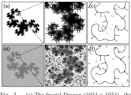
frac-tal Dragon is shown in Figure 2(a) whereas the corre-sponding noisy two-component image is shown in Fig-ure 2(d). As previously discussed, the wavelet analy-sis proposed in this work is sensitive to singularities,
i.e. to points in the images where the signal is
sin-gular. We expect the WTMM analysis of the image shown in Fig. 2(d) to simultaneously reveal multital information about both the boundary of the frac-tal Dragon and of the rough background texture. Let us recall that the two components have known mono-fractal type self-similar properties, i.e. a singularity spectrum degenerated to a single point: (h = −0.7,
D=2) for the fractional Brownian noise and (h=0,
D= DDragon ≃1.5236) for the boundary of the frac-tal Dragon. The roughness H =−0.7 of the fractional Brownian noise was chosen to mimic the texture of the quiet-Sun images (see Section 4.1). Figures 2(b) and 2(e) illustrate the results of the computation of the WT maxima chains at the smallest scale; the arrows corre-spond to the WT vectors (Eq. (2)) at the WTMMM lo-cations. Figures 2(c) and 2(f) show the maxima chains at a scale twice as large as in Figures 2(b) and 2(e). When going from large to small scales, whereas the
Fig. 1.— Illustration of a phase transition in the multifractal spectra of a compound system (Eq. (9)). (τI(q),DI(h)) and (τII(q),DII(h)) are the multifractal
spectra for fI(x) and fII(x) respectively. The 2D
WTMM method and more generally the multifrac-tal formalism, give access to the dashed τ(q) curve (Eq. (11)) in (a) and via the Legendre transform (Eq. (8)) to the dashed D(h) sprectrum in (b) which is the supremum of the DI(h) and DII(h) spectra.
Fig. 2.— (a) The fractal Dragon (1024×1024). (b) WTMM chains at the smallest scale a=σW =7
pix-els in a small 100×100 region of the fractal Dragon. (c) Same as in (b) for scale a = 2σW. (d) The
[image:5.612.330.508.137.213.2] [image:5.612.309.526.399.556.2]boundary of the fractal Dragon is better and better ap-proximated by some WTMM chains (edge detection in the smoothed image), an increasing number of addi-tional maxima chains start emerging as the signature of the presence of a colored noise (Fig. 2(e) as compared to Fig. 2(b)).
As previously emphasized (Muzy et al. 1994; Arneodo et al. 1995c, 2003), the set of maxima lines that defines the WT skeleton contains the space-scale information necessary to recover the underlying multifractal prop-erties. In Figures 3(a) and 3(b) are shown in a logarith-mic representation, the behavior of the WT modulus along the maxima lines computed for a noisy frac-tal Dragon with a noise amplitude respectively twice and five times as large as the fractal Dragon. Since the fractional Brownian noise is everywhere singular with H¨older exponent H = −0.7 (Mandelbrot 1982), maxima lines pointing to noise features at small scale are characterized by a WTMMM power law behavior
Mψ[ f ](a) ∼ a−0.7, while lines associated to the
frac-tal Dragon boundary can be distinguished by the fact thatMψ[ f ](a) ∼ a0 ∼Const (no scale dependence).
This leads us to implement the following segmenta-tion procedure: the space (log2a,log2Mψ[ f ](a)) is
divided in two regions separated by a straight line of slope−0.7<hs<0 and intercept log2Ms. As shown in Figure 3(a), for low noise amplitude, all the max-ima lines along which log2Mψ[ f ](a) decays slower
than hslog2a when increasing a, are colored in red
and associated with the Dragon boundary. On the con-trary, all the maxima lines along which log2Mψ[ f ](a)
decays faster than hslog2a when increasing a, are
colored in blue and associated with the noise com-ponent. But as shown in Figure 3(b), for large noise amplitude the distinction of the two sub-skeletons is much more tricky at small scales where some entan-gling is observed. We thus adapt the segmentation criteria towards the largest scales in fully analogy with a different but conceptually similar adaptation of the 2D WTMM segmentation method (Khalil et al. 2007). Each maxima line is characterized by a length,
i.e. its maximun scale amax and the WT modulus
Mψ[ f ](amax) at that scale. A given maxima line is said
to belong to the Dragon sub-skeleton, if it satisfies the following condition :
log2Mψ[ f ](amax)≥hslog2amax+log2Ms. (12)
In Figures 4(a) and 4(b) are reported the results of the computation of the partition functions for the frac-tal Dragon alone and its noisy version after applying
[image:6.612.311.509.115.185.2]Fig. 3.— Log-log plot of WT modulus along the skeleton maxima lines versus scale. Lines are colored according to the segmentation procedure (Eq. (12)) : fractal Dragon boundary (red) and fractionnal Brown-ian noise (blue). (a) Noisy fractal Dragon with a noise amplitude twice as large as the fractal Dragon (see Fig. 2(d)). (b) Noisy fractal Dragon with a noise am-plitude five times as large as the fractal Dragon. The dashed black line represents the segmentation condi-tion (Eq. 12).
Fig. 4.— Multifractal analysis of the fractal Dragon (◦) and of the noisy (H = −0.7) fractal Dragon (•) after applying the segmentation procedure (Eq. (12)). (a) h(q,a) vs log2a for different values of q; the solid lines correspond to linear regression fits over the range of scales a ∈ [20,24] σ
W (resp. [20.5,23.5] σW) for
the fractal Dragon (resp. the noisy fractal Dragon af-ter segmentation). The symbols () correspond to the
h(q = 0,a) partition function obtained for the noisy
fractal Dragon without any segmentation. (b) D(q,a)
vs log2a. (c)τ(q) vs q; the dashed horizontal line is the theoretical spectrumτ(q) = −1.5236 (∀q) of the
[image:6.612.310.528.332.472.2]the segmentation condition (Eq. (12)) with hs =−0.5
and log2Ms=−3.2. In Figure 4(a), the partition func-tions h(q,a) (Eq. (5)) of the noisy Dragon display a
well defined scaling behavior over 3 octaves (com-pared to 4 octaves for the original fractal Dragon), for a wide range of values of q∈[−2,3]. For negative q val-ues, at very small scales, the segmentation procedure fails to disentangle the two components due to the con-tribution from the noisy component with h(q)≃ −0.7. Nevertheless the gain in scaling is unquestionable as compared to the behavior of the h(q,a) partition
func-tions without segmentation (thein Fig. 4(a)).
With-out any segmentation the partition functions are a mix-ture of different scaling behaviors from which reliable quantitative information cannot be extracted. In Fig-ures 4(c) and 4(d) are shown the correspondingτ(q) and D(h) spectra. Despite some slight departure from monofractality for the segmented noisy fractal Dragon (that is also observed but to a lesser extent in the orig-inal fractal Dragon as the result of finite-size effects), one recovers a rather good estimate of the fractal di-mension DF =1.57±0.03 of the fractal Dragon
bound-ary. Furthermore, as reported in Figure 4(d), our seg-mentation procedure has proved to be very efficient to estimate separately the D(h) singularity spectra of both the fractal Dragon and the noisy background. This efficiency is illustrated in Figure 5 where a 3D (x,y,scale) space-scale visualization of the maxima
chains of the noisy Dragon prior (Fig. 5(a)) and after (Fig. 5(b)) segmentation clearly confirms the elimina-tion of noise-induced small scale features that would otherwise severely affect the multifractal analysis.
Fig. 5.— 3D visualization in the space-scale (x,y,scale) representation of the WTMM chains
com-puted from the image shown in Fig. 2(d) before (a) and after (b) the segmentation procedure (Eq. (12)). At each scale a, only the maxima chains containing at least one WTMMM belonging to the resulting WT skeleton are displayed.
4. Application of the wavelet-based segmentation method to Solar magnetogram data
Magnetic field measurements were obtained by the Michelson Doppler Imager (MDI) on the Solar and
Heliospheric Observatory (SOHO), which images the
Sun on a 1024×1024 pixel CCD camera through a series of increasingly narrow filters (Scherrer et al. 1995). The final elements, a pair of tunable Michel-son interferometers, enable MDI to record filtergrams with an FWHM bandwidth of 94 mÅ. In this paper, 96-minute magnetograms of the full disc were used, which had a pixel size of ∼2”. For the purposes of this work, a series of magnetograms have been ana-lyzed to examine the difference in fractal properties between quiet and active solar regions. A total of 29 magnetograms representative of the quiet Sun were taken from December 21 to December 22, 2006 and a similar series of 28 images representative of the ac-tive Sun were taken from October 27 to October 29, 2003. In the solar photosphere, the large magnetic Reynolds number (∼107
−109) means that magnetic
field lines will be advected with the flow of plasma (McAteer et al. 2009). This system naturally leads to self-similarity, suggesting a multifractal study is appropriate (Lawrence et al. 1993; Abramenko et al. 2002; McAteer et al. 2005). As already mentioned, previous method of calculating the multifractal proper-ties of solar magnetic features are dependent on image resolution, thresholding, and instrument sensitivity. The WTMM method calculates the multifractal spec-trum of solar magnetic features based on the distribu-tion of gradients within the image at various scales. As such, the WTMM multifractal parameters are less sen-sitive to changes in image resolution and instruments than traditional methods.
4.1. Quiet-Sun multifractal properties
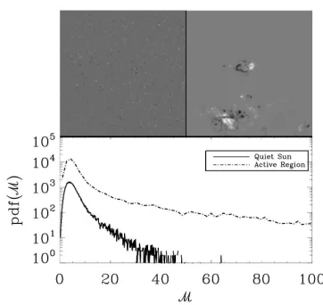
Examples of quiet and active MDI magnetograms analyzed are shown in Figure 6 (top left and top right respectively), with a histogram of the wavelet trans-form modulusMψ[ f ](b,a) at the smallest scale
mod-uli with values larger than 40 are unlikely in quiet-Sun magnetograms. Due to the different scaling properties of active regions and their surrounding quiet Sun, our goal is to segment the WT skeletons using the condi-tion defined in Eq. (12). As outlined in Seccondi-tion 2 and illustrated on synthetic data in Section 3, this should allow us to study the multifractal properties of active regions in a quantitative manner.
The results of the computation of the multifractal spectra when averaging the partition functions over a set of 30 (505×505) quiet-Sun images without ap-plying the segmentation are reported in Figure 7. As shown in Figure 7(a) and 7(b), h(q,a) (Eq. (5)) and D(q,a) (Eq. (6)) display convincing scaling behavior
over almost four octaves for q ∈[−2,3] (symbol (◦)). Linear regression fits of the data yield the non-linear
τ(q) spectrum shown in Figure 7(c). This multifractal diagnosis can also be observed in Figure 7(a) where the slope h(q) of the partition function h(q,a) versus
log2a definitely depends on q. The corresponding multifractal spectrum D(h) is shown in Figure 7(d). From the top of the D(h) curve, we can see that quiet-Sun images are everywhere singular (D(q = 0) = 2) with a corresponding H¨older exponent h(q = 0) ≃
−0.75. The multifractality can be quantified by the so-called intermittency coefficient c2that characterizes
the width of the D(h) curve. As shown in Figures 7(c) and 7(d), theτ(q) and D(h) data of the quiet-Sun im-ages are well fitted by a parabola
τ(q)=−c0+c1q−
c2
2q
2,
D(h)=c0−
(h−c1)2
2c2 ,
(13) where c0 ≃ 2, c1 ≃ −0.75 and c2 ≃ 0.22. Let us
point out that quadratic multifractal spectra are pre-dicted by the so-called log-normal model that has been popularized by the fully-developed turbulence com-munity (Frisch 1995; Arneodo et al. 1998a, 1999b; Delour et al. 2001). In the present case, there is no particular evidence of the relevance of this model ex-cept that the observedτ(q) and D(h) multifractal spec-tra are well characterized by their log-normal quadratic approximations.
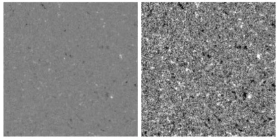
In order to understand the source of this intermit-tency, a upper threshold was imposed on each MDI magnetogram of the quiet Sun (Figure 8). The thresh-old operation has the effect of removing large magnetic features resting on the boundary of the super-granular structures of the Sun. In Figure 7(d), we can see that the multifractality of the thresholded quiet-Sun image (symbol) set is strongly reduced but not totally
can-Fig. 6.— (Top, Left) MDI magnetogram taken on December 20, 2006; (Top, Right) MDI magnetogram taken on October 28, 2003. (Bottom) Histogram val-ues of the wavelet transform modulusMψ[ f ](a) at the
smallest scale (σW =7 pixels) for MDI magnetogram
[image:8.612.324.505.116.287.2]images of a quiet Sun (solid) and active Sun (dashed).
Fig. 7.— Multifractal analysis of a set of 30 quiet-Sun images (505×505) prior (◦) and after () thresholding
(a sample thresholded magnetogram is shown in Fig-ure 8). (a) log2h(q,a) vs log2a for different values of q; the solid lines are linear regression fits over the range of scales a ∈ [20,23.7]σW. (b) log2D(q,a) vs
log2a. (c)τ(q) vs q; the dashed straight line is the theoretical linear spectrumτ(q) = −0.75q−2 of the 2D fractional Brownian noise with H¨older exponent
[image:8.612.310.527.399.545.2]celled. We can also note that the average H¨older ex-ponent is slightly shifted from<h >=c1 =−0.75 to
−0.82, and the intermittency coefficient is reduced to
c2 ∼ 0.06 (Let us recall that a value c2 = 0 means
that the underlying process is monofractal). With-out the super-granular magnetic structure, the quiet-Sun multifractal spectrum looks much more monofrac-tal. This suggests that the magnetic features rest-ing on the boundaries of the super-granular structure are a major actor in the observed intermittent struc-tural properties of the Sun (Georgoulis et al. 2002). Since current models for the solar dynamo use in-formation on the fractal dimension of solar disk as a whole (Pontieri et al. 2003), these new informations on the photosphere and the characteristic make-up of the quiet Sun should be incorporated in further theoretical works.
4.2. Solar magnetogram active region segmenta-tion
In this section, we highlight the use of the WTMM segmentation method on Solar magnetogram data with active regions, to demonstrate its ability to analyze the underlying multifractal properties of the active regions that are embedded in the surrounding quiet-Sun tex-ture.
A sample 505×505 magnetogram MDI image con-taining an active region is shown in Figure 9. Fig-ures 9(b) and 9(c) show respectively the results of the computation of the WTMM chains before and after the segmentation at scale a = σW ∼ 7 pixels of a small
[image:9.612.65.265.529.630.2]150×150 excerpt focused on the active location. As explained in Section 4.1, WT skeleton maxima lines
Fig. 8.— 256×256 quiet-Sun images. Image on the right is a threshholded version of the left one. Pixels with large absolute magnetic flux are shrinked down. Multifractal properties of quiet-Sun images and the corresponding thresholded versions are shown in Fig-ure 7.
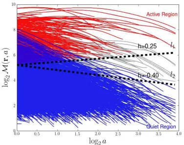
associated with quiet-Sun structures have a character-istic scaling behavior described byMψ[ f ](a)∼a−0.7.
This behavior is used to derive the parameters char-acterizing the line l2 in Figure 10 that will allow us
to discriminate in the WT skeleton, the maxima lines (blue) that correspond to quiet-Sun structures:
log2Mψ[ f ](amax)≤hQlog2amax+log2MQ, (14)
where−0.7<hQ<0, so that for the selected maxima lines log2Mψ[ f ](a) will decrease fast enough when
increasing the scale a to correspond to the quiet phase. To select the maxima lines (red) associated with the active region, we use another separating line l1in
Fig-ure 10:
log2Mψ[ f ](amax)≥hAlog2amax+log2MA, (15)
where this time 0 ≤ hA < 0.38, to limit the de-crease (if any) of log2Mψ[ f ] when increasing a. Note
that the lines l1 and l2 have different slopes because
some maxima lines cannot be clearly associated with either the quiet Sun or the active region state. In-deed those maxima lines are associated to features lo-cated near the boundary between quiet-Sun and ac-tive regions. When going from small scales to large scales the support of the analyzing wavelet starts cov-ering partly both regions preventing accurate classifi-cation. As illustrated in Figure 11, when fixing the segmentation parameters to hQ = −0.40, hA = 0.25
and log2MQ = log2MA = 5.2, the space-scale
na-ture of the methodology allows us to disentangle max-ima chains associated with the active region from those corresponding to the quiet Sun. Let us note that in a fu-ture work on large data sets, an automated parameters adjustment will be implemented using a clustering al-gorithm. In addition, a wrong choice of segmentation parameters can be observed in the partition function
Fig. 9.— (a) 505×505 Active Region example image (October 28, 2003). (b) WTMM chains at the smallest scale (a=σWpixels) in a small 150×150 region
[image:9.612.309.528.574.647.2]Fig. 10.— Log-log plot of the WT modulus along the skeleton maxima lines versus scale. The dashed line denoted l1 with slope hA = 0.25 and intercept
log2MA = 5.2 is used to identify WT skeleton max-ima lines associated to the active region (red). Ac-cording to Eq. (15), these lines have an ending point at highest scale (log2amax,log2Mψ[ f ](r,amax)) above
l1. The dashed line denoted l2with slope hQ=−0.40
and intercept log2MQ=5.2 is used to identify maxima lines associated to the quiet Sun (blue). According to Eq. (14), these lines have an ending point below l2. All
other lines (grey) are not clearly identified to belong either to the active site or the quiet surrounding. The values of the segmentation parameters hA, log2MA, hQ
and log2MQ were chosen by examining the WTMM
histogram at the smallest scale to extract at best a sub-skeleton specific to the active region.
plots (not shown here) which display a phase transition phenomenon, i.e. a scaling behavior that changes from one state to the other when going from small scales to large scale due to to non-homogenous phases and mis-classified maxima lines.
In Figure 12 are shown the results of the partition function computation for a set of 5 active region mag-netogram images taken on October 28th, 2003 (one
[image:10.612.67.255.234.382.2]image out of this set is shown in Figure 9(a)). Parti-tion funcParti-tions are computed separately for each sub-skeleton corresponding to the extracted action region maxima lines and quiet-Sun maxima lines shown in Figure 10. From these plots, one can see that the log2h(q,a) versus log2a data are nicely modeled with
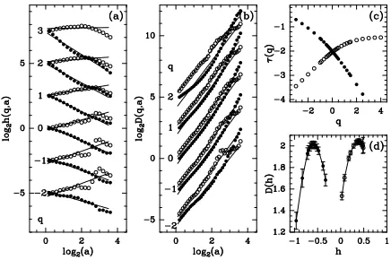
linear regression fits with slope h(q) that depends on q as the signature of multifractal scaling. This demon-strates that the segmentation procedure successfully extracts from the magnetogram images two scale in-variant components with different multifractal proper-ties. Theτ(q) (Fig. 12(c)) and D(h) (Fig. 12(d)) spectra computed from the set of quiet-Sun maxima lines (blue lines in Fig. 10) are in good agreement with the ones previously computed in Section 4.1 from pure quiet-Sun images (Figs. 7(c) and 7(d) respectively). Us-ing the log-normal approximation (Eq. (13)), we get
c0=2, c1=−0.65 and c2=0.10. This means that the
extracted quiet Sun appears (like the thresholded MDI magnetograms of quiet Sun in Figs 7(c) and 7(d)) a little less intermittent as compared to the previous es-timate c2 =0.22. As for the active region, the
corre-sponding partition functions computed from the set of active phase maxima lines (red lines in Fig. 10) dis-play very convincing multifractal scaling behavior as quantified by theτ(q) and D(h) spectra shown in Fig-ures 12(c) and 12(d) respectively. Again these spectra are well approximated by the quadratic log-normal for-mula (Eq. (13)) with parameters c0 =2, c1=0.38 and
c2 =0.12. This indicates that the singularities
associ-ated with the active region are space-filling (they are distributed on a set of fractal dimension DF =c0 =2),
with a mean strength h(q =0) =c1 =0.38 meaning
that magnetogram images can be considered as contin-uous on active regions (over the range of scales of our analysis) but noisy on quiet regions.
5. Conclusions
originat-Fig. 11.— 3D visualization in the space-scale (x,y,scale) representation of the WTMM chains
com-puted from the image shown in Fig. 9(a) before (left) and after (right) the segmentation procedure. The seg-mentation conditions are defined in Figure 10. The maxima chains displayed contain at least one WT-MMM belonging to the resulting skeleton.
ing from instrumental noise. As such these systems are a statistical combination of two distinct self-similar structures. This work addressed the need for an ac-curate calculation of the multifractal parameters of such complex systems. The presence of compound scale-invariant structures can result in an inaccurate or skewed calculation of the fractal and multifractal pa-rameters when studied as a whole. Using a wavelet-based multi-scale segmentation method, we show that it is possible to disentangle to some extent these two processes and accurately (up to finite-size effects) re-cover the multifractal characteristics of the system of interest. A theoretical test example for this method was provided in section 2. The removal of informa-tion relating to the background noise was highlighted in Figure 5. The quantitative results reported in Fig-ure 4 attest of the ability of this segmentation method to recover the multifractal parameters in question.
Let us emphasize here that the application of this method to experimental data for which we do not have a priori knowledge of the possible underlying multi-fractal processes is a difficult task that requires much attention to perform the most objective segmentation which can not be infered or guided by some physi-cal rule or information. The multifractal analysis is a statistical tool that has direct connections with sig-nal and image processing, but not necessarily with the physics of the system per se. As noticed in section 4.2, the use of a clustering algorithm should greatly help in adjusting the multifractal parameters of the diff er-ents componer-ents as well as in providing an automated procedure for processing large data sets. This will be reported in a future publication.
The application of this wavelet-based methodology to quiet-Sun data has revealed the multifractal nature of this intermittent noisy component (<h >=−0.75) as mainly resulting from the super-granular magnetic structures. The quiet-Sun study was also necessary to get expertise for further analyzing more complex images that involve a segmentation before being able to clearly identify the underlying multifractal proper-ties. We have checked that the partition functions com-putations for the segmented quiet-Sun phase provide (i) convincing scaling properties and (ii) multifrac-tal spectraτ(q) and D(h) estimates in good numerical agreement with the one measured in the previous cal-ibration step. The assumption of two non-overlapping
D(h) is not inconsistent with the data. Let us notice
segmenta-tion parameters are chosen. In the case of overlapping
D(h), there would be a large set of maxima lines in
the WT skeleton that could not be genuinely sorted, which would prevent from building accurate multifrac-tal D(h) measurement. From the analyzed data, we were not able to distinguish more than two phases. Finally, this gives us good confidence in the segmen-tation proposed for solar magnetogram containing an active region. However, further study is needed to precisely quantify scaling properties associated to spe-cific active region features (e.g. emerging magnetic flux along the main polarity inversion line, sunspots build-up, delta-configuration...) and how the WTMM method can be sensitive to these elements. More pre-cisely, when analyzing higher resolution images than MDI, we expect that this segmentation tool will be all the more necessary as quiet-Sun and active region fea-tures are more entangled.
The main outcome of the present study is the demonstration that the proposed multi-scale segmenta-tion procedure provides an objective way of studying the complexity in active regions separately from the surrounding quiet Sun. As such our results are signif-icantly more stable and robust when compared to pre-vious fractal and multifractal analysis (Pontieri et al. 2003; McAteer et al. 2005). In a forthcoming pa-per, we will report on the application of this seg-mentation method to characterize the evolution of active regions keeping track of the multifractal pa-rameters for possible correlations with extreme so-lar events (Gallagher et al. 2007). Other applications of this method are in progress as the analysis of the intrinsic multifractal properties of entangled hot and cold interstellar atomic gas from 3D numerical simu-lations (Kestener & Audit 2009).
[image:12.612.309.527.274.419.2]The authors thank the SOHO/MDI consortia for their data. SOHO is a joint project by ESA and NASA. This research was supported by a grant from the “Ulysses - Ireland-France Exchange Scheme” op-erated by the Royal Irish Academy and the Minist`ere des Affaires Etrang`eres. PAC is an IRCSET Govern-ment of Ireland Scholar. RTJ is funded by a Marie Curie International European Fellowship under FP6.
Fig. 12.— Multifractal analysis of a set of 5 active region magnetogram images (505×505) correspond-ing to the two sub-skeletons identified in Figures 10 and 11. The symbols (•) correspond to the segmented quiet Sun and (◦) to the segmented active region. (a)
h(q,a) vs log2a for different values of q; the solid lines are linear regression fits over the range of scales
a ∈ [20,23.0]σ
W. (b) D(q,a) vs log2a. (c)τ(q) vs
q. (d) D(h) vs h. Error bars correspond to standard
REFERENCES
Abramenko, V., Yurchyshyn, V., Wang, H., Spirock, T., & Goode, P. 2002, ApJ, 577, 487
Aharony, A. & Feder, J., eds. 1989, Fractals in Physics, Essays in honour of B.B. Mandelbrot, Physica D, Vol. 38 (Amsterdam: North-Holland)
Argoul, F., Arneodo, A., Elezgaray, J., Grasseau, G., & Murenzi, R. 1990, Phys. Rev. A, 41, 5537
Arneodo, A., Argoul, F., Bacry, E., Elezgaray, J., & Muzy, J. F. 1995a, Ondelettes, Multifractales et Turbulences : de l’ADN aux croissances cristallines (Paris: Diderot Editeur, Art et Sciences)
Arneodo, A., Argoul, F., Bacry, E., Muzy, J. F., & Tabard, M. 1992a, Phys. Rev. Lett., 68, 3456
Arneodo, A., Argoul, F., Muzy, J. F., & Tabard, M. 1992b, Physica A, 188, 217
Arneodo, A., Argoul, F., Muzy, J. F., & Tabard, M. 1992c, Phys. Lett. A, 171, 31
Arneodo, A., Audit, B., Decoster, N., Muzy, J. F., & Vaillant, C. 2002, The Science of Disasters : cli-mate disruptions, heart attacks and market crashes, ed. A. Bunde, J. Kropp, & H. J. Schellnhuber (Berlin: Springer Verlag), 27
Arneodo, A., Bacry, E., Graves, P. V., & Muzy, J. F. 1995b, Phys. Rev. Lett., 74, 3293
Arneodo, A., Bacry, E., & Muzy, J. F. 1995c, Physica A, 213, 232
Arneodo, A., d’Aubenton-Carafa, Y., Bacry, E., et al. 1996, Physica D, 96, 291
Arneodo, A., Decoster, N., Kestener, P., & Roux, S. G. 2003, in Advances in Imaging and Electron Physics, Vol. 126, (San Diego: Academic Press), 1
Arneodo, A., Decoster, N., & Roux, S. G. 1999a, Phys. Rev. Lett., 83, 1255
Arneodo, A., Decoster, N., & Roux, S. G. 2000, Eur. Phys. J. B, 15, 567
Arneodo, A., Manneville, S., & Muzy, J. F. 1998a, Eur. Phys. J. B, 1, 129
Arneodo, A., Manneville, S., Muzy, J. F., & Roux, S. G. 1999b, Phil. Trans. R. Soc. London A, 357, 2415
Arneodo, A., Muzy, J. F., & Sornette, D. 1998b, Eur. Phys. J. B, 2, 277
Arrault, J., Arneodo, A., Davis, A., & Marshak, A. 1997, Phys. Rev. Lett., 79, 75
Audit, B., Thermes, C., Vaillant, C., et al. 2001, Phys. Rev. Lett., 86, 2471
Audit, B., Vaillant, C., Arneodo, A., d’Aubenton-Carafa, Y., & Thermes, C. 2002, J. Mol. Biol., 316, 903
Bacry, E., Muzy, J. F., & Arneodo, A. 1993, J. Stat. Phys., 70, 635
Bohr, T. & T`el, T. 1988, in Direction in Chaos, ed. B. L. Hao, Vol. 2 (Singapore: World Scientific), 194
Brodie of Brodie, E., Nicolay, S., Touchon, M., et al. 2005, Phys. Rev. Lett., 94, 248103
Bunde, A. & Havlin, S., eds. 1994, Fractals in Science, hardcover edn. (Berlin: Springer)
Bunde, A., Kropp, J., & Schellnhuber, H. J., eds. 2002, The Science of Disasters : climate disruptions, heart attacks and market crashes (Berlin: Springer Verlag)
Caddle, L. B., Grant, J. L., Szatkiewicz, J., et al. 2007, Chromosome Res, 15, 1061
Collet, P., Lebowitz, J., & Porzio, A. 1987, J. Stat. Phys., 47, 609
Conlon, P. A., Gallagher, P. T., McAteer, R. T. J., et al. 2008, Sol. Phys., 248, 297
Daubechies, I. 1992, Ten Lectures on Wavelets, CBMS-NSF Regional Conference Series in Ap-plied Mathematics (Philadelphia: SIAM)
Decoster, N., Roux, S. G., & Arneodo, A. 2000, Eur. Phys. J. B, 15, 739
Delour, J., Muzy, J. F., & Arneodo, A. 2001, Eur. Phys. J. B, 23, 243
Duda, J. 2007, Complex base numeral systems
Family, F., Meakin, P., Sapoval, B., & Wool, R., eds. 1995, Fractal Aspects of Materials, Material Re-search Society Symposium Proceeding, Vol. 367 (Pittsburg)
Frisch, U. 1995, Turbulence (Cambridge: Cambridge Univ. Press)
Gallagher, P. T., McAteer, R. T. J., Young, C. A., et al. 2007, in Astrophysics and Space Science Library, Vol. 344, Space Weather : Research Towards Ap-plications in Europe 2nd European Space Weather Week (ESWW2), ed. J. Lilensten, 15
Georgoulis, M., Rust, D., Bernasconi, P., & Schmieder, B. 2002, ApJ, 575, 506
Georgoulis, M. K. 2005, Sol. Phys., 228, 5
Goupillaud, P., Grossmann, A., & Morlet, J. 1984, Geoexploration, 23, 85
Grassberger, P., Badii, R., & Politi, A. 1988, J. Stat. Phys., 51, 135
Grassberger, P. & Procaccia, I. 1983a, Phys. Rev. Lett., 50, 346
Grassberger, P. & Procaccia, I. 1983b, Physica D, 9, 189
Grossmann, A. & Morlet, J. 1984, S.I.A.M. J. Math. Anal., 15, 723
Halsey, T. C., Jensen, M. H., Kadanoff, L. P., Procac-cia, I., & Shraiman, B. I. 1986, Phys. Rev. A, 33, 1141
Hentschel, H. G. E. 1994, Phys. Rev. E, 50, 243
Ireland, J., Young, C. A., McAteer, R. T. J., et al. 2008, Sol. Phys., 252, 121
Ivanov, P. C., Nunes Amaral, L. A., Goldberger, A. L., et al. 1999, Nature, 399, 461
Ivanov, P. C., Rosenblum, M. G., Peng, C. K., et al. 1996, Nature, 383, 323
Jaffard, S. 1997, SIAM J. Math. Anal., 28, 944; ibid. 28, 971
Jaffard, S., Lashermes, B., & Abry, P. 2006, in Wavelet Analysis and Applications, ed. T. Qian, M. I. Vai, & Y. Xu (Basel, Switzerland,: Birkhuser Verlag), 219
Kestener, P. & Arneodo, A. 2003, Phys. Rev. Lett., 91, 194501
Kestener, P. & Arneodo, A. 2004, Phys. Rev. Lett., 93, 044501
Kestener, P. & Arneodo, A. 2007, Stoch. Environ. Res. Risk Assess., 22, 421
Kestener, P. & Audit, E. 2009, In preparation
Kestener, P., Lina, J. M., Saint-Jean, P., & Arneodo, A. 2001, Image Anal. Stereol., 20, 169
Khalil, A., Grant, J. L., Caddle, L. B., et al. 2007, Chromosome Res., 15, 899
Khalil, A., Joncas, G., Nekka, F., Kestener, P., & Ar-neodo, A. 2006, ApJS, 165, 512
Khalil, A., Mason, M., Dickey, I., et al. 2009, Medical Engineering and Physics, 31, 775
Kuhn, A., Argoul, F., Muzy, J. F., & Arneodo, A. 1994, Phys. Rev. Lett., 73, 2998
Lawrence, J., Ruzmaikin, A., & Cadavid, A. 1993, ApJ, 417, 805
Lea-Cox, B. & Wang, J. S. Y. 1993, Fractals, 1, 87
Mallat, S. 1998, A Wavelet Tour in Signal Processing (New York: Academic Press)
Mallat, S. & Hwang, W. L. 1992, IEEE Trans. on In-formation Theory, 38, 617
Mallat, S. & Zhong, S. 1992, IEEE Trans. on Pattern Analysis and Machine Intelligence, 14, 710
Mandelbrot, B. B. 1974, J. Fluid Mech., 62, 331
Mandelbrot, B. B. 1982, The Fractal Geometry of Na-ture (San Francisco: Freeman)
Mandelbrot, B. B. 1989, Selecta, Vol. 1, Fractals and Multifractals : Noise, Turbulence and Galaxies (Berlin: Springer Verlag)
McAteer, R., Gallagher, P., & Ireland, J. 2005, ApJ, 631, 628
McAteer, R., Young, C., Ireland, J., & Gallagher, P. 2007, ApJ, 662, 691
McAteer, R. J., Gallagher, P. T., & Conlon, P. A. 2009, Advances in Space Research, In Press, Corrected Proof,
Meneveau, C. & Sreenivasan, K. R. 1991, J. Fluid Mech., 224, 429
Monin, A. S. & Yaglom, A. M. 1975, Statistical Fluid Mechanics, Vol. 2 (Cambridge, MA: MIT Press)
Muzy, J. F., Bacry, E., & Arneodo, A. 1991, Phys. Rev. Lett., 67, 3515
Muzy, J. F., Bacry, E., & Arneodo, A. 1993, Phys. Rev. E, 47, 875
Muzy, J. F., Bacry, E., & Arneodo, A. 1994, Int. J. of Bifurcation and Chaos, 4, 245
Muzy, J. F., Sornette, D., Delour, J., & Arneodo, A. 2000, Quantitative Finance, 1, 131
Nicolay, S., Brodie of Brodie, E. B., Touchon, M., et al. 2007, Phys. Rev. E, 75, 032902
Paladin, G. & Vulpiani, A. 1987, Phys. Rep., 156, 148
Parisi, G. & Frisch, U. 1985, in Turbulence and Pre-dictability in Geophysical Fluid Dynamics and Cli-mate Dynamics, ed. M. Ghil, R. Benzi, & G. Parisi, Proc. of Int. School (Amsterdam: North-Holland), 84
Peitgen, H. O. & Saupe, D., eds. 1987, The Science of Fractal Images (New York: Springer Verlag)
Pontieri, A., Lepreti, F., Sorriso-Valvo, L., Vecchio, A., & Carbone, V. 2003, Sol. Phys., 213, 195
Rand, D. 1989, Ergod. Th. and Dyn. Sys., 9, 527
Roland, T., Khalil, A., Tanenbaum, A., et al. 2009, Surface Science, 603, 3307
Roux, S. G., Arneodo, A., & Decoster, N. 2000, Eur. Phys. J. B, 15, 765
Roux, S. G., Muzy, J. F., & Arneodo, A. 1999, Eur. Phys. J. B, 8, 301
Roux, S. G., Venugopal, V., Fienberg, K., Arneodo, A., & Foufoula-Georgiou, E. 2009, Advances in Water Resources, 32, 41
Scherrer, P. H., Bogart, R. S., Bush, R. I., et al. 1995, Sol. Phys., 162, 129
Snow, C., Goody, M., Kelly, M., et al. 2008a, PLoS Genetics, 4, e1000219
Snow, C., Peterson, M., Khalil, A., & Henry, C. 2008b, Dev. Dyn., 237, 2542
Taqqu, M. S., Teverovsky, V., & Willinger, W. 1995, Fractals, 3, 785
Taylor, A. R., Gibson, S. J., Peracaula, M., et al. 2003, AJ, 125, 3145
Touchon, M., Nicolay, S., Audit, B., et al. 2005, Proc. Natl. Acad. Sci. USA, 102, 9836
Venugopal, V., Roux, S. G., Foufoula-Georgiou, E., & Arneodo, A. 2006a, Water Resour. Res., 42, W06D14
Venugopal, V., Roux, S. G., Foufoula-Georgiou, E., & Arneodo, A. 2006b, Phys. Lett. A, 348, 335
Vicsek, T., Schlesinger, M., & Matsushita, M., eds. 1994, Fractals in Natural Science (Singapore: World Scientific)
Wendt, H. & Abry, P. 2007, IEEE Transactions on Sig-nal Processing, 55, 4811
Wendt, H., Abry, P., & Jaffard, S. 2007, IEEE Signal Processing Magazine, 24, 38
West, B. J. 1990, Fractal Physiology and Chaos in Medecine (Singapore: World Scientific)
Wilkinson, G. G., Kanellopoulos, J., & Megier, J., eds. 1995, Fractals in Geoscience and Remote Sens-ing, Image Understanding Research Series, vol.1, ECSC-EC-EAEC (Luxemburg: Brussels)
This 2-column preprint was prepared with the AAS LATEX macros