A novel bi-objective reliable location routing model considering impedance function under demand-side and supply-side uncertainty (A Case study)

35

A novel bi-objective reliable location routing model considering

impedance function under demand-side and supply-side uncertainty

(A Case study)

Ahmad Mohamadi1, Saeed Yaghoubi1*

1

School of Industrial Engineering, Iran University of science & Technology, Tehran, Iran

[email protected], [email protected]

Abstract

Reliable location routing problem considers a location problem with a vehicle routing problem in order to select the optimal location of facilities and at the same time the optimal routes for vehicles considering the unexpected failure for facilities in which, all facilities may fail with a probability. In this paper, a bi-objective mathematical model has been developed to minimize the total costs and minimize expected value of total impedance value-weighted travel distance. To approach the model to real world, two types of uncertainty in model have been considered: 1) demand-side uncertainty and 2) supply side uncertainty and also, impedance function has been utilized to operationalize the concept of accessibility in transport planning research. To solve the model, first Ɛ_{-constraint method has been used for multi objective solution and then}

we implemented a small-sized case study in an urban district in Iran. The findings offer managerial insights into how various system parameters affect the optimal solution.

Keywords: Reliable location routing problem, demand-side uncertainty, supply-side uncertainty, impedance function

1- Introduction

Location routing problem (LRP) is one of the interesting issues for researchers in the operation research and operation management because of the vital contribution of transportation costs to the overall profit of a company and providing appropriate services that leads to customer satisfaction (Avriel, 1980). With respect to the today’s global competitive environment, it is necessary to consider a few points in location routing problems:

*Corresponding author

ISSN: 1735-8272, Copyright c 2017 JISE. All rights reserved

Journal of Industrial and Systems Engineering

Vol. 10, No. 1, pp 35- 49 Winter (January) 2017

36

• Location decisions are usually when a new product is produced or an old product off the market or manufacturing capacity and its technology are changed. Location problem are usually strategic decision. • Location of facilities on how to attract new demand is effective.

• The boundaries of a facility (allocation of customers to the facility as routing) are determined by the DM. the routing problem can be viewed as a tactical or operational decision.

• The LRP considers a location problem and a vehicle routing problem (VRP) in order to select the optimal location of facilities and at the same time the optimal routes for vehicles (Cui and Shen, 2010). Most LRP models have treated the world as if it was known with certainty. In the other hand, assumptions, facilities, and routes are available in a completely deterministic condition while, in reality, however, uncertainties are broadly. For instance, due to natural disasters or labor action, facilities may confront disruptions. Such disruptions can lead to excessive transportation costs because of demand points previously met by these disrupted facilities must now be met by more distant ones.

In the context of uncertainty in LRP models, it is defined two types of uncertainty: demand-side uncertainty and supply-side uncertainty (Snyder, 2003).

In previous LRP models, demand-side uncertainty has usually reflected as if they consider uncertain parameters such as demands, costs, time, or other aspects relating the allocation of commodities to customers, while the latter is often manifest as the availability of depots and supply capacity. This paper aims to demand-side uncertainty and supply-side uncertainty simultaneously. The facilities are subject to probabilistic disruption risks and this is considered as the supply-side uncertainty. In the other hand, this problem is called the reliable location routing problem (RLRP) (Xie, 2015). The most important difference between FLRP and LRP is the unexpected failure for facilities in which in FLRP, all facilities may fail with a probability, and it is necessary to overcome this problem. There exist several approaches to overcome the aforementioned problem. Here, we consider two types of facilities: 1) Primary facilities which may fail with a probability and 2) Secondary facilities which do not fail.

When a primary facility fails, the affected demand points are either serviced by that facility and other facilities or lost. The goal is to determine the facility locations, routing between facilities and demand points under disruptions, so as 1) to minimize the expected total cost, including facility location costs, routing costs and service loss penalties and 2) to minimize the expected total impedance weighted distance. Also, our model is considered as a two-stage stochastic problem which in first stage, strategic location decisions should be made before any failure occurs and in two stages routing decisions are made in the future after the uncertainty has been resolved. According to the previous RFL models it is assumed when some primary facilities are disrupted, all need of the demand points which was assigned to them must be assigned into the secondary facilities and at the same time routing problem is considered (Snyder and Daskin, 2005), (Chen et al., 2011).

One of the important issues in context of uncertainty is ambiguity in the exact amount of parameters. For instance, the distance parameters between facilities and demand points is only considered in objective functions while it is better considering several feature such as traffic congestion, accident rate, and etc. This concept met by impedance function. Impedance is a measure of resistance to movement (Etemadnia et al., 2015). Impedance functions are used to operationalize the concept of accessibility in transport planning research (Yeager and Gatrell, 2014). It is based on the physical parameters on the road networks such as events and conditions in residential, traffic congestion in the network, highway road level of service (Horner and O'Kelly, 2001). One of the important issues in real world is uncertainty. In this model, uncertainty has been considered by a set of discrete scenarios which have a specific of occurrence probability. Each scenario specifies a subset of parameters that several feature of the problem can impact on them. The RLRP has been modeled as a two stage integer programming, and then e-constraint method has been applied to solve it. A case study has been implemented to validate the model consisted of an urban district in Iran, Then, managerial insights are conducted. Overall, the main contributions of this paper can be summarized as follows:

First, we have developed a mixed nonlinear integer bi-objective model for the stochastic RLRP where

37

Second, we have considered disruptions and failure in facilities and routes between facilities. Three, we

have considered two types of uncertainty in proposed model: 1) demand-side uncertainty and 2) supply side uncertainty. Fourth, we have used impedance function to operationalize the concept of accessibility in transport planning research for approaching model to real world. Also fifth, we have implemented a case study for validating the problem and sensitive analysis has conducted.

The rest of this paper has been organized as follows. Section 2 shows a brief related literature review on this topic. Sections 3 and 4 describe research methodology, investigated problem and mathematical modeling. The solution method, and case study and draw managerial insights have stated in 5, 6, and 7 sections, respectively. Section 8 has concluded the paper and briefly discussed future research directions.

2- Literature review

In this section, some briefly works have been reviewed that to be connected with this paper, including models for the LRP with demand-side and supply-side uncertain and with regard to reliability issues. Some authors have addressed the LRP under uncertainty which can be demand-side or supply-side.

Albareda-Sambola et al. [10] proposed a stochastic LRP model where in first stage, it determined the open depots and a group of arcs, while the second stage found the best arcs for vehicles in order to location of open depots to meet need of customers. Also, they addressed to demand-side and supply-side uncertain considering uncertain parameters. Similarly to Albareda-Sambola et al. (2007), Zhang et al.(2008) and Ahmadi-Javid and Azad (2010) proposed a stochastic LRP model but they considered both introduced inventory decisions, in which demands of costumer follow a normal and Poisson distribution. Klibi et al. (2010) designed a two stage stochastic multi-period LRP in which the demands of customer follow a random inter-arrival time and random order sizes using compound stationary process.

Hence, there exist the other studies which are stochastic LRP such as Wei-long and Qing (2007), Hassan-Pour et al (2009), and Herazo-Padilla (2013). In aforementioned papers have addressed to stochastic LRP with regard to demand-side and supply-side. In other hand, some studies have addressed LRP considering reliability. Recently, Snyder and Daskin (2005) proposed a models with minimize cost objective to choose depot locations, whereas also considering the expected transportation cost after failures of depots. The paper aims is to choose locations which lie inexpensive under traditional objective functions and also reliable simultaneously. Cui et al. (2010) and Aboolian et al. (2012) extended these models to address site-dependent facility failure probabilities. Peng et al. (2011) presented a multi-level network to find where depot locations to open and how to allocate demands between elements of network to satisfy customer demands. Ahmadi-Javid and Seddighi (2013) presented a single commodity location-routing problem where the depot capacity of each producer changes randomly with respect to a variety of possible disruptions. Xie et al. (2015) considered the RLRP where all facilities are subject to the risk of probabilistic disruptions. They assumed the demand points are serviced in fixed group. They solved model by heuristic approach based on Lagrange relaxation method. The results present managerial insights to how different parameters effect on the optimal solution. Zhang et al. (2015) examined a reliable capacitated location–routing problem where depots randomly disrupted. Customers whose depots fail should be reinserted into the routes of surviving depots. They proposed a scenario-based mixed-integer programming model to optimize depot location, outbound delivery routing, and backup plans. Finally, managerial insights on scenario identification, facility deployment and model simplification are drawn.

To the best of our knowledge, before the presented models, there were no considerations about the following four issues: 1) LRP 2) Reliability 3) Demand-side or supply-side, and 4) Impedance function as objective function. Therefore, in this paper lies among the first to consider aforementioned issues simultaneously. Moreover, ours is the first paper to consider several feature in model such as traffic congestion, accident rate, and failure probabilities which adds considerable realism but also computational complexity.

38

3- Research methodology

This paper has been proposed a mixed nonlinear integer bi-objective model for the stochastic RLRP where substantial improvements in reliability can be attained with considering primary and secondary depot. The model has been included two objectives. The first objective function minimizes the sum of the fixed primary and second facilities-establishing cost, and the sum of the expected dispatching cost for the vehicles assigned and shortage cost, respectively. Also, the second objective function minimizes expected value of total impedance value-weighted travel distance.

The ε_{-constraint has been adapted for solving the proposed model, we have analyzed our model by}

using different values of ε_{-constraint, and decision maker could select the best approach by attention to}

this analysis. Then to show model efficiency, a case study on region 20 of Tehran city has been conducted. Eventually, Gams software has been applied to solve the model and then sensitivity analysis has been performed.

4- Problem description

In our proposed logistics network has been considered three layers which in first layer lays demand points. These nodes have needs which must be satisfied by facilities. The primary facilities are in second layer where lie under disruption risk. Also, second facilities are in third layer. If primary facilities disrupted then the needs of demand points should be satisfied by these facilities in each scenarios. Also, we considered two objectives function consist of both cost and weighted impedance function. All of the assignments between demand points and facilities are based on routing. In this paper, the impedance function calculated with regard to the best of our knowledge study and interview with experts who are: accident rate on the route parameter, the length of each route parameter, and parameter of degree of traffic and neighborhood radius of route from populated places as hospital and school and etc. Therefore, it can be obtained from multiplying aforementioned parameters. One of the key issues which have been considered in this model is shortage. In the other word, it is assumed that the shortage is allowed.

4-1- Assumptions

• The proposed model is stochastic reliable location routing problem.

• Shortage is allowed.

• The number of established facilities has been limited.

• Vehicle routing problem between demand points and primary facilities and at the same time between demand points and second facilities is done.

• The capacity of primary facilities and secondary facilities are limited.

• A demand point can be allocated in each scenario to a primary facility and a secondary facility.

• Disruption in the proposed model has been considered in facilities and routes

• Each node is visited only once by a single vehicle.

• Vehicle fleets are homogeneous.

• Each customer is served by exactly one vehicle. 4-1-1- Sets, parameters and decision variables

Sets, parameters and presented model variables are as follows: Sets:

I Set demand points indexed by i J Set primary facilities indexed by j

39

V 1 Set available vehicles in primary facilities indexed by v1 V 2 Set available vehicles in secondary facilities indexed by v2

S Set scenarios indexed by s Parameters:

1

s v

c Fixed costs of using vehicle v1 under scenario s

2

s v

c Fixed costs of using vehicle v2 under scenario s

j

q Fixed cost for opening and operate primary facility j

k

u Fixed cost for opening and operate secondary facility k s

i

g Shortage cost for part of demand which primary facility cannot satisfy under scenario s

s i

t Shortage cost for part of demand which secondary facility cannot satisfy under scenario s

s ij

f ( d ) Impedance values as function of weighted distance between any i–j location pairs under scenario s

s j

η

A binary parameter, equal to 1 If primary facility j did not disrupt under scenario s; 0, otherwise

s

p Probability of scenario s occurrence N Number of demand nodes or facilities

s i

w Demand of point i under scenario s s

j

Cap Capacity of primary facility j under scenario s

s k

Cap Capacity of secondary facility k under scenario s

M Maximum number of primary facility which can be established. O Maximum number of secondary facility which can be established. Decision variables:

j

F A binary variable, equal to 1 if primary facility is located at site j; 0, otherwise k

E A binary variable, equal to 1 if secondary facility is located at site k; 0, otherwise

1

sv ij

Z A binary variable, equal to 1, if point i immediately precedes point j on route v1 under

scenario s; 0 otherwise

2

sv ik

X A binary variable, equal to 1, if point i immediately precedes point k on route v2 under scenario s; 0 otherwise.

s ij

µ

A binary variable, equal to 1, if customer i is allocated to primary facility j under scenario s; 0 otherwise.

s ik

Y A binary variable, equal to 1, if customer i is allocated to secondary facility k under scenario s; 0 otherwise.

s i

ϕ

Quantity of lost demand at demand point i from all of primary facilities under scenario s

s i

φ Quantity of lost demand at demand point i from all of secondary facilities under scenario s

40 4-2- Mathematical modeling

With regard to the sets, parameters and decision variables, mathematical model for this paper is as follows:

) 1 (

1 j j k k

j J k K

s s v 1 s s v 2 s s s s

s v 1 ij v 2 ik i i i i

s S v V i I j J v 2 V 2 i I j K i I i I

Min Z q F u E

p c Z c X g

ϕ

t

φ

∈ ∈ ∈ ∈ ∈ ∈ ∈ ∈ ∈ ∈ ∈ = +   +  + + +   

∑

∑

∑

∑ ∑∑

∑

∑ ∑

∑

∑

(2)

s s v 1 s s s

2 s ij ij ij ij j

s S i I J j I J j J

s s v 2 s s s s

ik ik ij ik ik j

i I K j I K i I j J k K

Min Z p f (d ) Z f ( d )

f (d ) X Y f ( d )( 1 )

µ

η

µ

η

∈ ∈ ∈ ∈ ∈ ∈ ∈ ∈ ∈  =  +   + + −  

∑

∑ ∑

∑

∑ ∑

∑∑ ∑

U U U U ) 3 ( s v 1

ij v V j I J

Z

1 i

I ,s

S

∈ ∈

=

∈

∈

∑ ∑

U ) 4 ( s v 1

lv 1 iv 1 li

A

−

A

+

NZ

≤

N

−

1 l ,i

∈

I , v 1 V 1 , s

∈

∈

S

) 5 ( s v 1 s v 1

ij ji

i I J i I J

Z

Z

0

v 1 V 1 , k

I

J , s

S

∈ ∈

−

=

∈

∈

∈

∑

∑

U U

U

) 6 ( s v 1

ij i I j J

Z

1 v 1 V 1 , s

S

∈ ∈

≤

∈

∈

∑∑

) 7 ( s s s s s

i j ij i j j i I

w

η µ

ϕ

Cap F

j

J , s

S

∈

+

≤

∈

∈

∑

) 8 ( s s v 1 s v 1

ij jf fi

f I J

(Z

Z

)

1 i

I , j

J ,v 1 V 1 s

S

µ

∈

−

+

∑

+

≤

∈

∈

∈

∈

U ) 9 ( s v 2

ik v V 2 k I K

X

1 i

I , s

S

∈ ∈

=

∈

∈

∑ ∑

U ) 10 ( s v 2

rv 2 iv 2 ri

B

−

B

+

NX

≤

N

−

1 r ,i

∈

I v 2

∈

V 2 , s

∈

S

) 11 ( s v 2 s v 2

ik ki

i I K i I K

X

X

0

v 2 V 2 , k

I

K ,s

S

∈ ∈

−

=

∈

∈

∈

∑

∑

U U

U

) 12 ( s v 2

ik i I k K

X

1 v 2 V 2 , s

S

∈ ∈

≤

∈

∈

∑ ∑

) 13 (

s s s s s s

i ij ik j i k k

i I j J

w

µ

Y ( 1

µ

)

φ

Cap E

k

K ,s

S

∈ ∈

−

+

≤

∈

∈

∑∑

) 14 ( s s v 2 s v 2

ik ke ei

e I K

Y

(X

X

)

1 i

I , k

K ,v 2 V 2 , s

S

∈

−

+

∑

+

≤

∈

∈

∈

∈

U ) 15 ( k k

E =M

∑

) 16 ( j j

F =O

∑

41

) 17 (

{ }

1 2 _,

, , , , , 0,1 , s 0

i

sv sv s s s

j k ij ik ik ij i

F E Z X Y

µ

∈

ϕ

φ ≥

The first objective function (1) minimizes the sum of the fixed primary and second facilities-establishing cost, and the sum of the expected dispatching cost for the vehicles assigned and shortage cost, respectively. Also, the second objective function (2) minimizes expected value of total impedance value-weighted travel distance. The first term is associated with delivery cost between primary facilities and demand points and the second term is associated with delivery cost between secondary facilities and demand points. Constraint (3) assures that each demand point be allocated to a single route. Constraint (4) is the new sub-tour elimination constraint set for primary facility. Constraint (5) shows flow conservation constraint for primary facilities. Each route can be served at most once are expressed in constraint (6). Constraint (7) shows capacity constraint for the primary facilities. Constraint (8) specifies that a demand point can be allocated to a primary facility only if there exists a route from that primary facility going through that demand point. Constraint (9) requires that each demand point be assigned to a single route. Constraint (10) is the new sub-tour elimination constraint set for secondary facility. Constraint (11) shows flow conservation constraint for secondary facilities. Each route can be served at most once are expressed in constraint (12). Constraint (13) shows capacity constraint for the secondary facilities. Constraint (14) specifies that a demand point can be allocated to a secondary facility only if a route from that primary facility going through that demand point exists. Constraint sets (15) and (16) exhibit the number of established primary and secondary facilities respectively. Constraint (17) is the binary and positive requirements on the decision variables. As it can be seen from model, second objective (2) and constraint (13) are nonlinear which we can linearize them by replacing

µ

ijsYikswith variable

s ijk

Ψ

and adding several constraints. The proposed model is a general model which can use for various supply chain networks such as commercial logistics or green logistics or distribution network logistics or etc.

In this paper, we have shown a real world application for efficiency of the model. In the next section, first Ɛ-constraint method has been used for multi objective proposed model and then we implemented a

case study in context of relief logistics in an urban district in Iran.

5- Solution procedure

Multi objective programming is a part of mathematical programming which decision variables are specified with notice to multiple objective functions that should be optimized over a feasible set of decisions, such problems defined as multi objective programs and they are commonly used in areas of human activity including engineering, management and healthcare, and others. Several number of solution method have been proposed for multi objective programming. They can be classified to five main categories, including scalar methods, interactive methods, fuzzy methods, metaheuristic methods, and decision aided methods. The common methods which be used including Ɛ _{-constraint, weighted sum,}

weighted metric, goal programming and lexicographic, etc.

Here, we apply Ɛ_{-constraint method which is one of the most popular multi-objective optimization}

programming methods (Haimes et al., 1971). Haimes et al. (1971) presented Ɛ_{-constraint method; they}

proposed that one objective function is minimized while other objective functions are bounded by means of additional constraints as follows:

k

i i

Min F ( x ) subject to

F ( x )≤

ε

i ≠k x ∈X

(18)

The optimal solution of the problem which are Pareto solutions obtain from solve the aforementioned model. Now, Ɛ_{-constraint method has applied for solving the bi-objective proposed model. We use}

1

42

objective function while Z₂is transformed into constraint with

ε

₂. Therefore, the multi objective model is changed to following single objective:

1

2 2

Min Z ( x ) subject to Z ( x )

Other constra int

ε

≤

(19)

Now, we solve the model without the first objective functions to define the value of

ε

₂, and then changing the value of

ε

2 near the optimal solution which has been obtained and then we analyze the quantity of first objective with each value of

ε

2. In the next section, the case study is presented.

6- Case study

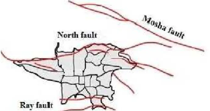
One of the top ten ranks in the context of earthquake vulnerability is Iran country which has earthquake vulnerability with intensity greater than 5.5 on the Richter scale (Mohamadi et al., 2015). Meanwhile, the Iranian capital that is Mega City of Tehran with a population of 9476821 people is strongly under vulnerability condition. With respect to the fact that there exist many of faults and historical records of faults activity which it can be understood that in the approach time, earthquake vulnerability will leave many damages and loss in stock. In this paper, a case study in region 20 of Tehran is implemented. This region is the southern point of Tehran city which has 20 sectors. Its area is 176 km2, and its population is 340247 people based on the census of 2011. Old neighborhoods are one of the outstanding features of the region. This region is one of the oldest urban regions of Iran. The district is threatened by Ray Fault and other faults under Tehran city and positioned in Sorkh-e-Hesar downstream (See Figure 1).

Figure 1. Map of Tehran faults and Ray fault lying on region 20 of Tehran

The map of this region with detail is shown in Figure 2. In 2012, a comprehensive paper was presented on this region using probabilistic risk analysis. One of the important systematic approaches is probabilistic risk analysis which capable of providing both fields of sciences and multiple expertizes in order to a comprehensive analysis of performance of engineering systems. In addition, an efficient managerial tool for disaster managers is risk analysis which can help in decision making using various methods to explore reactions to vulnerabilities and probable risks. Norouzi Khatiri et al. (2013) calculated vulnerability of buildings considering earthquake disaster using this tool (See Figure 3) which this paper, has manly used to validate the case study and exact programming on the region. In this case study has been considered three scenarios with probabilities of 0.4, 0.35, and 0.25 with regard to the subject matter experts on the basis of historical records.

43

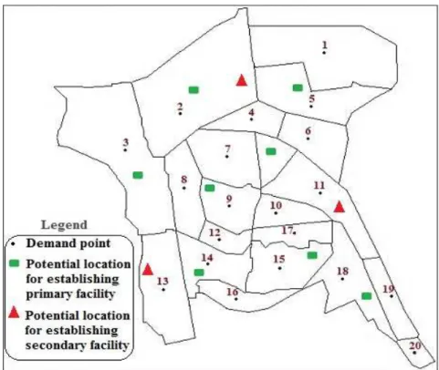
Figure 2. Region 20 of Tehran map containing the potential locations of primary

and secondary facility and demand point

44

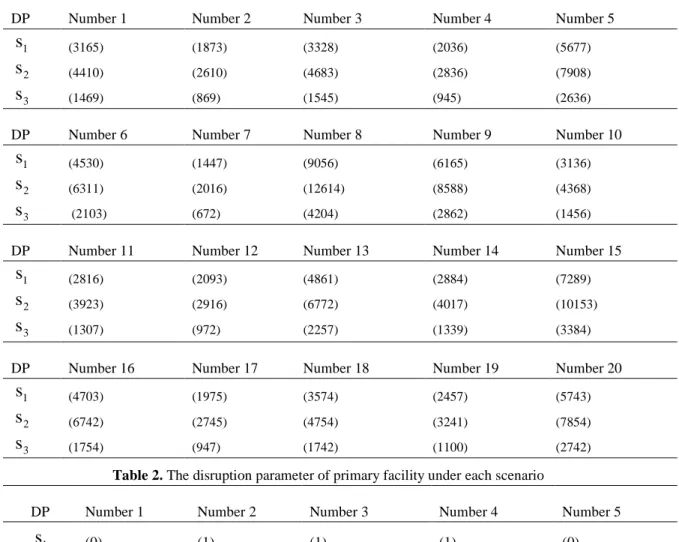
Due to the existence of 20 sectors in region, 20 demand points and 10 potential locations for establishing primary facilities have been considered, in addition, 3 potential locations are regarded for establishing the secondary facilities. These points and their coordinates have been illustrated in Fig. 2. The capacity of the primary and secondary facilities is set to be 40000 and 60000 respectively. The distance of each route has been calculated by using Tehran navigation website (http://map.tehran.ir/) With regard to region's area, the maximum number of primary and secondary facilities which should be established is 5 and 2 respectively. The demand for relief commodity at each demand point for a given scenario is presented as shown in Table 1. With regard to the vulnerability probability and other considerations, the disruption of each primary facility has been calculated in Table 2.

Table 1. The stochastic demands for relief commodities under each scenario

Number 5 Number 4 Number 3 Number 2 Number 1 DP (5677) (7908) (2636) (2036) (2836) (945) (3328) (4683) (1545) (1873) (2610) (869) (3165) (4410) (1469)

Number 10 Number 9 Number 8 Number 7 Number 6 DP (3136) (4368) (1456) (6165) (8588) (2862) (9056) (12614) (4204) (1447) (2016) (672) (4530) (6311) (2103)

Number 15 Number 14 Number 13 Number 12 Number 11 DP

(7289) (10153) (3384) (2884) (4017) (1339) (4861) (6772) (2257) (2093) (2916) (972) (2816) (3923) (1307)

Number 20 Number 19 Number 18 Number 17 Number 16 DP

(5743) (7854) (2742) (2457) (3241) (1100) (3574) (4754) (1742) (1975) (2745) (947) (4703) (6742) (1754)

Table 2. The disruption parameter of primary facility under each scenario

Number 5 Number 4 Number 3 Number 2 Number 1 DP (0) (1) (1) (1) (1) (0) (1) (1) (0) (1) (0) (1) (0) (1) (1) Number 8 Number 7 Number 6 DP (1) (1) (0) (0) (0) (1) (1) (1) (1) 1

s

2

s

3

s

1

s

2

s

3

s

1

s

2

s

3

s

1

s

2

s

3

s

1

s

2

s

3

s

1

s

2

s

3

s

45

7- Findings and results

In this section, the problem has been solved considering case study data and results have been presented. The problem has been solved by CPLEX and all tests are implemented on personal computer with processor Core (TM) i3, 2.27 HZ.

As mentioned before, we used Ɛ_{-constraint to solve model. First, for obtaining}

2

ε

, the model was solved without notice to objective function Z1and

ε

2 considered equal to achieved quantity of objective function and then we transforming with Z₂ to constraints. Then we analyze behavior of model by changing the quantity of

ε

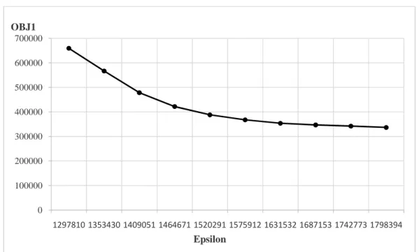
₂. The results are presented in Tables 3.

As we expected, the value of objective function 1 decreases when

ε

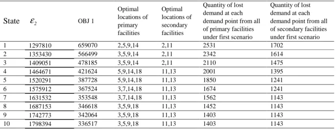
₂ increases due to improving the solution space, therefore, decision makers can choose the best path with considering the balance between objective function 1 and objective function 2.

Table 3. The results of using different

ε

₂

Quantity of lost demand at each demand point from all of secondary facilities under first scenario Quantity of lost

demand at each demand point from all of primary facilities under first scenario Optimal locations of secondary facilities Optimal locations of primary facilities OBJ 1 2

ε

State 1702 2531 2,11 2,5,9,14 659070 1297810 1 1614 2342 2,11 3,5,9,14 566499 1353430 2 1475 2110 2,11 3,5,9,14 478185 1409051 3 1395 2001 11,13 5,9,14,18 421624 1464671 4 1241 1850 11,13 5,9,14,18 387728 1520291 5 1241 1674 11,13 3,7,14,18 367524 1575912 6 1143 1562 11,13 3,7,14,18 353548 1631532 7 1143 1452 11,13 3,5,9,18 346618 1687153 8 1143 1403 11,13 3,5,9,18 342064 1742773 9 1143 1403 11,13 3,5,9,18 336517 1798394 10

Variation of first objective function with different value of

ε

2is shown more clearly in Figure 4.

As can be seen in the Figure 4, if the value of

ε

₂increases to 1520291, then the variation of the first objective function remains steady. Therefore, it is better for decision maker to select the case of 150291 or higher.

As a result of increasing value of

ε

2, decreasing lost demand and consequently improving first objective function are observed as shown in Fig. 5.

7-1- Validation of the model

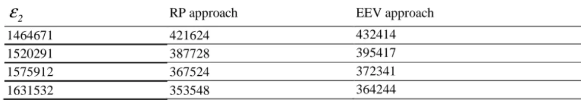
After obtaining quantities of decision variables, we use some factors to demonstrate the usefulness of the model, these factors are:

1. EEV approach: Value of the expected value solution 2. RP approach: Value of the expected value solution

46

Figure. 4. Variation of first objective function depending on different value of

ε

₂

.

Figure 5. Variation of lost demand depending on different value of

ε

₂

.

An interesting vision can be obtained from Table 4, where a comparison of two measures is presented for the cases of 4, 5, 6, and 7.

0 100000 200000 300000 400000 500000 600000 700000

1297810 1353430 1409051 1464671 1520291 1575912 1631532 1687153 1742773 1798394

Epsilon OBJ1

0 500 1000 1500 2000 2500 3000

1297810 1353430 1409051 1464671 1520291 1575912 1631532 1687153 1742773 1798394

47

Table 4. Comparison of the results

2

ε

RP approach EEV approach

1464671 421624 432414

1520291 387728 395417

1575912 367524 372341

1631532 353548 364244

As seen in Table 4, with respect to the more awareness on the conditions, in RP approach, objective function of RP approach is better than EEV. This report confirms the accurateness of two-stages stochastic program and give the consistent results for the presented model.

8- Conclusion

In this paper, we developed a mixed nonlinear integer bi-objective model for the stochastic RLRP where substantial improvements in reliability can be attained with considering primary and secondary depot. Our model formulation was a two stage stochastic approach that, in first stage, strategic location decisions should be made before any failure occurs and in two stages routing decisions are made in the future after the uncertainty has been resolved. The model included two objectives. The first objective function minimized the sum of the fixed primary and second facilities-establishing cost, and the sum of the expected dispatching cost for the vehicles assigned and shortage cost, respectively. Also, the second objective function minimized expected value of total impedance value-weighted travel distance. The ε

-constraint has been adapted for solving the proposed model, we analyzed our model by using different values of ε_{-constraint, and decision maker could select the best approach by attention to this analysis. The}

result shown that with respect to the more awareness on the conditions, in RP approach, objective function of RP approach is better than EEV.

There exist some topic for more research in this topic which is proposed:

1. Using robustness criteria such as minimax cost, minimax regret and p-robustness for providing decision support.

2. It can be possible to consider location–routing together with other supply chain problems, such as inventory management.

3. Designing of metaheuristic algorithm for large scale problem for this model. 4. Using Compromise Programming or other method to solve the bi-objective model.

48 References

Aboolian, R., Cui, T., & Shen, Z. J. M. (2012). An efficient approach for solving reliable facility location models. INFORMS Journal on Computing,25(4), 720-729.

Ahmadi-Javid, A., & Seddighi, A. H. (2013). A location-routing problem with disruption risk. Transportation Research Part E: Logistics and Transportation Review, 53, 63-82.

Albareda-Sambola, M., Fernández, E., & Laporte, G. (2007). Heuristic and lower bound for a stochastic location-routing problem. European Journal of Operational Research, 179(3), 940-955.

Avriel, M. (1980). A geometric programming approach to the solution of location problems. Journal of

Regional Science, 20(2), 239-246.

Chen, Q., Li, X., & Ouyang, Y. (2011). Joint inventory-location problem under the risk of probabilistic facility disruptions. Transportation Research Part B: Methodological, 45(7), 991-1003.

Cui, T., Ouyang, Y., & Shen, Z. J. M. (2010). Reliable facility location design under the risk of disruptions. Operations Research, 58(4-part-1), 998-1011.

Etemadnia, H., Goetz, S. J., Canning, P., & Tavallali, M. S. (2015). Optimal wholesale facilities location within the fruit and vegetables supply chain with bimodal transportation options: An LP-MIP heuristic approach. European Journal of Operational Research, 244(2), 648-661.

Haimes, Y. Y., Ladson, L. S., & Wismer, D. A. (1971). Bicriterion formulation of problems of integrated system identification and system optimization. IEEE Transactions on Systems Man and Cybernetics, (3), 296.

Hassan-Pour, H. A., Mosadegh-Khah, M., & Tavakkoli-Moghaddam, R. (2009). Solving a multi-objective multi-depot stochastic location-routing problem by a hybrid simulated annealing algorithm. Proceedings of the Institution of Mechanical Engineers, Part B: Journal of Engineering

Manufacture, 223(8), 1045-1054.

Herazo-Padilla, N., Montoya-Torres, J. R., Munoz-Villamizar, A., Nieto Isaza, S., & Ramirez Polo, L. (2013, December). Coupling ant colony optimization and discrete-event simulation to solve a stochastic location-routing problem. In Simulation Conference (WSC), 2013 Winter (pp. 3352-3362). IEEE.

Horner, M. W., & O'Kelly, M. E. (2001). Embedding economies of scale concepts for hub network design. Journal of Transport Geography, 9(4), 255-265.

http://map.tehran.ir/

Javid, A. A., & Azad, N. (2010). Incorporating location, routing and inventory decisions in supply chain network design. Transportation Research Part E: Logistics and Transportation Review, 46(5), 582-597. Klibi, W., Lasalle, F., Martel, A., & Ichoua, S. (2010). The stochastic multiperiod location transportation problem. Transportation Science, 44(2), 221-237.

Mohamadi, A., Yaghoubi, S., & Derikvand, H. (2015). A credibility-based chance-constrained transfer point location model for the relief logistics design (Case Study: earthquake disaster on region 1 of Tehran city).International Journal of Supply and Operations Management, 1(4), 466-488.

49

Norouzi, K. K., Omidvar, B., Malek, M. B., & Ganjehi, S. (2013). Multi-Hazards risk analysis of damage in urban residential areas (Case study: earthquake and flood hazards in tehran-iran). Journal of

Geography and Environmental Hazards, 2(7), 566-608.

Peng, P., Snyder, L. V., Lim, A., & Liu, Z. (2011). Reliable logistics networks design with facility disruptions. Transportation Research Part B: Methodological, 45(8), 1190-1211.

Snyder, L. V. (2003). Supply chain robustness and reliability: Models and algorithms (Doctoral dissertation, Northwestern University).

Snyder, L.V., Daskin, M.S., (2005). Reliability models for facility location: the expected failure cost case. Transp. Sci. 39 (3), 400–416

Wei-long, Y. E., & Qing, L. I. (2007, August). Solving the Stochastic Location-Routing Problem with Genetic Algorithm. In Management Science and Engineering, 2007. ICMSE 2007. International

Conference on (pp. 429-434). IEEE.

Xie, W., Ouyang, Y., & Wong, S. C. (2015). Reliable Location-Routing Design Under Probabilistic Facility Disruptions. Transportation Science.

Yeager, C. D., & Gatrell, J. D. (2014). Rural food accessibility: An analysis of travel impedance and the risk of potential grocery closures. Applied Geography, 53, 1-10.

Zhang, B., Ma, Z., & Jiang, S. (2008, October). Location-routing-inventory problem with stochastic demand in logistics distribution systems. In Wireless Communications, Networking and Mobile

Computing, 2008. WiCOM'08. 4th International Conference on (pp. 1-4). IEEE.

Zhang, Y., Qi, M., Lin, W. H., & Miao, L. (2015). A metaheuristic approach to the reliable location routing problem under disruptions. Transportation Research Part E: Logistics and Transportation