An approximation algorithm and FPTAS for Tardy/Lost minimization with common due dates on a single machine

An approximation algorithm and FPTAS for Tardy/Lost

minimization with common due dates on a single machine

Kamran Kianfar

, Ghasem Moslehi

*, Ali Shahandeh Nookabadi

Faculty of Engineering, University of Isfahan, Isfahan, Iran 2

Department of Industrial and Systems Engineering, Isfahan University of Technology, Isfahan, Iran

[email protected], [email protected], [email protected]

Abstract

This paper addresses the Tardy/Lost penalty minimization with common due dates on a single machine. According to this performance measure, if the tardiness of a job exceeds a predefined value, the job will be lost and penalized by a fixed value. Initially, we present a 2-approximation algorithm and examine its worst case ratio bound. Then, a pseudo-polynomial dynamic programming algorithm is developed. We show how to transform the dynamic programming algorithm to an FPTAS using the technique of "structuring the execution of an algorithm" and examine the time complexity of our FPTAS.

Keywords:Single machine scheduling, Tardy/Lost penalty, Common due date, approximation algorithm, FPTAS

1- Introduction

In this paper, we study a single machine scheduling problem related to minimizing total Tardy/Lost

penalties and common due dates. Every job 1 ≤ ≤ has a processing time, , and a weight

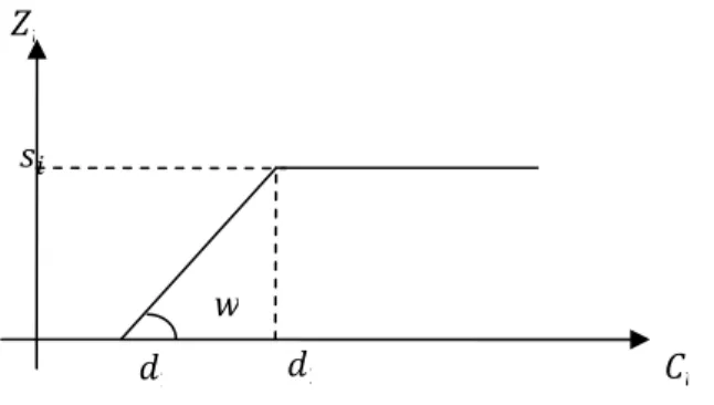
tardiness factor, . The jobs have two common due dates, namely, and . In case a job is

completed before the first due date, , no penalty is assigned; if the completion time is between

and , the job will be penalized by a linear tardiness penalty; and finally, the job will be lost and a

fixed amount of penalty, , will be assigned if it is completed after the second due date, . Based on

this formulation, we can define the Tardy/Lost objective function as shown in Eq. (1), where is the completion time of job i in a sequence.

= ₌ 0, −_{− >} ≤ 1

Figure 1 shows the Tardy/Lost penalty function for job i based on its completion time.

*Corresponding author.

ISSN: 1735-8272, Copyright c 2016 JISE. All rights reserved

Journal of Industrial and Systems Engineering Vol. 9, No. 2, pp 1-19

Fig. 1. Tardy/Lost penalty function with common due dates

We assume that all processing times and due dates are integers, the machine is continually available from time zero and it can process at most one job at a time. The resulting problem is denoted by 1| = | , where TL indicates the Tardy/Lost performance criteria. Yuan (1992) has shown that the tardiness minimization problem with a common due date (CD_T) is NP-hard. Since CD_T is a special case of Tardy/Lost penalty function evaluated in this paper, this function is also assumed to be NP-hard.

Objective functions of real-life manufacturing problems are often much more complex than the well-known scheduling performance measures. Depending on the type of contractual penalties and the expected goodwill of future revenue losses incurred, many types of non-linear tardiness penalty functions may arise. Tardy/Lost measure combines the futures of two objective functions: weighted tardiness and weighted number of tardy jobs.

From a practical point of view, the TL penalty function is applicable in delivery contracts, most of which are arranged based on two due dates. If an order is early, then no penalty is considered; the order will be penalized if its delivery time exceeds the first due date. The penalty is increased in proportion to the delivery time until the second due date is reached. If the delivery occurs later than the second due date, the order becomes lost and gets the maximum fixed penalty.

The Tardy/Lost performance measure can be considered as a special case for scheduling problems with order acceptance assumption. Here, the objective is minimizing weighted tardiness on a single

machine and a common due date where the rejection cost for a job i can be defined as − .

Order acceptance assumption has been investigated widely in the literature. Engels et al. (2003) investigated the problem of minimizing weighted completion times and rejection penalties and developed some approximation algorithms. The survey papers by Slotnick (2011) and Shabtay (2013) have addressed a number of scheduling problems with order acceptance.

The performance measure we consider in this study is a kind of regular measure which is continuous and non-decreasing in the completion times of jobs. With such performance measures, jobs are penalized only for being tardy, while all inventory costs due to early completions are ignored. Pinedo(1995) indicates that in practice, the penalty function associated with a scheduling problem may follow from a function in which early jobs are assigned no penalty and those finished after their due dates are assigned a penalty that is increased at a given rate. Within the penalty function, the job reaches a point where the penalty assignment is changed and increased at a much slower pace. The function identified by Pinedo(1995) is general; however, two more specific functions that react similarly are the deferral cost function (Lawler, 1964) and the late work criterion (Potts and Vav Wassenhove, 1992a, Potts and Vav Wassenhove, 1992b).

Assume that we have an approximation algorithm that always returns near-optimal solution whose

cost is at most a factor of ! away from the optimal cost, where ! > 1 is a real number. In

minimization problems the near-optimal cost is at most a multiplicative factor of ! above the

optimum. Such an approximation algorithm is called a !-approximation algorithm. A family of (1+"

approximation scheme, or PTAS for short. If the time complexity of a PTAS is also polynomially

bounded in 1/", then it is called a fully polynomial time approximation scheme, or FPTAS for short

(Woeginger, 2000).

Deferral cost functions have been studied by Kahlbacher(1993). He considered general penalty functions to be monotonous with respect to absolute lateness. He also examined several specific cases of the penalty function for situations in which machine idle times are allowed (the unconstrained problem) or not allowed (the constrained problem). Using the "V-shape property", he constructed an optimal schedule with a pseudo-polynomial algorithm and extended it to an FPTAS of the order$ %⁄" , where " denotes the precision of the approximation solution.

Federgruen and Mosheiov (1994) considered a class of single machine scheduling problems with a common due date and general earliness and tardiness penalties. In that study, some polynomial greedy algorithms were proposed for generating schedules and a small optimality gap was illustrated through numerical examples. For convex cost structures, they also established that the worst case optimality gap was bounded by 0.36 if the due date was non-restrictive. Baptiste and Sadykov (2009) considered the objective of minimizing a piecewise linear function. This class of functions is very large and can also be used to model some classical objective functions, i.e., total (weighted) completion time, total (weighted) tardiness, and (weighted) number of tardy jobs. They introduced a new Mixed Integer Programming (MIP) model based on time interval decomposition. This MIP model was closely related to the classical time-indexed MIP formulation, but used far fewer variables and constraints.

The research by Ventura and Radhakrishnan (2003) focused on scheduling jobs with varying processing times and distinct due dates on a single machine. Zhou and Cai (1997) examined two types of regular performance measures, the total cost and the maximum cost, with general cost functions. They studied a stochastic scheduling model on a single machine where processing times were random variables and the machine was subject to stochastic breakdowns. In the paper by Shabtay (2008), two continuous and non-decreasing objective functions were considered. They included penalties due to earliness, tardiness, the number of tardy jobs, and due date assignments.

In the present study, we simply observe that the Tardy/Lost penalty function can be converted to a late work criterion that estimates the quality of a solution on the basis of the duration of the late parts

of jobs. This conversion is accomplished by setting = 1 ∀ = 1, . . . , and = + , where

and are the first and second due dates for each job i. The results concerning late work

scheduling problems are partially presented in Chen et al. (1998) and Leung (2004), but Sterna (2011) offers the first complete review of the topic.

A number of researchers have addressed the problem of minimizing the total late work criterion on a single machine. Potts and Van Wassenhove (1992b) proposed a polynomial time algorithm based on the similarity between tardiness and late work parameters. In another study (Potts and Vav Wassenhove, 1992a), they developed a branch-and-bound algorithm for a problem forming the core of a family of approximation algorithms based on truncated enumeration. References (Sterna, 2007b, Pesch and Sterna, 2009, Sterna, 2007a, Blazewicz et al., 2008, Ren et al., 2009) may be consulted for other studies devoted to the late work criterion.

Kathley and Alidaee (2002) modified the definition of the late work criterion by introducing two due dates for each job, called due date and deadline. They called the proposed performance criterion "modified TWLW", which was very similar to the Tardy/Lost penalty function we have considered in this study. Kianfar and Moslehi (2013, 2014)studied some tardiness-based objective functions on a single machine with common due dates. They developed approximation algorithms as well as FPTASs for the problems. The worst-case ratio bounds are also proved in some cases.

As the Tardy/Lost penalty function is a general form of the late work criterion, most practical applications of late work can be equally defined by this penalty function. Some of the applications in problems arise in control systems (Blazewicz, 1984, Potts and Vav Wassenhove, 1992b), production and planning process (Sterna, 2000, sterna, 2006), agriculture (Alminana et al., 2010), land cultivation processes (Blazewicz et al., 2004, Sterna, 2000), and processes of planning tests for prototypes or software validation (sterna, 2006).

The rest of this paper is organized as follows. In Section 2, we propose an approximation algorithm and examine its worst case ratio bound. Section 3 describes a pseudo-polynomial dynamic

programming algorithm that, in Section 4, will be converted to an FPTAS using the technique of structuring the execution of an algorithm. Concluding remarks will be presented in Section 5.

2- MWR

approximation algorithm

Here, a 2-approxiamtion algorithm is developed for problem 1| = | . By using a numerical

example in a later stage, it will be shown that the worst case ratio bound of 2 is tight for this problem. We refer to this algorithm as MWR and designate the sequence it generates as G. We adopt the notation *_{[ ]}to represent the job in ith position in the sequence- = *_{[ ]}, *_{[ ]}, . . . , *_[.] . Heuristic G

requires at most n iterations, while, in each iteration k, the (n-k+1)th element of G, *_{[./01 ]} will be

determined. Furthermore, if, during an iteration, there exists an unscheduled job filling the remaining

tardiness period with the minimum tardiness weight, the relevant sequence (sequence -2) will be saved

in addition to the main sequence G. The algorithm returns the best of the two sequences G and -2 as

the final result.

Let 3denote the penalty of sequence G and _4[5,6]denote the total penalty of jobs from position

rton in this sequence. Suppose that all jobs iare sorted and indexed according to the non-decreasing

order of ⁄ ratios. In the case of a tie, the job with the smallest processing time should come first.

The steps of the algorithm are as follows:

Step 1.Let 7 = 1,2, . . , be a set of unscheduled jobs sorted according to their indices

(according to the non-decreasing order of ⁄ ratios). Set _[.] = 9_:;<= ∑._> and ? = .

Step 2.Define 7@ = A ∈ 7 | ≥ _[.]− D. If 7@ is empty, then E_FG:H= ∞; else, select a job

Ĵwith the minimum tardiness weight from 7@. Let *L_[.]= Ĵand E_FG:H= _M̂N A _[.], D − O.

Step 3.Define the first job in U as job k; also, set 7 = 7/ P , *_[Q]= Pand _{[Q/ ]}= _[Q]− ₀.

Step 4.If 7@ = A ∈ 7 | ≥ _{[Q/ ]}− D is not empty, select a job Ĵ with the minimum tardiness

weight from 7@. Calculate E = _M̂N A _{[Q/ ]}, D − O. If E + _4[Q,.]< E_FG:H then we have

E_{FG:H = E + 4[Q,.]} and *L_{[ ]}= *_{[ ]} ∀ = ?, . . . , and *L_{[Q/ ]}= Ĵ.

Step 5.If _{[Q/ ]}> , then ? = ? − 1 and go back to Step 3; else, go to Step 6.

Step 6.Put unscheduled jobs at the beginning of each of the sequences Gand -2.

Step 7.If 3≤ 32, then return sequence - = N*_{[ ]}, *_{[ ]}, . . . , *_[.]O; else, return sequence -2 =

N*L[ ], *L[ ], . . . , *L[.]O.

It can be easily verified that G has the same order as WSPT and -2is the best sequence obtained by

filling the remaining tardiness period with one job in each iteration. This algorithm includes a simple

sorting of n elements and hence, its time complexity is$ ST* .

Now, we provide a numerical example to illustrate how the MWR algorithm works. Later, we will use a theorem to prove that the worst case ratio bound of this algorithm is equal to 2.

Example 1.Consider a problem 1| = | with 4 jobs described in Table 1. Set = 10and

= 12.

1_{- Minimum Weight Ratio}

Table 1.Parameters of jobs in Example 1

Job i

2 5

1

3 4

2

5 6

3

16 15

4

At the beginning, 7@ is empty and E_FG:H = ∞. The following table summarizes the results of

algorithm MWR for this problem.

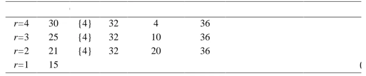
Table 2.Summary of applying MWR algorithm for Example 1

U

36 4

32 {4} 30

r=4

36 10

32 {4} 25

r=3

36 20

32 {4} 21

r=2

15

r=1

From 3 = 52and 32= E_FG:H= 36, algorithm MWR returns sequence -2 as the approximate

solution.

Theorem 1.Algorithm MWR gives a 2-approximation for problem1| = | .

Proof. See the Appendix. ■

In the following example, we show that the worst case ratio bound of algorithm MWR for problem

1| = | is a tight bound.

Example 2.Consider the problem 1| = | with > 2jobs such that = − 1and =

2 − 1. The parameters are those given in Table 3.

Table 3.Parameters of jobs in Example 2

Job i

n+1/n n

1

1+1/n 1

2 to n

Algorithm MWR returns the sequence 2,3, . . . , , 1 with a penalty value of + 1while the

optimal sequence is 1,2, . . . , , generating the penalty 1 2⁄ + 2 − 1 2⁄ . Thus,

3

∗ = _{+ 2 −}+ 1 ⇒ S_.→\ 3

∗ = 2 2

3- Dynamic programming algorithm

Suppose that jobs are indexed according to the non-decreasing order of ⁄ and ties are broken by

first selecting a job with the minimum . An optimal solution is composed of three groups of jobs.

The first group includes early jobs with completion times less than . The second group includes the

tardy jobs with completion times between and , which must be scheduled according to their

reverse order of indices (the first tardy job, called straddling job, may not adopt this order). Lost jobs

The problem can be optimally solved by applying the following dynamic programming algorithm. In this algorithm, each state in the state space ]₀^,_` shows a particular sequence for first k jobs

excluding the straddling one, where the straddling job a and its completion time, _^, are predefined.

We use the vector b , b , to denote states. Variables b and b show the sum of processing times

for jobs in the first and second groups, respectively, and f is the total penalty of the corresponding partial sequence.

In each iteration, the algorithm selects a job a as the straddling and fixes its completion time, _^,

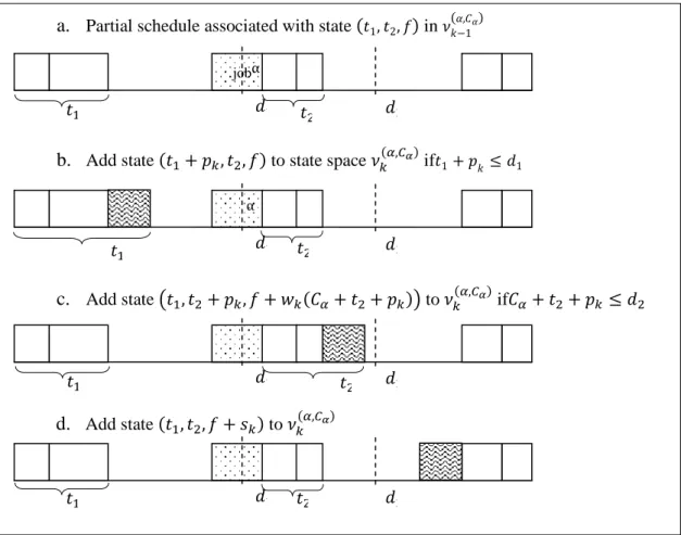
from all possible values within the scheduling horizon. Jobs in the first group, early jobs, are continually scheduled from time zero (see Fig. 2b) while tardy jobs are scheduled by starting from the completion time of the straddling job (see Fig. 2c). Finally, lost jobs are scheduled in such a way that they are completed at time 9_:;<= ∑._> (see Fig. 2d).

Let _{^,_}∗ _` denote the optimal objective value subject to the condition in which job a is selected as

the straddling one with the completion time _^. This algorithm can be described as follows.

Algorithm DP

1.1. Set ]_c^,_` = 0,0,0

1.2. For each P = 1,2, . . . , a − 1, a + 1 , . . . , , consider all the states b , b , in ]_0/^,_`

o If b + ₀ ≤ _^− _^, then add the state b + ₀, b , to the state space ]₀^,_`

o If _^+ b + ₀ ≤ , then add the state Nb , b + ₀, + _{0 ^}+ b + ₀− O to the state space ]₀^,_`

o Add b , b , + ₀ to the state space ]₀^,_`

1.3. For all states b , b , ∈ ]₀^,_` with equal values for b and b , keep at most one state having the minimum value of f.

1.4. Remove the state space ]_0/^,_`

1.5. Set _{^,_}∗ _`=

[Hd,He,f]∈g6hd`,i`

+ ^. ^, −

Step 2. Return the optimal solution ∗=

^,_` ^,_`

Fig. 2 Description of the dynamic programming algorithm

To calculate the time complexity of this algorithm, as all input parameters are integers, we can

restrict the number of states in each ]₀^,_` by − . This is because variables b and b can at

most take and − different values, respectively. Also, in each iteration and for each

combination of b and b , we keep at most one state with the smallest value of f.

Let 9_<jk be the maximum processing time of jobs. The running time of Step 1.2.is proportional to

∑./ l]₀^,_` _l

0> and hence, it is − . Similarly, it can be shown that the complexity of step

1.5 is $N − O. Step 1 iterates at most 9_<jktimes by selecting different a and _^ values and

has the complexity of $N 9_<jk − O. Finally, as Step 2 needs $ 9_<jk time, the total

complexity of this algorithm will be obtained as $N 9_<jk − O. Alternatively, we can write

the complexity of this algorithm as $N 9_:;< − O because the maximum number of

iterations created by selecting the values of α and _^ can also be considered as 9_:;<instead of 9_<jk.

4- FPTAS algorithm

This FPTAS is based on two phases. In the first phase, algorithm MWR is used to determine an

upper bound for problem 1| = | and in the second phase, the execution of the algorithm DP is

modified in order to reduce the number of states and the running time. One common way used for transforming a dynamic programming algorithm to FPTAS is the technique of structuring the

execution of an algorithm. The main idea of this technique is to remove a special part of states

generated by the algorithm in such a way that the modified algorithm becomes faster, yielding an approximate solution instead of the optimal one. This method was first introduced by Ibarra and Kim

b

a. Partial schedule associated with state b₁, b₂, in ]_P−1a, a jobα

b. Add state b + ₀, b , to state space ]₀^,_` ifb₁+ _P≤ ₁

c. Add state Nb , b + ₀, + _{0 ^}+ b + ₀ O to ]₀^,_` if _^+ b + ₀ ≤

d. Add state b , b , + ₀ to ]₀^,_`

b

α b

b

b

b b

(1875) for solving the knapsack problem and it has been extended to numerous scheduling problems (see (Shabtay et al., 2012, Shabtay and bensoussan, 2010, Ji and Cheng, 2010, Steiner and Zhang, 2009, Kacem and Mahjoub, 2009)).

Let _n denote the objective value returned by algorithm MWR for an instance of the problem

1| = | and ε be the maximum acceptable error for the FPTAS. According to the technique of structuring the execution of an algorithm, we should restrict all factors that allow the size of the state

space to grow in an uncontrolled way. These factors in our algorithm are the variables b and fin the

states b , b , as well as the completion time of the straddling job.

By selecting a job a as the straddling, we split its completion time interval _^∈ [ + 1 , + _^]

into sub-intervals qr ₁+ s_{1 t−1}u,v ₁+ s_{1 t}wx, where s = 1 + " 3⁄ and t = 1,2, . . . , . The maximum number of these sub-intervals is

= yST*_z{_d`_{| ≤ yST*}

zd

}~•€_{| = •S 9}

<jk⁄S s ‚ ≤ • 1 + 3 "⁄ S 9<jk‚ 3

So, we have = $ S 9_<jk⁄" . The last inequality holds since for all ƒ ≥ 1, we have S ƒ ≥

ƒ − 1 ƒ⁄ based on the Taylor expansion of ln z. Therefore,

1

S s ≤s − 1 =s 1 + " 3 − 11 + " 3⁄⁄ = 1 + 3 "⁄ 4

To restrict the number of different values for b , set … = _n⁄2 and s = ". … 3⁄ . Let there

be m distinct values among tardiness weights of n jobs. Sort these values in a decreasing order

such that _†d> _†e> . . . > _†~and create the permutation ‡ = ˆ , ˆ , . . . , ˆ_< . Split the interval

q0, n⁄ †~x into m intervals

‰ = Š0, n

†d‹ , ‰ = Š

n †d,

n

†e‹ , . .. , ‰<= Š

n †~hd,

n

†~‹ 5

Then, split each interval ‰_Œ into the sub-intervals of the length s Ž . _†• . It may appear that the

last of the sub-intervals of an interval ‰_Œ is shorter than s Ž . _†• . The maximum number of

sub-intervals created by the above procedure is

= n

†d×

. †d

s + • Š n†‘−

n †‘hd‹

< >

. †‘

s ≤ . • ’ n

†‘ .

†‘

s “ ≤ . .s ≤n

< >

._sn

6

and since _n⁄ = 2 … ss ⁄ ≤ 6 "⁄ , we conclude that = $ %⁄" .

In order to make the number of distinct values of f controllable, we split the related interval [0, _n]

into _% equal sub-intervals ‰′_< = [ − 1 s_%, s_%] of the length s_% ,where1 ≤ ≤ _%.

Considering _%= •2 "⁄ ‚and s_%= _n⁄ _%, we get _%= $ ⁄" .

Next, the FPTAS algorithm will be designed by means of bounding the number of different values that each of variables _^, b and fcan take in the DP algorithm. Also, the time complexity of this FPTAS as well as its worst case ratio bound will be discussed.

This FPTAS works on a reduced state space ]₀^,_•`# instead of the main state space ]<sub>0</sub>^,_` and

Algorithm FPTAS

Step 1. For each a = 1,2, . . . , and each ′_^= — + s ˜™ , t = 0,1, . . . ,

1.1. Set ]_c^,_•`#= 0,0,0

1.2. For each P = 1,2, . . . , a − 1, a + 1 , . . . , , consider all the states b , b , in ν_›/œ,••ž #

o If b + ₀ ≤ _^− _^, then add state b + ₀, b , to the state space ]₀^,_•`#

o Add Nb , b + ₀, + _{0 ^}+ b + ₀, − O to the state space ]₀^,_•`#

o Add b , b , + ₀ to the state space ]₀^,_•`#

1.3. For all states b , b , ∈ ]₀^,_•` # with equal values for b and b , keep at most one state with the minimum value of f.

1.4. Remove the state space ]_0/^,_•` #

1.5. Keep at most one state with the smallest value of b among all states b , b , ∈ ]₀^,_•`#

laying in common sub-intervals for b and f .

1.6. Set _{^,_•}# _`=

[Hd,He,f]∈g6hd`,iŸ` #

+ ^. ′^, −

Step 2. Return the approximate solution #=

^,_•` ^,_•`

#

In the FPTAS algorithm, we have replaced the statement “if _^+ b + ₀ ≤ , then add state

Nb , b + 0, + 0 ^+ b + 0− O” from step 1.2 of the DP algorithm with phrase “add state

Nb , b + 0, + 0 ^+ b + 0, − O”. Here, we have two cases:

^+ b + 0 ≤ ⇒ 0 ^+ b + 0, − = 0 ^+ b + 0−

^+ b + 0 > ⇒ 0 ^+ b + 0, − = 0 − = 0

The first case shows the same condition as in the DP algorithm and in the second case, job k is

scheduled in the second group, but its completion time is greater than and its tardiness penalty

equals ₀. According to this, we do not need to restrict variable b in the FPTAS because penalties are

calculated correctly and from Eqs (5) and (6), the number of intervals for variable b is $ %⁄" , which is sufficient for the FPTAS.

4-1- Analysis of worst case ratio bound

The worst case analysis of this FPTAS will be based on comparing the steps of algorithms DP and FPTAS. We may remark that the main action of FPTAS consists of reducing the cardinality of the

state spaces by splitting the intervals of _^, b and finto sub-intervals and then replacing all vectors

b , b , ∈ ]₀^,_` # _{belonging to the same sub-intervals by a single approximate state with the}

smallest b . Let _<jk0 denote the maximum tardiness weight for a tardy job in the DP between jobs

kton.

<jk0 = 01 | 0 ≤ ≤ − P , 01 > ^ 7

Lemma 1.Suppose b , b , is an arbitrary state in ]₀^,_` . Algorithm FPTAS creates at least one state Nb#, b#, #O in ]<sub>0</sub>^,_•` # such that

b# _{≤ b 8}

b# _{≤ b + P. s N .} <jk0 O

⁄ 9

# _{≤ + Ps + Ps}

%+ " 3⁄ 10

Proof. The proof is done by induction on parameter k. First, for P = 0, the statement is trivial because]_c^,_•`# = ]<sub>c</sub>^,_` . Now, assume that the lemma holds up to level k-1and we want to show that it is valid for level k. Consider an arbitrary state b , b , ∈ ]₀^,_` . Algorithm DP introduces

this state into ]₀^,_` when job k is added to some feasible state for the first k-1 jobs. Let b′ , b′ , ′

be the above feasible state.

If _<jk0 = 0, the proof is trivial because in this case, there is no tardy job in the DP between jobs k and n and the DP algorithm schedules the remaining jobs as early. In this condition, the FPTAS

algorithm can also schedule the remaining jobs as early, because b# ≤ b and there is enough empty

space for the early jobs in the FPTAS. In other words, _<jk0 = 0 means that the penalty for the DP

remains unchanged from steps k to n and the FPTAS algorithm is also able to create a state in the final step n with the same penalty as state k. So, the proof of lemma 1 is obvious in this condition.

According to the above discussion, we assume _<jk0 > 0 in the rest of the proof.

Let _^ and ′_^ denote the completion time of the straddling job in algorithms DP and FPTAS,

respectively. Also, let _^∗ and ′_^ be the tardiness of the straddling job in these two algorithms. The

FPTAS algorithm considers the completion time for the straddling job as ′_^= — + s ˜™ , t =

0,1, . . . , . This divides the possible interval [ + 1, + _^] into integer subintervals [• +

s ˜/ _{‚, — + s} ˜_{™] , t = 1, . . . , . Given the fact that the completion time of the straddling}

job in the DP, _^, also falls in interval [ + 1, + _^], we have

∀ Cœ∈ I¦= [•d + Δ ¦/ ‚, —d + Δ ¦™] ⇒ ∃C′œ= —d + Δ ¦™ ∀y = 1, . . . , L

⇒ Cœ≥ d + Δ ¦/ ⇒ Cœ− d ≥ Δ ¦/

⇒ Δ . Cœ− d ≥ Δ . Δ ¦/ = Δ ¦≥ — Δ ¦™ = C′œ− d

⇒ Δ . Tœ∗≥ T′œ¯°°°°°°± T′-d> 1® %⁄ œ≤ Tœ∗+_{3 T}ε œ∗

11

Three cases can be distinguished here. In the first one, we have b₁, b₂, =Nb′₁+ _P, b′₂, ′O. The

second possibility is b , b , = Nb′ , b′ + ₀, ′ + _{0 ^}+ b′ + ₀, − O and the third

one is b , b , = b′ , b′ , ′ + ₀ . We want to prove the statement for level k in these three cases.

Case A. b₁, b₂, =Nb′₁+ _P, b′₂, ′O

Since b′ , b′ , ′ ∈ ]_0/^,_` , we have a state ²b′ #, b′#, ′#³ ∈ ]<sub>0/</sub>^,_•`# in such a way that b′ # ≤

b′ , b′# ≤ b′ + N P − 1 . s O N . Ž _<jk0/ O and ′# ≤ ′ + P − 1 s + P − 1 s + " 3⁄ ′. Thus,

the state ²t′ #+ p_›, t′ #, f′#³ is yielded by algorithm FPTAS at level k, but we may throw this state

away when reducing the state space. Let ¶, ·, ¸ be the remaining state in ]₀^,_•`# that falls in the

same sub-intervals of b and as ²b′ #+ ₀, b′ #, ′#³ after reduction. So,

¶ ≤ b′ #+ 0 ≤ b′ + 0 = b 12

· ≤ b′#₊ s <jk0

≤ b′ + P − 1 s

<jk0/ +

s

<jk0

≤ b + Ps

<jk0

13

¸ ≤ ′#_{+ s} %

≤ ′ + P − 1 s + P − 1 s%+ " 3⁄ ′ + s%

≤ + Ps + Ps%+ " 3⁄

14

The last inequality in Eq. (13) is derived from _<jk0 ≤ _<jk0/ . Therefore, the statement holds for

level k in this case.

Case B. b , b , = Nb′ , b′ + ₀, ′ + _{0 ^}+ b′ + ₀, − O

Since b′ , b′ , ′ ∈ ]_0/^,_` , we have a state ²b′ #, b′#, ′#³ ∈ ]<sub>0/</sub>^,_•`# in such a way that b′ # ≤ b′ , b′#≤ b′ + N P − 1 . s O N . Ž _<jk0/ O and ′#≤ ′ + P − 1 s + P − 1 s + " 3⁄ ′. Therefore, the state ²b′#, b′#+ ₀, ′#+ ₀N A ′_^+ b′#+ ₀, D − O³ is generated by algorithm FPTAS at level k. But, we may eliminate it in step 1.3. Let ¶′, ·′, ¸′ ∈ ]₀^,_•` # be the remaining state that is in the same sub-intervalsb₂ and fas ²b′#_{, b′}#₊

0, ′#+ 0N A ′^+ b′#+ 0, D − O³ after reduction. So,

¶′ ≤ b′ #≤ b′ = b 15

·′ ≤ b′#₊

0+ s

<jk0 ≤ b′ +

P − 1 s

<jk0/ + 0+

s

<jk0 ≤ b +

Ps

<jk0 16

¸′ ≤ ′#₊

0N A ^#+ b′#+ 0− , − DO + s%

≤ ′#₊

0N A ^#+ b′#+ 0, − DO + s%

≤ ′#_{+ 0N ^}#_{+ b′}#₊

0O + s%

≤ ′ + P − 1 s + P − 1 s%+ " 3⁄ ′ + 0’ ^∗+ " 3⁄ ^∗+ b′ + P − 1 s _.

<jk0/ + 0“ + s%

≤ ′ + P − 1 s + Ps%+ " 3⁄ ′ + 0’ 0∗+ " 3⁄ ^∗+ P − 1 s _. <jk0/ “

≤ + P − 1 s + Ps%+ " 3⁄ ′ + 0¹ " 3⁄ ^∗+ P − 1 s _. <jk0/ º

≤ + Ps + Ps%+ " 3⁄ ′ + 0N " 3⁄ ^∗O

≤ + Ps + Ps%+ " 3⁄

17

It can be easily seen that the inequalities in Eq. (17) are concluded from the following relations.

^#≤ ^∗+ " 3⁄ ^∗ 18

0∗= ^∗+ b′ + 0 19

= ′ + 0 0∗ 20

0 P − 1 s _. <jk0/ ≤

P − 1 s _{≤ s}

21

Case C. b , b , = b′ , b′ , ′ + ₀

Since [b′ , b′ , ′] ∈ ]_0/^,_` , we have a state ²b′ #, b′#, ′#³ ∈ ]<sub>0/</sub>^,_•`# in such a way that b′ # ≤ b′ , b′# ≤ b′ + N P − 1 . s O N . Ž _<jk0/ Oand ′#≤ ′ + P − 1 s + P − 1 s + " 3⁄ ′. Thus, the state ²b′ #, b′ #, ′#+ ₀³ will be created by algorithm FPTAS at level k which may be eliminated when reducing the state space. Let ¶′′, ·′′, ¸′′ be the remaining state in ]₀^,_•`# that is in the same sub-intervals of b₂and as Nb′ #, b′ #, ′#+ ₀O after reduction. So, we have

¶′′ ≤ b′ #≤ b′ = b 22

·′′ ≤ b′#₊ s

<jk0 ≤ b′ +

P − 1 s

<jk0/ +

s

<jk0 ≤ b +

Ps

<jk0 23

also,

¸′′ ≤ ′#_{+ 0+ s%}

≤ ′ + P − 1 s + P − 1 s%+ " 3⁄ ′ + 0+ s%

≤ + Ps + Ps%+ " 3⁄

24

This indicates the correctness of Lemma 1 in this case and hence, we conclude the proof in its general form. ■

Theorem 2. For any arbitrary" > 0, algorithm FPTAS generates a solution #such that #− ∗ ≤

" ∗ _holds.

Proof.Suppose a∗is the straddling job in an optimal sequence. Job a∗will also be selected as the straddling in one of the iterations of algorithm FPTAS. By definition, the optimal solution can be

associated with a state b , b , in ]_./N^∗,_`∗O. From Lemma 2, algorithm FPTAS generates a state

Nb#_{, b}#_, #_{O ∈ ]} ./N^

∗_{,_•}

`∗O# _{such that b}# _{≤ b and} #_{≤ + − 1 s + − 1 s}

%+ " 3⁄ . Also, there always exists a feasible state in FPTAS which is related to any feasible state generated by DP. It

is because b#≤ b holds in all states of FPTAS and none of the states will be lost by the constraint

b + 0 ≤ in Step 1.2. We also have

# _{≤ + − 1 s + − 1 s}

%+ " 3⁄ 25

s =" . …₃ s%= n

% =

… 2⁄ y_».| ≤

" 3 …_¼½¾

½ ¿

⇒ #_{≤ + " 3⁄ … + " 3⁄ … + " 3⁄ ≤ 1 + " 26}

Also, with regard to _^#∗≤ _^∗∗+ " 3⁄ _^∗∗and ∗= + _^∗∗, it can be concluded that # ₌ #₊

^#∗

≤ 1 + " + ^∗∗+ " 3⁄ _^∗∗

≤ 1 + " ∗ 27

4-2- Time complexity of algorithm FPTAS

To complete our analysis, we try to estimate the running time of algorithm FPTAS. Before starting

the first step, algorithm MWR must be applied and implemented in $ ST* . In each iteration of

Step 1.2, the state space ]₀^,_•` # P = 1,2, . . . , − 1 is generated. Note that algorithm FPTAS, in

each step, keeps only one state with minimum t among all states laying in common sub-intervals for

variables b and . So, the number of states in ]₀^,_•` # does not exceed . _%and from =

$ %_{⁄" and}

% = $ ⁄" , the running time of Step 1.2 is calculated as

•./ l]₀^,_•` #_l

0> ≤ . . %= $

À_{⁄" 28}

Since the algorithm iterates n times by each choice of the straddling job and also, guessing _^

needs at most = $ S 9_<jk⁄" iterations, we can deduce that Step 1 is of the order

$ Á_{S 9<jk⁄"}% _{. Step 2 is implemented with the running time $ S 9<jk⁄" and finally, the whole} algorithm requires $ ÁS 9_<jk⁄"% time.

5- Conclusion

In this paper, we analyzed a less studied performance measure called Tardy/Lost penalty function for scheduling problems and discussed its practical and theoretical applications. According to this performance measure, each job has two due dates and, depending on its completion time, it is classified into one of the three groups: early, tardy, or lost jobs.

An FPTAS is the strongest possible polynomial time approximation result that we can derive for an NP-hard problem. Woeginger(2000)introduced a set of conditions on optimization problems that guarantee the existence of an FPTAS. These conditions cover a relatively large subclass of the fully polynomial time approximable problems including the problem considered in this paper.

A polynomial time approximation algorithm, named MWR, was designed for problem 1| =

| . It was shown that its worst case ratio was bounded by 2. Next, we developed a dynamic

programming algorithm and converted it to an FPTAS using the method of structuring the execution

of an algorithm. The resulting FPTAS was found to run in $ ÁS 9_<jk⁄"% time.

As a perspective, we aim to adjust our scheme to handle the problem with any fixed number of distinct due dates. Another interesting research goal is to study the Tardy/Lost penalty function in other scheduling environments such as parallel machines or flow-shops and extend the results to more complex problems. Development of better approximation algorithms and FPTASs is also a challenging subject.

References

Alminaya, M., Escudero, L. F., Landete, M., Monge, J. F., Rabasa, A. & Sanchez-Soriano, J. 2010. A DSS for water irrigation scheduling. Omega, 38, 492-500.

Baptiste, P. &Sadykov, R. 2009. On scheduling a single machine to minimize a piecewise linear objective function: A compact MIP formulation. Naval Research Logistics, 56, 487-502.

Blazewicz, J. 1984. Scheduling preemptible tasks on parallel processors with information loss.

Technique et Science Informatiques, 3, 415-420.

Blazewicz, J., Pesch, E., Sterna, M. & Werner, F. 2004. Open shop scheduling problems with late work criteria. Discrete Applied Mathematics, 134, 1-24.

Blazewicz, J., Pesch, E., Sterna, M. & Werner, F. 2008. Methaheuristic approaches for the two-machine flow-shop problem with weighted late work criterion and common due date. Computers and

Operations Research, 35, 574-599.

Chen, B., Potts, C. N. & Woeginger, G. J. 1998. A review of machine scheduling. In: DU, D. Z. & Pardalos, P. M. (eds.) Handbook of combinatorial optimization. Boston: Kluwer Academic Publishers.

Engels, D. W., Karger, D. R., Kolliopoulos, S. G., Sengupta, S., Uma, R. N. & Wein, J. 2003. Techniques for Scheduling with Rejection. Journal of Algorithms, 49, 175-191.

Federgruen, A. & Mosheiov, G. 1994. Greedy heuristics for single-machine scheduling problems with general earliness and tardiness costs. Operations Research Letters, 16, 199-208.

Ibarra, O. & Kim, C. E. 1875. Fast approximation algorithms for the knapsack and sum of subset problems. problems, Journal of the ACM, 22, 463 468.

Ji, M. & Cheng, T. C. E. 2010. Batch scheduling of simple linear deteriorating jobs on a single machine to minimize makespan. European Journal of Operational Research, 202, 90-98.

Kacem, I. & Mahjoub, A. R. 2009. Fully polynomial time approximation scheme for the weighted flow-time minimization on a single machine with a fixed non-availability interval. Computers and

Industrial Engineering, 56, 1708-1712.

Kahlbacher, H. G. 1993. Scheduling with monotonous earliness and tardiness penalties. European

Journal of Operational Research, 64, 258-277.

Kathley, R. B. & Alidaee, B. 2002. Single machine scheduling to minimize total weighted late work: a comparison of scheduling rules and search algorithms. Computers and Industrial Engineering, 43, 509-528.

Kianfar, K. & Moslehi, G. 2013. A note on ‘‘Fully polynomial time approximation scheme for the total weighted tardiness minimization with a common due date’’. Discrete Applied Mathematics, 161, 2205-2206.

Lawler, E. L. 1964. On scheduling problems with deferral costs. management Science, 11, 280-288. Leung, J. Y. T. 2004. Minimizing total weighted error for imprecise computation tasks and related problems. In: LEUNG, J. Y. T. (ed.) Handbook of scheduling: algorithms, models and performance

analysis. Boca Raton: CRC Press.

Moslehi, G. & Kianfar, K. 2014. Approximation Algorithms and an FPTAS for the Single Machine Problem with Biased Tardiness Penalty. Journal of Applied Mathematics.

Pesch, E. & STERNA, M. 2009. Late work minimization in flow shop by a gegnetic algorithm.

Computers and Industrial Engineering, 57, 1202-1209.

Pinedo, M. 1995. Scheduling: theory, algorithms and systems, New Jersey, Prentice Hall.

Potts, C. N. & Vav Wassenhove, L. N. 1992a. Approximation algorithms for schrduling a single machine to minimize total late work. Operations Research Letters, 11, 261-266.

Potts, C. N. & VAV WASSENHOVE, L. N. 1992b. Single machine scheduling to minimize total late work. Operations Research, 40, 586-595.

Ren, J., Zhang, Y. & Sun, J. 2009. The NP-hardness of minimizing the total late workk on an unbounded batch machine. Asia-Pacific Journal of Operational Research, 26, 351-363.

Shabtay, D. 2008. Due date assignment and scheduling a single machine with a general earliness/tardiness cost function. Computers and Operations Research, 35, 1539-1545.

Shabtay, D. & Bensoussan, Y. 2010. Maximizing the weighted number of just-in-time jobs in several two-machine scheduling systems. Journal of Scheduling, 15, 39-47.

Shabtay, D., Bensoussan, Y. & Kaspi, M. 2012. A bicriteria approach to maximize the weighted number of just-in-time jobs and to minimize the total resource consumption cost in a two-machine flow-shop scheduling system. International Journal of Production Economics, 136, 67-74.

Shabtay, D., Gaspar, N. & Kaspi, M. 2013. A survey on offline scheduling with rejection. Journal of

Scheduling, 16, 3-28.

Slotnick, S. A. 2011. Order acceptance and scheduling: A taxonomy and review. European Journal of

Operational Research, 212, 1-11.

Steiner, G. & Zhang, R. 2009. Approximation algorithms for minimizing the total weighted number of late jobs with late deliveries in two-level supply chains. Journal of Scheduling, 12, 565-574.

Sterna, M. 2000. Problems and algorithms in non-classical shop scheduling, Poznan, Scientific Publishers ofthe Polish Academy of Sciences.

Sterna, M. 2006. Late work scheduling in shop systems. Posnan University of Technology.

Sterna, M. 2007a. Dominancec relations for two-machine flow-shop problem with late work criterion.

Bulletin of the Polish Academy of Sciences, 55, 59-69.

Sterna, M. 2007b. Late work minimization in a small flexible manufacturing system. Computers and

Industrial Engineering, 52, 210-228.

Sterna, M. 2011. A survey of scheduling problems with late work criteria. Omega, 39, 120-129. Ventura, J. A. & Rahhakrishnan, S. 2003. Single machine scheduling with symmetric earliness and tardiness penalties. European Journal of Operational Research, 144, 598-612.

Woeginger, G. J. 2000. When does a dynamic programming formulation guarantee the existence of an FPTAS? INFORMS Journal on Computing, 12, 57-74.

Yuan, J. 1992. The NP-hardness of the single machine common due date weighted tardiness problem.

Systems Science and Mathematical Sciences, 5, 328-333.

Zhou, X. & CAI, X. 1997. General stochastic single-machine scheduling with regular cost functions.

Appendix A: Proof of Theorem 1

Let G denote a sequence generated by algorithm MWR and each notation including an asterisk (*) be related to an optimal sequence. Algorithm MWR schedules jobs iteratively from the end of the sequence to the beginning. Through this procedure, jobs are classified into three groups, early, tardy, and lost. On the other hand, each job may be early, tardy, or lost in the optimal sequence. Thus, we

get nine groups of jobs, Â, Ã, …, Â′, Ã′, …′, Â′′, Ã′′, …′′ , as shown below. For example, sets

…′′3 _{, . . . , …′′} Äd

3 _{include jobs in sequence G which are early in both the sequences and sets}

…′′∗ _{, . . . , …′′Ä}

e

∗ _{include the same jobs in the optimal sequence. As another example, sets Ã′′}3 _{, . . . , Ã′′Ä}

d

3 are some jobs in sequence G which are early in G and tardy in the optimal sequence and appear in the optimal sequence in sets Ã′′∗ , . . . , Ã′′_<∗_e. Define the sum of the processing times of jobs in a sub-sequence Åas _Æ.

ÇÈÉÇ ÊÇ - = Ë Ì

ÍN…′′ÎÏÏÏÏÏÏÏÏÏÏÏÐÏÏÏÏÏÏÏÏÏÏÏÑÄ3d, Ã′′Ä3d, Â′′3Äd , . . . , …′′3, Ã′′3, Â′′3O

GjQÒ˜ ŒÓF:

N…′3<d, Ã′<3d, Â′3<d , . . . , …′3, Ã′3, Â′3O

ÎÏÏÏÏÏÏÏÏÏÏÐÏÏÏÏÏÏÏÏÏÏÑHjQÔ˜ ŒÓF: N…03d, Ã03d, Â03d , . . . , …3, Ã3, Â3O

ÎÏÏÏÏÏÏÏÏÏÐÏÏÏÏÏÏÏÏÏÑÒÓ:H ŒÓF:

Õ Ö ×

T b S ÇÈÉÇ ÊÇ = Ë Ì

ÍN…′′ÎÏÏÏÏÏÏÏÏÏÐÏÏÏÏÏÏÏÏÏÑÄ∗e, Ã′Ä∗e, ÃÄ∗e , . . . , …′′∗, Ã′∗, Ã∗O

GjQÒ˜ ŒÓF:

N…′<∗e, Ã′′<∗e, Â<∗e , . . . , …′∗, Ã′′∗, Â∗O

ÎÏÏÏÏÏÏÏÏÏÏÐÏÏÏÏÏÏÏÏÏÏÑHjQÔ˜ ŒÓF: N…0∗e, Â′′0∗e, Â′∗0e , . . . , …∗, Â′′∗, Â′∗O

ÎÏÏÏÏÏÏÏÏÏÏÐÏÏÏÏÏÏÏÏÏÏÑÒÓ:H ŒÓF:

Õ Ö ×

First, we must compare the penalty of lost jobs in G (jobs in sets Â3, Ã3and…3) with some penalties in the optimal sequence; then, we should repeat this comparison for tardy jobs in sequence

G. Given the fact that algorithm MWR selects jobs according to the non-decreasing order of their

⁄ ratios and that jobs in Â′3and Â′′3are not selected to be lost in G, we have

≤ Œ

Œ∀ ∈ Â

3_{, Ã}3 _{, ≠ Ù}

f Q:HÚ , ∀Û ∈ Â′3, Â′′3 A1

Let Ù_{f Q:H}Ú be the first lost job in G. Thus, it is obvious that the lost jobs in G except Ù_{f Q:H}Ú cannot

fill the time interval between and 9_:;<, but the lost jobs in the optimal sequence do. So, as jobs in

sets B are common in both the sequences, we get

• ² _n‘Ý+ _Þ

‘Ý+ ߑݳ − à_á‘5âãä

0d

>

< 9:;<−

•N n•_‘∗+ _n••

‘

∗+ _ß

‘∗O ≥

0e

>

9:;<−

¼ ½ ¾ ½ ¿

⇒ • ² _n‘Ý+ _Þ

‘ݳ − àá‘5âãä

0d

>

< •N n•_‘∗+ n••_‘∗O

0e

> A2

From Eqs. (A1) and (A2), we conclude

• • Œ

Œ∈n_‘Ý

+

0d

>

• • Œ

Œ∈Þ_‘Ý

− _à

á‘5âãä

0d

>

< • • Œ Œ∈n•_‘∗

+

0e

>

• • Œ

Œ∈n••_‘∗ 0e

>

A3

The above inequality can be summarized as _nÝ+ _ÞÝ− _à

á‘5âãä < n•∗+ n••∗. Let Ú

3 _and

Ú ∗ denote the penalty of the lost jobs in G and in the optimal sequence, respectively. So,

Ú

3 ₌

nÝ+ _ÞÝ+ _ßÝ

< n•∗+ _n••∗+ _à

á‘5âãä + ß∗

A4

In order to evaluate the penalty of tardy jobs in G, we should compare the penalty related to sets

Â′3_{, Ã′}3 _{and …′}3_{with some penalties in the optimal sequence.}

å

3 _{= • • q}

ŒN Œ3− Ox + Œ∈n•_‘Ý

<d

>

• • q ŒN Œ3− Ox Œ∈Þ•_‘Ý

<d

>

+ • • q ŒN Œ3− Ox Œ∈ß•_‘Ý

<d

> A5

Jobs in sets H are penalized only in the optimal sequence and so, the worst case ratio occurs when

the tardiness weights, , are equal to zero for these sets. Therefore, according to the WSPT order for

tardy jobs in the optimal sequence, we conclude that sets H must be scheduled after sets …′ and Ã′′ in

the optimal sequence. Therefore,

T b S ÇÈÉÇ ÊÇ = ’N…′′Ä∗e, Ã′∗Äe, ÃÄ∗e , . . . , …′′∗, Ã′∗, Ã∗ON…′<∗ e, Ã′′<∗e , . . . , …′∗, Ã′′∗, Â<∗e, . . . , Â∗O

N…0∗e, Â′′0∗e, Â′∗0e , . . . , …∗, Â′′∗, Â′∗O

“

In the following, we will consider the three expressions in (A5) one by one. Let æ_Þ•

‘

Ý and æ_ß•

‘ Ý

show the starting times of sets Ã′3 and …′3 in sequence G, respectively. As algorithm MWR selects

jobs in Ã′3 after jobs in Â′3 for each ∈ 1,2, . . . , , we have

• • q ŒN Œ3− Ox ≤ Œ∈Þ•_‘Ý

<d

>

• • ç Œè • ² Þ•5Ý+ n•5ݳ + • ß•5Ý

<d

Q>

+ ² Œ3− æÞ•_‘ݳ <d

Q> 1

éê

Œ∈Þ•_‘Ý <d

>

= • • ç Œè • Þ•5Ý+ • ß•5Ý

<d

Q>

+ ² Œ3− æÞ•_‘ݳ <d

Q> 1

éê

Œ∈Þ•_‘Ý <d

>

+ • • ë Œ • n•5Ý

<d

Q> 1

ì

Œ∈Þ•_‘Ý <d

>

≤ • • ç Œè • Þ•5Ý+ • ß•5Ý

<d

Q>

+ ² Œ3− æÞ•_‘ݳ <d

Q> 1

éê

Œ∈Þ•_‘Ý

<d

>

+ • • ë Œ• Þ•5Ý

Q>

ì

Œ∈n•_‘Ý

<d

>

A6

Similarly, we conclude the following inequalities for sets …′3.

• • q ŒN Œ3− Ox ≤ Œ∈ß•_‘Ý

<d

>

• • ç Œè • ² Þ•5Ý+ n•5Ý+ ß•5ݳ + ² Œ3− æß•‘ݳ

<d

Q> 1

éê

Œ∈ß•_‘Ý <d

>

= • • ç Œè • ² Þ•5Ý+ ß•5ݳ + ² Œ3− æß•‘ݳ

<d

Q> 1

éê

Œ∈ß•_‘Ý <d

>

+ • • ë Œ • n•5Ý

<d

Q> 1

ì

Œ∈ß•_‘Ý <d

>

≤ • • ç Œè • ² Þ•5Ý+ ß•5ݳ + ² Œ3− æß•‘ݳ

<d

Q> 1

éê

Œ∈ß•_‘Ý <d

>

+ • • ë Œ• ß•5Ý

Q>

ì

Œ∈n•_‘Ý <d

>

í7

• • q Œ. N Œ− Ox Œ∈n•_‘Ý

<d

>

+ • • ç Œ• Þ•5Ý

Q>

ê

Œ∈n•_‘Ý

<d

>

+ • • ç Œ• ß•5Ý

Q>

ê

Œ∈n•_‘Ý

<d

>

= • • ç Œè Œ+ • Þ•5Ý

Q>

+ • ß•5Ý

Q>

− éê

Œ∈n•_‘Ý <d

>

≤ • • q Œ − x

Œ∈n•_‘Ý

<d

>

= • n•_‘∗

0e

>

A8

And so,

å

3 _{= • • q}

ŒN Œ3− Ox + • • q ŒN Œ3− Ox

Œ∈ß•_‘Ý <d

> Œ∈Þ•_‘Ý

<d

>

+ • • q ŒN Œ3− Ox

Œ∈n•_‘Ý <d

>

≤ • • ç Œè • Þ•5Ý+ • ß•5Ý

<d

Q>

+ ² Œ3− æÞ•_‘ݳ

<d

Q> 1

éê

Œ∈Þ•_‘Ý

<d

>

+ • • ç Œè • N Þ•5Ý+ ß•5ÝO + ² Œ3− æß•‘ݳ

<d

Q> 1

éê

Œ∈ß•_‘Ý

<d

>

+ • n•_‘∗

0e

>

=

îÔd1∑ î{~d‘òd _Ý1{_ðŸ‘Ýññ

qß•_~dÝ _,Þ•~dÝ _,...,ß•eÝ_,Þ• e Ý_,ß• d Ý_,Þ• d Ý_x

+ • n•_‘∗

0e

>

í9

Suppose Ù_{f Q:H}å be the first tardy job in sequence G. Thus,

nÝ+ _ÞÝ+ _ßÝ+ _n•Ý+ _Þ•Ý+ _ß•Ý− _à

á‘5âãó < 9:;<−

n•∗+ _n••∗+ _ß∗+ _n∗+ _Þ••∗+ _ß•∗− ² − æ_ß•~e∗ ³ ≥ 9_:;<− ô

⇒ Þ•Ý+ _ß•Ý< _n••∗+ _Þ••∗+ _ß•∗− ² − æ_ß•~e∗ ³ + _à

á‘5âãó

í10

Given the fact that jobs in Â′′∗ and Ã′′∗ are not selected as tardy or lost by algorithm MWR, we

can conclude

≤ Œ

Œ∀ ∈ Ã′

3 _{, ∀Û ∈ Ã′′}∗_{, Â′′}∗ _A11

From (A10) and (A11), we derive

îÔd1∑ î{~d‘òd _Ý1{_ðŸ‘Ýññ

qß•_~dÝ _,Þ• ~d

Ý _,...,ß•eÝ_,Þ•eÝ_,ß•dÝ_,Þ•dÝ_x

<

¹Ôd1∑ ²{~e‘òd _ðŸ‘∗1{_‘∗³/²Ôd/õ_ðŸ~e∗ ³1{

öá‘5âãó º

÷à_á‘5âãó ,ß•_~e∗ _,Þ••~e∗ _,...,ß•∗_e,Þ••e∗_,ß•d∗_,Þ••d∗_ø

+ n••∗

≤ ß•∗+ _Þ••∗+ _à

á‘5âãó . è• • Œ

Œ∈ß•_‘∗

+ • • Œ

Œ∈Þ••_‘∗

<e

> <e

>

é + n••∗

≤ 2 ß•∗+ 2 _Þ••∗+ _n••∗

The last inequality in Eq. (A12) is derived from the following relations and the fact that in each iteration, algorithm MWR checks if there exists a job filling the remaining tardiness period.

à_á‘5âãó ≤ Œ∗− ∀Û ∈ …′∗, Ã′′∗ í13

à_á‘5âãó . è• • Œ

Œ∈ß•_‘∗ + • •_{Œ∈Þ••} Œ

‘ ∗

<e

> <e

>

é ≤ • • q ŒN Œ∗− Ox

Œ∈ß•_‘∗ + • • q ŒN Œ

∗_{− Ox}

Œ∈Þ••_‘∗

<e

> <e

>

= ß•∗+ _Þ••∗

í14

Now, by summarizing (A4), (A9), and (A12), we get Ú

3 _≤

n•∗+ _n••∗+ 2 _ß∗

å 3 _≤

n•∗+ _n••∗+ 2 _ß•∗+ 2 _Þ••∗ù ⇒ Ú

3 ₊

å

3 _{≤ 2}

n•∗+ 2 _n••∗+ 2 _ß•∗+ 2 _Þ••∗+ 2 _ß∗

⇒ 3 _{≤ 2} ∗

If the first lost job, Ù_{f Q:H}Ú , fills the entire tardiness period, then no tardy job is created by algorithm

MWR. In this case, job Ù_{f Q:H}Ú has the smallest weight among unscheduled jobs and sequence -2 is the

related sequence. The main sequence in MWR is denoted by - and it has already been proved that it

gives a worst case ratio of 2. Step 7 of the algorithm selects the best of sequences G and -2 and hence,

the final result of MWR is a 2-approximation which completes the proof. ■