Feature Extraction and Classi
fi
cation
from Boundary Representation
David Podgorelec and Borut
Zalik
ˇ
Faculty of Electrical Engineering and Computer Science, University of Maribor, Slovenia
In the paper, an algorithm for explicit feature extraction and classification from boundary representation is pre-sented. It operates in two phases: the topological and the geometrical. While the topological part is just an adapta-tion of an already known algorithm, the geometrical part represents an original and new solution. In this part, the algorithm manipulates with features filled by material and the empty ones. The algorithm classifies extracted features into eight classes. It successfully and efficiently handles voids, nested features and many cases of mutual feature intersections. The time complexity depends on input data, and never exceedsO(n
2
).
Keywords: geometric (form) features, feature recog-nition, geometric modelling, boundary representation, CAD.
1. Introduction
Feature–based design of parts has been first introduced to facilitate NC–programming and computer–aided process planning(CAPP)while
all other representations have not offered satis-factory level of abstraction. Beside to the ge-ometrical and topological data provided by a solid model, some explicit information on ge-ometric features of designed objects are nec-essary. The geometric feature (form feature,
shape–based feature or simply the feature) is
a set of geometric and topological entities with some context–dependent functional meaning1].
A three–dimensional object can be described as a set of geometric features organised in a hi-erarchical structure. While the final shape of a product is usually not known in detail in the design phase already, automatic procedures for feature recognition in the CAD system have to be provided. The feature recognition is exe-cuted in two steps:
feature extraction is based on procedures that recognise features and extract them from the model. Concerning user’s requests, some algorithms are able to remove the features from the model, but more commonly, the features are being completed with missing elements to valid geometric bodies.
feature classificationclassifies extracted fe-atures into classes, for example: protrusions, depressions, bridges, handles, and through– holes.
Different authors have proposed various methods able to recognise different types of features. Some of them 2] have studied how
to transform the CSG model into a presen-tation convenient for feature recognition, but the majority of authors still project their algo-rithms on boundary representation. Ferreira and Hinduja 3] have described the method based
on convex hulls of particular faces. Most of the form–features on 2.5D components can be recognised, and the method can be extended to handle scenes with non–planar faces, but it does not recognise voids. Sandiford and Hin-duja again 4] presented an algorithm, which
nested and interacting features from 2D ortho-graphic projections through a two–stage pro-cess of profile searching and feature completion. De Floriani6]paid more attention to
topolog-ical algorithms. She has described the method for extraction of particular feature types from the relational boundary model called the gener-alised edge–face graph(GEFG). The algorithm
is based on decomposition of GEFG into bicon-nected and triconbicon-nected subgraphs, and it effi-ciently extracts simple topological shapes that define one or more rings. De Floriani and Bruz-zone 7] have also described another
topologi-cal algorithm based on ring identification and marking biconnected components in so–called symmetric boundary graph. Each shell of ob-ject’s boundary is described with collections of faces, edges and vertices. Six different relations between these entity types are employed. In this way, later geometrical classification based on concave edges of rings is importantly facili-tated.
Falcidieno and Giannini1]have extended
fea-ture recognition with the third step. Feature organisationconnects extracted features into a hierarchical feature graph. In this way, repre-sentation of assemblies of parts is supported. Namely, the majority of engineering problems have to be solved by assemblies rather than by single parts. The representation and manipula-tion of assemblies involve structural and spatial relationships between individual parts at higher level of abstraction than the representation of single parts. Such a representation must sup-port construction of an assembly from all given parts and its editability: selection of individ-ual parts in the assembly, changes of relative positions of parts, and manipulation of the as-sembly as a whole8]. Geometric constraints
and their automatic solving offer a solution to this problem9, 10]. A geometric constraint is a
relation among geometric entities that should be satisfied. At the beginning, the constraints were usually employed on geometric elements com-posing an object: points, line segments, circles and curves, but they can also efficiently describe relations among geometric features i.e. objects composing an assembly. Martini 11] has
de-scribed a hierarchical approach that employs both, shape constraints to define parts of as-sembly, and location constraints at higher level of hierarchy to define connections among these parts, and to facilitate their manipulation. The
implementation was inspired by the problems in the building design. In contrary, Gui and M¨antyl¨a 12] have stressed advantages of so–
called top–down assembly design, where a de-signer starts with a general mechanical design prototype, and develops an assembly model as an instance of this prototype. Many other au-thors like Anantha, Kramer and Crawford 8]
have also contributed to further integration of geometric features and constraints.
In the presented paper, we propose a solution for explicit feature extraction and classification from the boundary representation. Basic defini-tions and feature types being recognised are ex-plained in the next chapter. After this, two steps forming the algorithm are highlighted: the topo-logical and the geometrical phase. The first one was inspired by work of De Floriani and Bruz-zone7], but the geometrical part, which divides
each of four classes of extracted features into the features filled by material and the empty ones, represents an original and new solution. At the end, the time complexity and applicability of the method are discussed, and our future work in this area is stressed.
2. Geometric Features
To understand the rest of the paper, the reader should be familiar with some basic terms of ge-ometric modelling: a solid (a body, a shape),
a surface, a shell, an edge, a vertex, a face, a loop, and a ring. The definitions can be found in 13] for example. The face is simply
con-nectedif its boundary consists of a single loop. Otherwise, it is multiple connected. In this case, one of the loops surrounding all others is said to be the external loop(or simply the loop),
and the others are called rings or internal loops. In a boundary representation, a geometric fea-ture is a connected set of faces that form a part of the object’s boundary and have some par-ticular function in the design or manufacturing process7].
multiple connected faces. An explicit feature
F is fastened to the rest of the solid by a set of rings. We use expression that the feature F
defines ringsr1 ::: rmon the object’s surface,
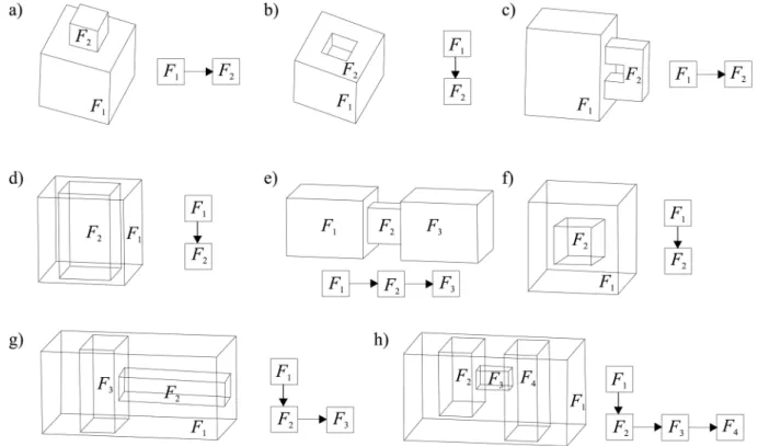
and each of these rings is said to open the fea-tureFon the surface. According to the number of rings, we distinguish between:
DP–features, which define a single ring. Representatives of this class arean explicit protrusion(Fig. 1a)andan explicit
depres-sionora pocket(Fig. 1b).
H–features, which define two or more rings on one or more faces of the object. These faces can belong to different features of the object. A handle (Fig. 1c) is fastened to
a single feature, and a through–hole (Fig.
1d)tunnels just one feature as well. Two or
more features can be connected bya bridge
(Fig. 1e).
Algorithms for explicit feature recognition usu-ally complete features with missing faces. In this way, each feature becomes a regular geo-metric solid. An algorithm should create a new face for each ring, and the observed ring be-comes the external loop of the new face. How-ever, in the resulting collection of regular 3D shapes, there are also features, which have not
defined any rings in the past. We name them main shapes. Only the topological data suf-fices for the object decomposition and classi-fication of extracted features into main shapes, DP–features and H–features, but such topolog-ical algorithms are typtopolog-ically used only as pre-processors to geometric algorithms that further classify features from particular classes into ex-ternal and inex-ternal. This geometic classifica-tion is usually done by determining convexity of edges forming the rings7]. External features
are protrusions, handles and bridges, and inter-nal are pockets and through–holes. An interinter-nal equivalent to the bridge is calleda bridge be-tween internal features(Fig. 1g and Fig. 1h).
The main shape can also be either external or internal. The latter is called a void (Fig. 1f).
The meaning of the hierarchical structures in Fig. 1a–h will be described later.
The second category consists of implicit fea-tures. They are not based on rings, but on con-cave edges of external loops. Algorithms for their recognition are projected on geometrical data. The task of testing convexity of edges can be transformed into the problem of face orien-tation(determining the exterior and the interior
side of the face). An implicit depression is
Fig. 2.A shape with an implicit a)depression, b)protrusion.
shown in Fig. 2a, and an implicit protrusion can be seen in Fig. 2b.
3. Algorithm for Recognition of Explicit Geometric Features
The basic idea of the presented algorithm can be employed on any geometric shape, but the cur-rent implementation of some supporting func-tions enables only feature recognition in scenes with planar faces. Explicit features being recog-nised can be opened by arbitrary number of rings, and these can belong to different features. But a ring is allowed to be defined on a single face of a feature only. This feature is said to be external to the feature opened by the ring. The limitation means that features expanding through more faces like a protrusion on an edge cannot be recognised.
The method is not based on usual division to external and internal features. The features are rather classified asfilled (by material)and
empty features. This proves sensible when nested features are present. Namely, it sounds strange and confusing that some external fea-ture could be included in an internal one. The method operates in two phases:
a topological partcompletes the model with new faces encircled by rings, divides the scene into simpler valid geometric bodies
(features), and classifies these features into
four classes: main shapes, DP–features, H– features attached to a single feature, and H–features connecting more features. Only topological data are employed.
a geometrical partclassifies extracted fea-tures into filled and empty ones. Each of four classes is split into two new classes. The classification is not being executed by testing convexity of edges in rings, but rather by determining eventual mutual containment of features. The problem of penetration is partially handled, too.
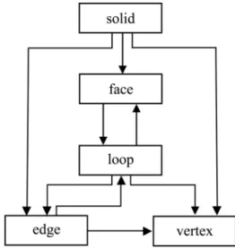
Besides the geometrical and topological data, the employed boundary model includes fields that characterise features, and some additional information for the program control. A solid is presented by faces, loops, edges and vertices as shown in Fig. 3. Arrows indicate accessi-bility of entities of a particular type. Three lists of geometric elements are directly accessi-ble through the solid object: faces, edges and vertices. However, loops cannot be reached directly but through faces (the relation face–
loop). Multiple connected faces are encircled
by several loops. In the data structure, they are organised in a double–connected list. The first list element presents the external loop. It can be followed by several elements presenting eventual rings. After the decomposition, the face–loop relation becomes one–to–one, and we do not have to distinguish between both entity types any more. The inverse relation loop–face enables us to access both elements simultane-ously. Loops are also accessible through edges. The relation edge–loop could seem a bit strange or at least redundant to someone, but it speeds up some parts of the program considerably.
4. Topological Part of the Algorithm
In the first part of the algorithm, the feature extraction and the first step of the feature clas-sification are done. The employed topologi-cal algorithm is just an adaptation of the algo-rithm described by De Floriani and Bruzzone7]
with some modifications of the data structures. While only the topological data are employed, this step works successfully with objects with non–planar faces as well. The feature extraction is carried out in two steps:
Creation of new faces – new face is created for each ring, and the ring becomes its external loop. At the same time, it is removed from the list of loops of previously multiple connected face. This face is said to be external to the newly created face. After the removal of all rings, we obtain the set of simply connected faces. Object decomposition – the scene is decom-posed into features with regard to adjacency of edges and vertices only. The features are simpler bodies bounded by simply connected faces only. In the first part of the decomposi-tion, each face is tested against all faces situ-ated in the face list before it. The test searches for faces that share common edges and there-fore belong to the same feature. Such faces are called combinable. The same term is used for the feature candidates that should be joined. Al-though all necessary information are accessible directly from the boundary representation, some additional fields in the data structure speed up the process considerably. The description of the face is extended by the fieldsfeature IDand
edge set. Two arrays of integers: combinable
and correction are also employed in this step.
They refer to feature candidates, and the current number of them is stored innumber of features, which may not exceed the predefined constant
max features. Theedge sethas to be initialised
with indices of all edges of the external loop of the corresponding face i.e. with their relative positions in the edge list, and all fieldsfeature ID have to be set to some value larger than the real number of features (max features + 1). Three
different situations can occur during testing a face against preceding members of the face list:
(i) The face currently being tested is not
com-binable with any other face. New feature candidate is identified. Thenumber of featu-res is incremented by one, and the fields
combinable[number of features]andcorrection
[number of features]are employed then.
Whi-le such a face and a corresponding feature are not combinable with any other identified since that moment, the value of combinable is set to its index.
(ii)The tested face ftis combinable with a face
fpbelonging to the feature indexedi, and ft
is already combinable with some other face belonging to the featurej, wherej<i. The
following actions have to be performed:
f[t].edge set =S
(f[t].edge set, f[p].edge set);
f[p].edge set = f[t].edge set
combinable[f[p].feature ID] = f[t].feature ID;
(iii)The face currently being tested(ft)is
com-binable with a face fpbelonging to the
fea-turei, and ft has not been combinable with
any face yet, or it is eventually combinable with some face belonging to the feature j, wherej>i. The following actions have to
be performed:
f[t].edge set=S
(f[t].edge set, f[p].edge set);
f[p].edge set = f[t].edge set
f[t].feature ID = combinable[f[p].feature ID];
It is obvious that the values combinable are forced to become as low as possible. They are initialised with their indices and later, they can be only decreased. We are especially interested in those fields that keep their values unchanged after all comparisons. These fields actually present real features, and will be called feature– introducing elements (FIEs). Currently, each
face is assigned to one ofnumber of features fea-ture candidates, but we want them all assign to the FIEs only. The number of features should present number of FIEs, and indices of FIEs have to be transformed into the range [1,
num-ber of features].
In the continuation, we first calculate correc-tions of indices of FIEs and the correct
num-ber of features. Then we find the FIE and repair
are given below. Finally, we are ready to per-form the real object decomposition by splitting common lists of faces, edges and vertices into partial ones describing particular features. At this stage, we can already initialise some aux-iliary data refering to the features: coordinates of the bounding box needed for the minimax test in the geometrical part of the algorithm, the number of newly created faces of the feature
(number of rings), and the number of features
that contain the rings describing these newly created faces(number of parents).
Algorithm FindFIE (face,fie)
begin
fie = combinable[face.feature ID];
loop
if (fie = combinable[fie]) then exit loop;
fie = combinable[fie];
forever; end.
...
(* calculate correct feature ID of face f *)
FindFIE (f,fie);
f.feature ID =fie correction[fie]; ...
Feature extraction is followed by a topologi-cal part of the feature classification. In the feature’s data structure there is also the inte-ger variable feature class, which is set to value between 1 and 4:
1 – main shape
(number of rings = number of parents = 0),
2 – DP–feature
(number of rings = 1),
3 – H–feature on one feature
(number of rings>1, number of parents = 1),
4 – bridge
(number of parents>1).
An example of feature extraction and topologi-cal classification is given in an appendix.
5. Geometrical Part of the Algorithm
The topological algorithm represents a prepro-cessor for geometric classification. We cannot
imagine an application that would treat a de-pression or protrusion, for example, in the same way. If the manufacturing machine obtains in-formation to process a DP–feature, it "does not know" whether to remove the interior or the exterior of the feature. Most common geomet-rical classification distinguishes between exter-nal and interexter-nal geometric features. The clas-sification usually tests concavity of the edges forming rings, and meet the complex problem of face orientation14]. As long as main shapes
are supposed to be filled by material, the prob-lem is solved easily, but it becomes a hard one if voids are allowed. A protrusion on void does not define a concave, but a convex edge. Before performing any tests of concavity of edges, the differentiation of filled and empty main shapes has to be done. In addition to this, we allow fea-tures nested to arbitrary level to increase gen-erality and applicability of the method. There-fore, a hierarchical structure connecting main shapes according to their eventual mutual con-tainment is employed. Features not contained in any other feature are placed at the root level, and at the leveln, we meet the features directly contained in the features of the leveln;1.
Fea-tures placed at odd levels are identified as filled, and those at even level are empty features. How-ever, voids can be contained in any filled feature and not only in main shapes. For this reason, all the features should be arranged in the hier-archical structure, and therefore, they can also be classified according to odd or even level of appearance. Before describing the details, the main procedure of the geometrical part of our algorithm is listed.
Algorithm ClassifyFilledEmpty() begin
elt = CreateNode(1); rootNode = elt; j = 2;
loop
if (j>number of features) then exit loop;
elt = CreateNode(j);
rootNode = InsertNodeToStructure(elt, rootNode); j = j + 1;
forever;
ClassificationOddEven(rootNode, 1);
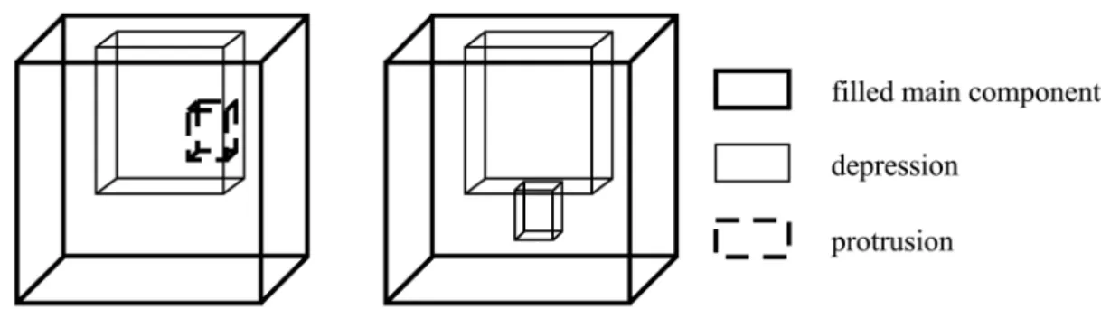
Fig. 4.Left: depression in depression is protrusion. Right: nested depression.
5.1. Relation of Containment
FunctionInsertNodeToStructurepresents the only point where the algorithm meets geometrical data. Namely, determination of eventual fea-ture intersections and the containment test are hidden inside its body. We suppose that only an empty feature can be directly contained in the filled one and the opposite, the filled feature always occupies some empty space and not the space occupied by some other filled feature. In this way, we obtain the desired result: empty features are at even levels in the hierarchical structure, and filled features are at odd levels. A depression in a depression has to be recog-nised as protrusion, and a nested depression is still a depression. Both examples are shown in Fig. 4.
The containment test has to identify whether the tested feature is situated inside another fea-ture or not. We use a 3D extension of simple containment test point–in–polygon to find out whether the point is inside the body or not15].
While the test is performed after handling pos-sible feature intersections, it suffices to test a single point of the tested feature against all faces of the other feature. Unnecessary calculations can be avoided by performing a simple minimax test.
5.2. Auxiliary Hierarchical Structure
Geometrical classification is facilitated by em-ploying the hierarchical structure connecting nodes(features)according to their mutual
con-tainment or intersections. Two nodes at the same level are not contained in each other, and will be calledsiblings. The featureFicontained
in some other feature Fj is recursively inserted
into the substructure rooted inFj, among the
de-scendantsofFj. Direct descendants are called
sons. Analogously, nodes that contain some other node(Fi)are calledancestorsofFi.
Di-rect ancestor isfather. Each node, except the ones at the root level, has exactly one father. Nodes are accessible through the ancestors, and the inverse connections are not defined. The number of sons is arbitrary, but in the struc-ture, only a pointer to one of them is used. All its siblings are listed behind it in the connected list. Each list is connected in one direction only, and therefore, we shall distinguish between left and right siblings. When we reach a particular node, its left siblings have been visited already, and the right siblings and the descendants of the node form the substructure that should be vis-ited next. Each node contains the pointer to the first node in the list of its sons (first son), the
pointer to the next right sibling(first sibling)and
the fieldfeature IDthat establishes a unique re-lation between the node and the corresponding feature obtained in the topological part.
In Fig. 1 already, all types of features recognised by our algorithm and the corresponding hierar-chical structures are given. Horizontal connec-tions present siblings, and the vertical are used for father–son relations. Unfortunately, this simple organisation is useful only while feature intersections are not allowed. When we meet a featureFithat is partially contained inside some
other featureFj, and the rest ofFiis outsideFj,
then we cannot decide whether to insert the cor-responding node Fi between the siblings ofFj
5.3. The Problem of Feature Intersections
When we talk about general and really usable algorithm, we cannot avoid the problem of fea-ture intersections. Possible appearance of in-tersections of solid bodies presents one of the main problems in computer graphics and geo-metric modelling. In our algorithm, only the real scenes are expected. Filled feature can be directly(partially)contained only in an empty
feature, and similarly, empty feature can be di-rectly partially contained in a filled one only. We rather use the termpartial containment in-stead of feature intersection to show that one feature is pierced by another in such situation. The node of featureFipiercing the featureFjis
cloned, and the original is inserted among the sons ofFj, and the copy is inserted into the list
of right siblings of Fj. The first copy is
pre-senting a part ofFi that is contained inFj, and
the second copy is used for the part of Fi
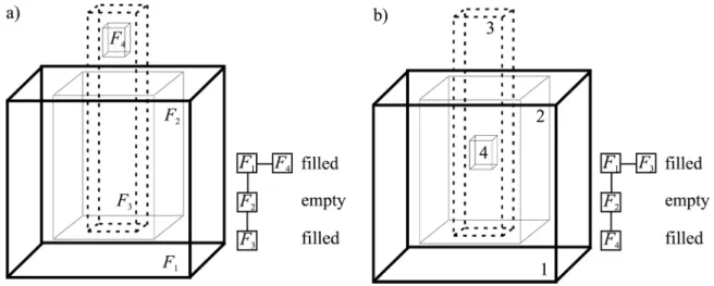
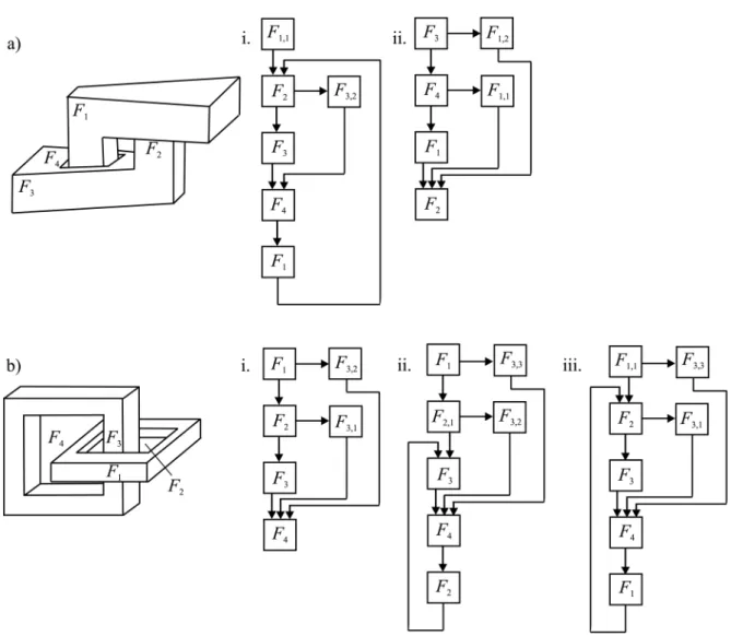
out-side Fj. After study of both examples in Fig.
5, the reader will understand why two copies of the protrusionF3 are necessary. In case a),
the protrusion is placed among descendants of the main shapeF1and the depressionF2 only,
and the void F4, which is situated outside the
main shape F1, is incorrectly classified as the
filled feature. In case b), the protrusion F3 is
inserted to the list of siblings of the main shape
F1, and the voidF4between the descendants of
the featureF1. The voidF4is again incorrectly
recognised as filled feature.
Possible intersections are determined by search-ing for the intersections of the faces belongsearch-ing
to the first feature and those belonging to the second one. If two faces are intersecting, the procedure can be released. While the polygons presenting faces can be concave as well, it does not suffice to test only two line segments, but to find all intervals on line obtained as the inter-section of two planes. It is wise to employ the test minimax. If the intersection is not identi-fied after testing all pairs of intervals, the next pair of faces is being tested. If no intersections are identified after all possible tests, the con-tainment test can be employed on the same pair of features.
5.4. Creating the Hierarchical Structure
Two functions are employed to create the hier-archical structure. The simple one named
Crea-teNode(int j)creates the node presenting the
fea-ture Fj, and the second one
InsertNodeToStruc-ture(elt, rootNode)recursively inserts the nodeelt
into the substructure with rootrootNode. The hi-erarchical structure should be organised in the way that all the copies presenting the same fea-ture have common sons, but different siblings. Six different situations can occur while insert-ingeltin the structure:
1. SubstructurerootNodeis empty. The nodeelt becomes the root of the substructure. 2. Feature elt is piercing the feature rootNode.
Nodeeltis recursively inserted into the sub-structure of the descendants ofrootNode. If elt is not a sibling of the rootNode yet (the
Boolean field visited is employed for this task), a copy of eltis inserted into the
sub-structure of right siblings ofrootNode. 3. The noderootNodeis piercing the new node
elt. The rootNode is cloned, and a copy is inserted in the structure of descendants of elt. The node elt occupies the place of the
rootNodein the structure, another copy of the
rootNode is inserted in the structure of right
siblings ofelt, and all the previous right sib-lings of therootNodeare recursively inserted into the substructure with the new root node elt.
4. New node elt is contained in the root root-Node. The node elt is recursively inserted into the structure of descendants ofrootNode. 5. The noderootNodeis contained in new node elt. TherootNodeis cloned, and a copy is in-serted in the structure of descendants ofelt. The node eltoccupies the place of the
orig-inalrootNode, and all the previous right
sib-lings of therootNodeare recursively inserted into the substructure with the new root node elt.
6. New node elt and the root of the structure
rootNode do not intersect and are not
con-tained in each other as well. The node elt is recursively inserted into the structure of right siblings ofrootNode.
5.5. Geometrical Classification to Filled and Empty Features
The nodes at odd levels are presenting filled fea-tures and the nodes at even levels correspond to empty features. Each node contains the integer attributefeature IDthat enables direct access to the data structure presenting the feature. We remember that the topological part has set the value feature classin this structure to the inte-ger number between 1 and 4. The geometrical classification only changes the sign of the
fea-ture classfor all features with the corresponding
nodes at even levels of the hierarchical structure. In this way, we split each of the four classes into two new classes, and therefore, obtain eight fea-ture classes. But the problem appears because multiple copies presenting the same feature can be located at both, odd and even levels. Without mathematical proof, we shall declare that in the
depth–first search of the structure, the first copy
(the left–most copy)of the node met is correctly
nested. For both examples from Fig. 5, we ob-tain the structure shown in Fig. 6. The left most copy of the protrusionF3is correctly nested at
the third(odd)level. Right copiesF3 1andF3 2
are not tested, and therefore, the incorrect even level of the nodeF3 1 does not have any
influ-ence to the solution. The common descendant of all three copies(voidF4)is met after visiting
the left most copy of its fathers, and it is again correctly set at the fourth(even)level.
Fig. 6.Incorrect level of the right copy(F3 1)does not affect the solution.
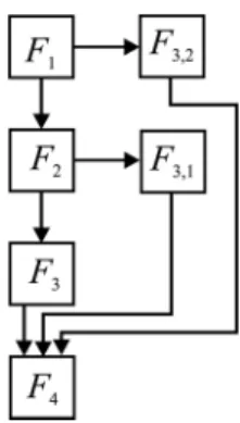
In Fig. 7, two more complex examples are given. In both cases, we meet the same problem: the existance of features that are pairly intersecting each other, and we cannot specify which one is the piercing feature and which is the pierced one. While the algorithm can only handle this type of feature intersections, it simply chooses one of the intersecting features to be the pierc-ing one and another to be the pierced feature. The choice depends on indices of features and also on ordering of faces of both features. How-ever, we have tested all possible orders of fea-tures for both examples, and the obtained results were correct in all cases: the left most copies of solid features are situated at odd levels, and the left most copies of empty features can be met at even levels only.
In the example a), we have two solid main
shapes and each of them contains a depression. Four features can be ordered in 4!= 24
Fig. 7.Two more examples of pairs of components piercing each other.
higher index, and the opposite. Therefore, 24 situations have to be observed. Two of them corresponding to indexing, applied in the fig-ure, are presented. The structure i)corresponds
to the case when the solidF3is the piercing one,
and the structure ii)was obtained when the solid
F1was piercing the solidF3and the pocketF4.
The example b) is even more complex. We
have two solid main shapes, and each of them contains a through–hole. Again, we have 24 different ways of feature indexing, but because of the symmetry, only 12 of them are interest-ing. But this time, both, the solid feature and its nested through–hole are simultaneously pierc-ing another solid feature and a through–hole, and the opposite. Altogether, we had to test 122
4
=192 situations and we always obtained
correct result.
In all hierarchical structures, the original nodes are labeled F1, F2, F3, F4, and copies are
equipped with additional indices regarding the time of their creation(the copy created earlier
has lower index). By observing the
hierachi-cal structures in Fig. 7 carefully, a conclusion can be made that the nodes can be perturbed sev-eral times during the creation of the hierarchical structure. In the case b.iii), the nodeF1 1which
was created as the right copy, even became the root node, and therefore, the left most copy of the nodeF1. The main reason for these
0 – the featuresFiandFjhave not been tested
yet,
1 – the featureFicontains the featureFj,
2 – the featureFjcontains the featureFi,
3 – the featureFiis piercing the featureFj,
4 – the featureFjis piercing the featureFi,
5 – featuresFiandFjdo not contain each other
and do not intersect.
Of course, only the pairs of features, where both corresponding matrix elements are set to 0, have to be tested, what accelerates the program con-siderably.
6. The Time Complexity
The time complexity of the algorithm varies from step to step and does not exceed O(n
2
).
In the topological part, a new face is created for each ring of multiple connected faces at the beginning. We obtain linear time complexity
O(n), where n is the number of rings. In the
object decomposition step, each face is tested against all faces situated in the face list before it. We haven(n;1)=2 comparisons, and this
gives the time complexity O(n
2
), where n is
the number of faces. Corrections of indices of FIEs are then calculated inO(n), wherenis the
number of feature candidates. After this, the FIE for each face should be determined. Let us suppose that we have a single feature, and an inconvenient order of its faces causes that each face is attached to different feature can-didate. Fortunately, this is not possible, and the time complexity of this step cannot exceed
O(n
2
). At the end of the object decomposition
step, each face, edge and vertex is assigned to the corresponding feature. Each list element is visited once, and we obtain the time complexity
O(n). The topological classification is also
ex-ecuted inO(n), wherenis the number of faces
(the feature’s attributes depend on attributes of
the feature’s faces). The time complexity of the
geometrical part depends a lot on the branch-ing of the hierarchical structure. In the worst case, we have to test each feature being inserted against all other features in the structure, and we obtainn(n;1)=2 comparisons.
7. Conclusions
In the paper, the algorithm for explicit fea-ture extraction and classification from bound-ary representation is presented. It operates in two phases: the topological and the geometri-cal, and classifies extracted features into eight classes. The topological part is not limited to the bodies with planar faces, but in the geomet-rical part, the current implementation of some tasks requires this limitation. It can be omit-ted by approximation of curved faces by sets of planar polygons and by performing the con-tainment test and the feature intersection test on these polygons.
The last version of the algorithm is implemented in C++and is going to be integrated with the
geometric constraint solver into an efficient tool for manipulation of mechanical parts. Let us suppose that we have a protrusion placed exactly in the middle of the top face of the block(main
shape). If we change the dimensions of the
block, it is hard to believe that the protrusion is still placed in the middle. The geometrical data describing the protrusion have to be manually updated to satisfy this requirement. This is just a simple example, but in practise, hundreds or thousands of calculations should be performed to enable such modifications of the geometry preserving additional requirements of the rela-tive positions of the features. This is the ideal task for employing geometric constraints. But remember that first we have to obtain geometric features from the original boundary representa-tion in some way, and this is the funcrepresenta-tion of the algorithm described in the paper.
Beside to generalisation of the algorithm to han-dle objects with non–planar faces, and integra-tion of the feature–based and constraint–based design, our future work is intended to introduce new explicit feature types containg rings opened on two or more neighbouring faces.
APPENDIX
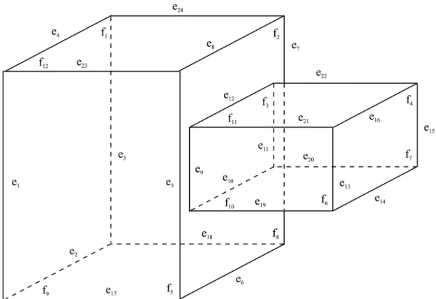
Let us highlight the object decomposition and topological classification(Section 4)on a
sim-ple examsim-ple described in Fig. 8. Left and right vertical faces are denotedf1– f4, front and back
Fig. 8.Example illustrating object decomposition.
f9– f12. The faces are indexed in order of their
appearance in the face list. The initial data are shown in Tab. 1.
face edge set feature ID
1 1–4 1001
2 5–8 1001
3 9–12 1001
4 13–16 1001
5 1, 5, 17, 23 1001
6 9, 13, 19, 21 1001
7 11, 15, 20, 22 1001
8 3, 7, 18, 24 1001
9 2, 6, 17, 18 1001
10 10, 14, 19, 20 1001 11 12, 16, 21, 22 1001
12 4, 8, 23, 24 1001
Tab. 1.The initial data for the object decomposition example.
While the faces f1 – f4 do not share any
com-mon edges, they are assigned to four different features(Tab. 2 and Tab. 3).
face edge set feature ID
1 1–4 1
2 5–8 2
3 9–12 3
4 13–16 4
Tab. 2.Changes after testing facesf1–f4.
feature combinable
1 1
2 2
3 3
4 4
Tab. 3.Feature candidates after testing facesf1–f4.
The face f5 shares the edgee1with the face f1,
and therefore belongs to the featureF1 (
situa-tion iii). While it also shares common edgee5
with face f2, the feature F2 is identified
com-binable with the featureF1(see Tab. 4 and Tab.
face edge set feature ID
1 1–5, 17, 23 1
2 1–8, 17, 23 2
5 1–8, 17, 23 1
Tab. 4.Changes after testing facef5.
feature combinable
1 1
2 1
Tab. 5.Feature candidates after testing facef5.
Similarly, face f6shares common edgee9 with
the face f3, and therefore belongs to the feature
F3 (situation iii). It also shares edge e13 with
face f4, and the featureF4is identified
combin-able with the featureF3(Tab. 6 and Tab. 7).
face edge set feature ID
3 9–13, 19, 21 3
4 9–16, 19, 21 4
6 9–16, 19, 21 3
Tab. 6.Changes after testing facef6.
feature combinable
3 3
4 3
Tab. 7.Feature candidates after testing facef6.
The face f7is combinable with faces f3, f4and
f6 as well, while we rewrite sets of edges with
unions of two sets. Similarly, the facef8is
com-binable with faces f1, f2 and f5. The situation
in Tab. 8 and Tab. 9 is obtained.
face edge set feature ID
1 1–5, 7, 17, 18, 23, 24 1
2 1–8, 17, 18, 23, 24 2
3 9–13, 15, 19–22 3
4 9–16, 19–22 4
5 1–8, 17, 18, 23, 24 1
6 9–16, 19–22 3
7 9–16, 19–22 3
8 1–8, 17, 18, 23, 24 1
Tab. 8.Changes after testing facesf7andf8.
feature combinable
1 1
2 1
3 3
4 3
Tab. 9. Feature candidates after testing facesf7andf8.
After testing all horizontal faces f9 – f12 we
finally obtain the situation in Tab. 10 and Tab. 11.
face edge set feature ID
1 1–8, 17, 18, 23, 24 1
2 1–8, 17, 18, 23, 24 2
3 9–16, 19–22 3
4 9–16, 19–22 4
5 1–8, 17, 18, 23, 24 1
6 9–16, 19–22 3
7 9–16, 19–22 3
8 1–8, 17, 18, 23, 24 1
9 1–8, 17, 18, 23, 24 1
10 9–16, 19–22 3
11 9–16, 19–22 3
12 1–8, 17, 18, 23, 24 1
Tab. 10.Situation after testing all facesf1–f12.
feature combinable
1 1
2 1
3 3
4 3
Faces are assigned to four different features, but only two of them are FIEs: the feature F1 and
F3have valuescombinableequal to their indices.
The former does not need any corrections, but for the featureF3, thecorrectionis set to 1 while
it is preceded by one feature (F2) combinable
with some other. Thenumber of featuresis set to 2. Now, we find the FIE for each face. Finally, we calculate the correct values offeature IDfor each face, and physically divide lists of faces, edges and vertices.
Faces f1, f2, f5, f8, f9, f12and the
correspond-ing edges and vertices are assigned to the feature
F1, and all the rest to the feature F2. The
num-ber of rings for the feature F2 is set to 1 while
the face f3was created from the ringe9–e10–
e11–e12, and thenumber of parentsis set to 1 as
well. For the feature F1, both values are zero.
The featureF1is therefore recognised as a main
shape, and the featureF2is a DP–feature.
References
1] B. FALCIDIENO ANDF. GIANNINI, Automatic Recog-nition and Representation of Shape–Based Features in a Geometric Modeling System,Computer Vision, Graphics and Image Processing, No. 48(1989), pp. 93–123.
2] J. R. WOODWARK, Some speculations on feature recognition,Computer–Aided Design, Vol. 20, No. 4, 1988, pp. 189–196.
3] J. C. E. FERREIRA ANDS. HINDUJA, Convex hull– based feature–recognition method for 2.5D com-ponents,Computer–Aided Design, Vol. 22, No. 1, 1990, pp. 41–48.
4] D. SANDIFORD AND S. HINDUJA, Construction of feature volumes using intersection of adjacent sur-faces,Computer–Aided Design, Vol. 33, 2001, pp. 455–473.
5] S. MEERAN, J. M. TAIB, A generic approach for recognising isolated, nested and interacting features from 2D drawings, Computer–Aided Design, Vol. 31, No. 14, 1999, pp. 891–910.
6] L. DE FLORIANI, Feature Extraction from Boun-dary Models of Three–Dimensional Objects,IEEE Transactions on Pattern Analysis and Machine In-telligence, Vol. 11, No. 8, 1989, pp. 785–798.
7] L. DEFLORIANI, E. BRUZZONE, Building a feature– based object description from a boundary model,
Computer–Aided Design, Vol. 21, No. 10, 1989, pp. 602–610.
8] R. ANANTHA, G. A. KRAMMER,ANDR. H. CRAW-FORD, Assembly modelling by geometric constraint satisfaction,Computer–Aided Design, Vol. 28, No. 9, 1996, pp. 707–722.
9] B.ZALIK, N. GUID, An approach to applying con-ˇ straints in geometric modelling, Journal of Com-puting and Information Technology, Vol. 3, No. 4, 1995, pp. 229–244.
10] D. PODGORELEC, A new constructive approach to constraint–based geometric design, Computer– Aided Design, Vol. 34, No. 11, 2002, pp. 769–785.
11] K. MARTINI, Hierarchical geometric constraints for building design,Computer–Aided Design, Vol. 27, No. 3, 1995, pp. 181–191.
12] J. K. GUI ANDM. M¨ANTYLA, New concepts for¨ complete product assembly modeling, ACM digital library, Proceedings of the Second symposium on solid modeling and applications, 1993, pp. 397– 406.
13] M. E. MORTENSON,Geometric Modeling, John Wi-ley, New York, 1985, 763 pp.
14] P. GAVANKAR, M. R. HENDERSON, Graph–based ex-traction of protrusions and depressions from bound-ary representations,Computer–Aided Design, Vol. 22, No. 7, 1990, pp. 442–450.
15] J. D. FOLEY, A. VAN DAM, S. K. FEINER, J. F. HUGHES, Computer Graphics — Principles and Practise, 2nd ed., Addison–Wesley, Reading, 1990, 1174 pp.
Received:June, 2001
Revised:October, 2002
Accepted:December, 2002
Contact address:
David Podgorelec Faculty of Electrical Engineering & Computer Science University of Maribor Smetanova 17, 2000 Maribor, Slovenia. e-mail:[email protected]
DAVIDPODGORELECreceived the BSc degree, MSc degree and PhD in computer science from the University of Maribor, Slovenia, in 1993, 2000 and 2002, respectively. He is a lecture assistant in the department of Computer Science, Faculty of Electrical Engineering & Computer Science(EE&CS), University of Maribor, Slovenia. His research in-terests include constraint–based and feature–based geometric design, computational geometry, visualisation of medical data, and multimedia applications.