Vol. 5, No. 2, 2012, 211-249
ISSN 1307-5543 – www.ejpam.com
Misspecified Multivariate Regression Models Using the Genetic
Algorithm and Information Complexity as the Fitness Function
Hamparsum Bozdogan
1,∗, J. Andrew Howe
21 Department of Statistics, Operations, and Management Science, The University of Tennessee,
Knoxville, TN, 37996, USA
2TransAtlantic Petroleum, Business Analytics, Istanbul Turkey
Abstract. Model misspecification is a major challenge faced by all statistical modeling techniques. Real world multivariate data in high dimensions frequently exhibit higher kurtosis and heavier tails, asymmetry, or both. In this paper, we extend Akaike’sAI C-type model selection criteria in two ways. We use a more encompassing notion of information complexity (I COM P) of Bozdogan for multivariate regression to allow certain types of model misspecification to be detected using the newly proposed criterion so as to protect the researchers against model misspecification. We do this by employing the “sandwich”or “robust”covariance matrixFˆ−1RˆFˆ−1, which is computed with the sample kurtosis and skewness. Thus, even if the data modeled do not meet the standard Gaussian assumptions, an appro-priate model can still be found. Theoretical results are then applied to multivariate regression models in subset selection of the best predictors in the presence of model misspecification by using the novel genetic algorithm (GA), with our extendedI COM Pas the fitness function.
We demonstrate the power of the confluence of these techniques on both simulated and real-world datasets. Our simulations are very challenging, combining multicolinearity, unnecessary variables, and redundant variables with asymmetrical or leptokurtic behavior. We also demonstrate our model selec-tion prowess on the well-known body fat data. Our findings suggest that when data are overly peaked or skewed - both characteristics often seen in real data, I COM P based on the sandwich covariance matrix should be used to drive model selection.
2010 Mathematics Subject Classifications: 62H86, 62J05, 62N02, 65G20, 62-07, 62F12, 62E20, 81T80, 78M34, 62B10
Key Words and Phrases: Misspecified multivariate regression models, Information complexity, Robust estimation, Genetic algorithm, Subset selection, Dimension reduction
1. Introduction
Model misspecification is a major, if it is not the dominant, source of error in the quantification of most scientific analysis- Chatfield, 1995.
∗Corresponding author.
Email addresses:bozdoganutk.edu(H. Bozdogan),ahowe42gmail.om(J. Howe)
In this research article, we simultaneously address several issues that affect many sta-tistical modeling procedures. Specifically, this paper deals with the context of multivariate regression (MVR).
Statistical models are typically merely approximations to reality; additionally, for a set of observations, we typically don’t know the true data generating process. Therefore, a wrong ormisspecified modelhas a high probability of being fit to observed data. In many real-life ap-plications of strategic decision making, large numbers of variables need to be simultaneously considered to build anoperating modeland for real-time data-mining. Application examples would include
• Behavioral and social sciences, • Biometrics,
• Econometrics,
• Environmental sciences, and • Financial modeling.
Further, it is often the case that several response variables are studied simultaneously given a set of predictor variables. In such cases it is often desirable to:
• determine whichsubsets of the predictorsare most useful for forecasting each response variable in the system,
• interpret simultaneously a large number of regression coefficients, since this can become unwieldy even for a moderately-sized data, and
• achieve parsimony of unknown parameters, allowing both better estimation and clearer interpretation of the parameters.
Our objectives are twofold. The first is to develop acomputationally feasible intelligent data mining and knowledge discovery technique that addresses the potentially daunting statistical and combinatorial problems of MVR modeling under model misspecification. Secondly, we provide new research tools that guide model fit and evaluation for high dimensional data, regardless of whether or not the probability model is misspecified. We employ a three-way hybrid:
• Our approach integrates novel statistical modeling procedures based on a misspecification-robust form of theinformation complexity (I COM P) criterion[5, 4, 6, 7]as the fitness function;
• Multivariate regression models that allow for non-Gaussian random errors, and
• The genetic algorithm(GA) as our optimizer to select the best subset of predictors or variables.
To this end, we developed an easy-to-use command- and GUI- driven interactive computa-tional toolbox. With this MATLAB®toolbox, we illustrate our new approach on both real and simulated data sets, showing the versatility of these techniques.
respectively. The basic idea is that one can use the difference betweenI COM P(misspecified model) and I COM P(correctly specified model) as an indication of possible departures from the distributional form of the model. This brings out the most important weakness of Akaike-type criteria for model selection: these procedures depend crucially on the assumption that the specified family of models includes the true model. We also propose a penalty-bias func-tion under the distribufunc-tional misspecificafunc-tion. In Secfunc-tion 4, we provide the explicit expression ofI COM P for the correctly specified as well as for misspecified multivariate regression model and we derive the bias of the penalty for the misspecified multivariate regression model under normality. This form is useful in obtaining the amount of bias, based on maximum-likelihood estimation when distributional (or other) assumptions are not satisfied. The resulting penalty-bias function turns out to be a function of skewness and kurtosis coefficients. Next, in Section 5 we provide details of the genetic algorithm (GA) and robust covariance estimators (Section 6). Finally, results with both simulated and real datasets are shown in Section 7, followed by concluding remarks. In Appendices 1 through 3, we repeat the analytical matrix calculus derivations of the model covariance matrix for multivariate regression under misspecification, based on the work of [27], for the benefit of the readers. Much of this work was done in collaboration with the first author while he was a Senior Scientist at Tilburg University, in Tilburg, the Netherlands during May of 1999. In Appendix 1, we show the derivation of the outer-product form of the Fisher information matrix. In Appendix 2, we show the derivation of the sandwich model covariance matrix which is a new result in closed-form which does not exist in the literature within the context of a misspecified MVR model. The opened up form of the misspecification resistant I COM P is obtained and shown, and Appendix 3 derives the penalty bias for multivariate regression.
2. Multivariate Gaussian Regression (MVR) Model
In the usual well known multivariate regression problem, we have a matrix of responses Y ∈Rn×p;nobservations ofp measurements on some physical process. The researcher also
haskvariables that have some theoretical relationship toY: X ∈Rn×q, of course, we usually
include a constant term as an intercept for the hyperplane generated by the relationship, soq = k+1. The predictive relationship between X and Y has both a deterministic and a stochastic component, such that the model is
Y =X B+E, (1)
in whichB∈Rq×p is a matrix of coefficients relating each column ofX to each column ofY,
and E∈Rn×p is a matrix of error terms. The usual assumption in multivariate regression is that the error terms are uncorrelated, homoskedastic Gaussian white noise, or
E∼Np(0,Σ⊗In), (2)
where the entire covariance matrix of the random error matrix Eis given by
This is an(np×np)matrix, where⊗denotes the direct or Kronecker product. Stated another way, we require
Y ∼Np(X B,Σ⊗In), (4)
where
E(Y) =X B, andC ov(Y) = Σ⊗In. (5) Under the assumption of Gaussianity, the log likelihood of the multivariate regression model is given by
logL(θ|Y) =−np
2 log(2π)− n
2log|Σ| − 1
2tr[(Y−X B) Σ
−1(Y−X B)′]. (6)
We obtain quasi maximum-likelihood estimators ofBandΣby maximizing the log-likelihood function in (6). From[28, page 321], the first differential of the log-likelihood is
d logL(θ|Y) = −n
2trΣ
−1dΣ +1
2tr[(Y−X B)Σ
−1(dΣ)Σ−1(Y−X B)′]
+trX(dB)Σ−1(Y−X B)′
= 1
2tr(Σ
−1(Y−X B)′(Y −X B)Σ−1−nΣ−1)dΣ
+trΣ−1(Y−X B)′XdB, (7)
leading to the first-order conditions
Σ−1(Y−X B)′(Y−X B)Σ−1=nΣ−1, andX′(Y−X B)Σ−1=0, (8) and hence to the quasi maximum-likelihood estimators ofB andΣgiven by
ˆ
B= (X′X)−1X′Y, (9)
and
ˆ Σ = 1
n(Y−XBˆ)
′(Y−XBˆ) = 1
nEˆ ′Eˆ= 1
nY
′M Y, (10)
where M=I−X(X′X)−1X′is an idempotent matrix.
To derive the information complexity (I COM P) criteria, we modify the results of[28, page 321], and obtain the estimatedinverse Fisher information matrix(IFIM) given by
Ô
C ov(vec( ˆB), vech( ˆΣ))≡Fˆ−1=
ˆ
Σ⊗(X′X)−1 0 0′ 2nD+p( ˆΣ⊗Σ)ˆ D+p′
, (11)
where D+p = (D′pDp)−1Dp is the Moore-Penrose inverse of the duplication matrix,Dp. Dp is a uniquep2×12p(p+1)matrix that transforms, for symmetricΣ, vech(Σ)into−→Σ. For example, forp=2,
−→
where the supradiagonal elementσ12 has been removed. Thus, for symmetric Σ, vech(Σ) only contains the distinct elements ofΣ. That is,
Dpvech(Σ) =−→Σ,(Σ = Σ′). For an excellent treatment ofDp, see[26].
The IFIM provides the asymptotic variance of the ML estimator when the model is correctly specified. Itstraceanddeterminantprovide scalar measures of the asymptotic variance, and they play a key role in the construction of information complexity. It is also very useful, as it provides standard errors for the regression coefficients on the diagonals.
The method of least squares is generally used to estimate the coefficients in regression models. In many applications, the results of aleast-squares fitare often unacceptable when the model ismisspecified, or when the model iswrong. In most statistical modeling problems, we almost always fit a wrong model to the observed data. This can introduce bias into the model due to model misspecification. There are a number of ways a researcher can misspecify a regression model. Some of these are discussed in[15, page 100]. In the context of regression, one of the most abused assumptions is that of normality. The most common causes of model misspecification include:
• multicollinearity, • autocorrelation, • heteroskedasticity,
• incorrect functional form.
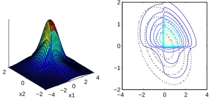
Characteristics related to this last bullet point that are easy to visualize include: • Leptokurtosis - high peak; more variation; higher probability in tails • Platykurtosis - flatter; less variation; lower probability in tails
• Skewness - asymmetric; higher probability in one tail, lower probability in other. Examples can be seen in Figures 1, 2, and 3, generated by the multivariate power exponential distribution given in Section 7.1. In the right pane of all three plots, the heavy black dotted contours are from the Gaussian distribution, for comparison. Characteristics in the first and last figures are most common in real multivariate data. Unfortunately, in the literature the
−4 −2 0 2
4
−2 0 2
x1
x2 −2−4 −2 0 2 4
−4 −2 0 2
4
−2 0 2
x1
x2 −2−4 −2 0 2 4
−1 0 1 2
Figure2: Surfae andontourplotforplatykurtidata(blakontours=Gaussian).
−4 −2 0 2
4
−2 0 2
x1
x2 −2−4 −2 0 2 4
−1 0 1 2
Figure3: Surfae andontourplotforskeweddata (blakontours=Gaussian).
common answer to nonnormality, has been the utilization ofBox-Cox transformationsof[3], which does not seem to work consistently well, in the context of both univariate and multi-variate regression models.
Of course, when performing regression analysis, it is not usually the case that all variables in X have significant predictive power over Y. Choosing an optimal subset model has long been a vexing problem. Typical methods for selecting a subset regression model include:
• Forward stepwise analysis • Backward stepwise analysis
• Partial sums-of-squares and sequential F-tests • consideration of reduced rank regression models.
q = 10. There are 210−1 = 1023 possible nontrivial subsets of the predictors. This is clearly too many models to humanly consider, and yet this is a relatively small problem. Con-sider a dataset we have from a large fractional factorial experiment with q =56; there are 256−1=72, 057, 594, 037, 927, 936 possible subset models. This is far too many for even a computer to automatically evaluate in a timely manner. Little headway has been made in finding the best subset MVR model from a global perspective.
In our results, we demonstrate the value of the genetic algorithm (Section 5), driven by information criteria as a fitness function. We substitute the GA as a computationally feasible and efficient approach for complete combinatorial subset analysis. For the subset regression model, we use the notation X∗ ∈Rn×q∗, where q∗ is the number of variables not excluded
from the model, such thatq∗∈1,q.
3.
I C OM P
: A New Information Measure of Complexity for Model Selection
Perhaps the most basic information criteria is the Kullback-Liebler divergence (KL), first introduced by[24](also called KL distance, or KL information). This information divergence measures the difference between two probability distributions. If we have some data for which we know the true distribution f, we can use the KL divergence to determine whether f1 or f2 more accurately represents the truedata generating process(dgp). f1andf2could be different distributions, or the same distribution as f with different parameters. When a true model is known, as in simulation studies, we can compute the KL divergence for all competing models, with the assumption that the distance for the true model will be the closest to 0.
3.1.
I C OM P
for Correctly Specified Models
Assuming that the model is correctly specified, or the true model is in the model set con-sidered, Akaike[1]introduced his well-known Akaike’s Information Criteria (AI C). Acknowl-edging the fact that any statistical model is merely an approximate representation of the true dgp, information criteria attempt to guide model selection according to Occam’s Razor. One restatement of Occam’s Razor is:
“Of all possible solutions to a problem, the simplest solution is probably the best, ceteris paribus”. This principle of parsimony requires that as model complexity increases, the fit of the model must increase at least as much; otherwise, the additional complexity is not worth the cost. Virtually all information criteria penalize a bad fitting model with negative twice the maxi-mized log likelihood, as an asymptotic estimate of the KL information. The difference, then, is in the penalty for model complexity. The simplest information criteria areAI C andSBC [37], shown below.
In both cases, m is the number of parameters estimated in the model. When using any in-formation criterion to perform model selection, we choose the model corresponding to the lowest score as providing the best balance between good fit and parsimony. It can sometimes be difficult to attach significance (not statistically) to differences in information criteria scores when attempting to select a most appropriate model. To resolve this, we may compute rel-ative weights which can be interpreted as theprobability that a given model is the most appropriate. The weights are computed as in (14),
Wi=
e−I Ci−
min(I C) 2
PL
i=1e−
I Ci−min(I C) 2
, (14)
whereiindexes the Lmodels evaluated.
In contrast to AI C and SBC, I COM P, originally introduced by[4], is a logical extension of AI C and SBC which is based on the structural complexity of an element or set of random vectors via the generalization of the information-based covariance complexity index of[42]. InI COM P, lack-of-fit is still penalized by twice the negative of the maximized log likelihood, while a combination oflack-of-parsimonyandprofusion-of-complexityare simultaneously penalized by a scalar complexity measure, C, of the model covariance matrix. In general, I COM Pis defined by
I COM P=−2 logL( ˆθ| y) +2C(C ovÔ( ˆθ)), (15) where C ovÔ( ˆθ) indicates the estimated model covariance matrix. Each term in (15) approx-imates one KL distance. There are several forms and justifications of I COM P, two of which are detailed here in what follows.
3.1.1. I COM P as an Approximation to the Sum of Two KL Distances
For the following, we need the first order maximal entropic complexity of[4]as a generaliza-tion of the model covariance complexity of[42], given by
C1(C ovÔ( ˆθ)) = s
2log
tr(ÔC ov( ˆθ))
s −
1
2log|C ovÔ( ˆθ)|,s=r ank(ÔC ov( ˆθ)). (16) The greatest simplicity, that is zero complexity, is achieved when the model covariance matrix is proportional to the identity matrix, implying that the parameters are orthogonal and can be estimated with equal precision.
Proposition 1. For a multivariate normal linear or nonlinear structural model we define the general form of I COM P as
Proof. Suppose we consider a general statistical model of the form given by
y=m(θ) +ǫ, (18)
where:
• y= (y1,y2, . . . ,yn)is ann×1 random vector of response values inRn;
• θ is a parameter vector inRk;
• m(θ)is a systematic component of the model in Rn, which depends on the parameter
vectorθ, and its deterministic structure depends on the specific model considered; and • ǫis ann×1 random error vector with
E(ǫ) =0, and E ǫǫ′= Σ(ǫ). (19)
Following[9], we denoteθ∗to be the parameter vector of thetrue operating model, andθ to be any other value of the vector of parameters. Let f(y|θ)denote the joint density function of y givenθ, and let f(y|θ∗)indicate the true model. Further, letK L(θ∗|θ)denote the KL distance between the true model. Then, since yi,i=1, 2, . . . ,nare independent, we have:
K L(θ∗,θ) =
Z
Rn
f(y |θ∗)log
f(y|θ∗)
f(y|θ)
d y
=
n
X
i=1
Z
fi(yi|θ∗)logfi(yi |θ∗)d yi
− n
X
i=1
Z
fi(yi|θ∗)logfi(yi|θ)d yi, (20)
where fi,i=1, 2, . . . ,nare the marginal densities of the yi. Note that the first term in (20) is the usualnegative entropy H(θ∗;θ∗) =H(θ∗), which is constant for a given fi(yi |θ∗). The second term is equal to:
− n
X
i=1
E logfi(yi|θ), (21)
which can beunbiasedly estimatedby −
n
X
i=1
logfi(yi|θ) =−logL(θ | y). (22)
Of course, logL(θ| y)is the log likelihood of the observations evaluated atθ. In practice, we would estimate the parameter vector for a modelM, typically using the MLEθˆM, and so use the maximized log likelihood
− n
X
i=1
logfi(yi |θˆM) =−logL( ˆθM| y). (23)
On the other hand, a model M gives rise to anasymptotic covariance matrix:
C ov( ˆθM) = Σ( ˆθM) (24)
for the MLEθˆM. That is,
ˆ
θM∼N(θ∗,Σ( ˆθM) =F−1). (25) Now invoking the C1(·) (16) complexity on Σ( ˆθM)can be seen as the KL distance between the joint density and the product of marginal densities for a normal random vector with covariance matrix Σ( ˆθM), maximized over all orthonormal transformations of that normal random vector[see 6]. Hence, using the estimated covariance matrix, we defineI COM P as the sum of two Kullback-Liebler distances given by:
I COM P( ˆF−1) = −2 n
X
i=1
logfi(yi|θˆM) +2C1( ˆΣ( ˆθM))
= −2 logL( ˆθM | y) +2C1( ˆF−1). (26)
Some observations:
• The first component ofI COM P( ˆF−1)in (26) measures the lack of fit of the model, and the second component measures the complexity of the estimated IFIM, which gives a scalar measure of the celebratedCramér-Rao lower bound matrix(CRLB), taking into ac-count the accuracy of the estimated parameters and implicitly adjusting for the number of free parameters included in the model.
• It is an intrinsic measure of uncertainty, and, furthermore, it is a quality metric of the estimation procedure. For more on this, and for some immediate physical motivation, we refer the readers to the interesting book by[14]. Also, see,[12]and[32, 33, 34]. • I COM P( ˆF−1) contrasts the trace and the determinant of the IFIM, and this amounts
to a comparison of the geometric and arithmetic means of the eigenvalues of the IFIM, i.e.:
I COM P( ˆF−1)−2 logL( ˆθM| y) +2 log
λa
λg
. (27)
This looks likeCAI C of[5], M D L of[35], and SBC of[37], with the exception that lognis replaced with logλa
λg
.
3.1.2. I COM P as an Estimate of Posterior Expected Utility Following the results from[9], we make the following proposition.
Proposition 2. I COM P as a Bayesian criterion close to maximizing a posterior expected utility (PEU) is given by
Proof. Consider
• Let L(θM| y)be the likelihood function of the parameter vector for a given vector y of observations.
• Let fP r ior(θ |M)denote theprior density functionofθ on the modelM; fPos t(θ | y)is the correspondingposterior density.
• LetF(θM)denote the Fisher information matrix for the nobservations corresponding to modelM, and letmbe the dimension ofM.
Following[30], we consider the KL distance between the posterior and the prior densities for modelM given by
K L(fPos t(θ| y),fP r ior(θ |M)) =
Z
ΘM
fPos t(θ| y)logfPos t(θ| y)dθ−
Z
ΘM
fPos t(θ | y)logfP r ior(θ |M)dθ
=H(fPos t(θ| y))−
Z
ΘM
fPos t(θ| y)logfP r ior(θ|M)dθ. (29)
Further following Poskitt’s arguments, under regularity conditions which guarantee the asymp-totic normality of the posterior distribution, that is, when
fPos t(θ| y)∼=N( ˆθ,Σ( ˆθ) = ˆF−1), (30) it can be shown that
K L(fPos t(θ| y),fP r ior(θ|M)) =−m
2 log(2π)− m
2 − 1 2log|Fˆ
−1| −logf
P r ior(θ|M). (31) One can argue, as did Poskitt, that a utility U1 can be defined as logU1 = the KL distance given by (31). In Bayesian design of experiments, following the suggestion of [25], several authors have considered the Kullback-Liebler divergence as a utility function. For more on this, see[10]. In our case, we propose to multiply the utilityU1by a utility U2 equal to
U2=exp−a×C1( ˆF−1). (32) If we havea=1, our utility isU=U1×U2, and the log of that utility equals:
log(U) =−m
2 log(2π)− m
2 − 1 2log|Fˆ
−1| −logf
arithmetic means of the eigenvalues ofIFIMalready shown in (27).
If we apply Poskitt’s Corollary 2.2 (maximizing posterior expected utility), or theLaplace expansionresults of[21], it follows that, under some regularity conditions, if the parameter vectorθ lies in modelM, the posterior expected utility can be approximated by
log(P EU)∼=logf(y|θˆM) + m
2 log(2π) + 1 2log|Fˆ
−1|+log(U) +logf
P r ior( ˆθM|M), (34) up to order O(1
n) and up to some terms which do not depend on the model M. Replacing log(U)in this equation by its value in (33), some terms cancel out. We thus obtain a criterion, to be maximized to choose a model:
logf(y|θˆM)− m
2 −C1( ˆF
−1) +logf(M), (35)
but maximizing this is equivalent to minimizingI COM PP E U( ˆF−1), given by
I COM PP E U( ˆF−1) =−2 logL( ˆθM| y) +m+2C1( ˆF−1) +logf(M). (36) Finally, assuming that f(M)is constant for all models in (36), we have
I COM PP E U( ˆF−1) =−2 logL( ˆθM| y) +m+2C1( ˆF−1). (37)
Note that when we defined the utility U2=exp
−a×C1( ˆF−1)
, (38)
we considered the constant multiplier a to be 1 in obtaining the result shown above. In-deed other choices of a are possible and equally justifiable, giving rise to different penalty functionals. For example, a choice ofa=lognwould yield
I COM PP E U_L N( ˆF−1) =−2 logL( ˆθM | y) +m+log(n)C1( ˆF−1), (39) which clearly enforces a stricter penalty. One can choose yet other forms of the utilityU2 and its exponent to obtain several consistent forms of I COM P, which are justifiable, to penalize overparametrization of the models under consideration. For more on I COM P we refer the readers to[8].
3.2.
I C OM P
for Misspecified Models
to check misspecification of a model. We define the Hessian form of the Fisher information matrix as
F =−E
∂2logL(θ) ∂ θ ∂ θ′
(40)
and the outer-product form as
R=E
∂logL(θ) ∂ θ ·
∂logL(θ) ∂ θ′
, (41)
where the expectations are taken with respect to the true but unknown distribution. Following
[13],[17, page 237],[18, page 270],[19, page 391],[45], and others, suppose that the fitted model is incorrectly specified. Letg(y|θ∗)be the true model. Without knowing, suppose we fit f(y |θ) to a random sample y1, . . . ,yn ofnobservations. Under mild conditions, the log likelihood of the fitted model
logL(θ) =
n
X
i=1
logf(yi|θ) (42)
is maximized at the MLEθˆ, and asn−→ ∞the average maximized log likelihood function
logL( ˆθ| y) = 1
n n
X
i=1
logf(yi |θ)ˆ −→
Z
f(y|θg∗)logg(y)d y, (43)
whereθ∗gis the value ofθ that minimizes the KL information
K L=
Z
log
g(y |θ∗)
f(y|θ)
g(y|θ∗)d y, (44)
with respect toθ. Thusθg∗is the “least bad” value ofθ given the misspecified model. Taking the partial derivative of (43) w.r.tθ, we have
0=
Z
∂logf(y|θ)
∂ θ g(y)d y, (45)
withθˆobtained from the finite-sample version of the previous equation given by
0= 1
n n
X
i=1
∂ logf(yi |θ)ˆ
∂ θ . (46)
Now expansion of this aboutθg∗yields
ˆ
θ=. θg∗+
−1
n n
X
i=1
∂2logf(yi|θg∗) ∂ θ ∂ θ′
−1
1
n n
X
i=1
∂logf(yi|θg∗) ∂ θ
Which provides us with 1
n n
X
i=1
∂2logf(yi|θg∗)
∂ θ ∂ θ′
p −→
(
E ∂
2logf(y|θ∗ g)
∂ θ ∂ θ′
!)
=−F(θg∗), (48)
the inner-product form of the FIM, and 1
n n
X
i=1
∂ logf(yi |θg∗)
∂ θ
p −→
¨
E
∂logf(y|θ∗ g)
∂ θ
·
∂logf(y |θ∗ g)
∂ θ
«
=R(θg∗) (49)
the outer-product form of the FIM. These two forms are useful to check for model misspecifi-cation. This gives us the following result, with the derivation in the appendix.
Theorem 1. Based on an iid sample, y1, . . . ,yn, and assuming regularity conditions of the log likelihood function hold, we have
ˆ
θ ∼N(θ∗g,F−1RF−1), orpn( ˆθ−θg∗)∼N(0,F−1RF−1). (50) Note that this tells us explicitly
C ov(θg∗)M isspec=F−1RF−1, (51) which is called thesandwichor robustcovariance matrix, since it is a correct variance matrix whether or not the assumed or fitted model is correct. Of course, in practice the true model and parameters are unknown, so we estimate this with
Ô
C ov( ˆθ) = ˆF−1RˆFˆ−1. (52) If the model is correct, we must haveFˆ−1Rˆ=I, so
Ô
C ov( ˆθ) = ˆF−1RˆFˆ−1=IFˆ−1= ˆF−1.
Thus, in the case of a correctly specified model,C ovÔ( ˆθ) = ˆF−1. However, when the model is misspecified, this is not the case. Under misspecification, several forms of I COM Ppreviously defined are given as follows.
I COM P(ÔC ov( ˆθ))M I SP=−2 logL( ˆθ| y) +2C1( ˆF−1RˆFˆ−1). (53) I COM P(C ovÔ( ˆθ))M I SP_P E U =−2 logL( ˆθ| y) +tr( ˆF−1Rˆ) +2C1( ˆF−1RˆFˆ−1). (54) I COM P(C ovÔ( ˆθ))M I SP_P E U_L N=−2 logL( ˆθ | y) +tr( ˆF−1Rˆ) +log(n)C1( ˆF−1RˆFˆ−1). (55) In the next section, we will see howmgot transformed into tr( ˆF−1Rˆ)in the latter two. Result 1. If
I COM P6=I COM PM I SP
we say the model is misspecified, or equivalently
3.3. Bias of the Penalty
When we assume that the true distribution does not belong to the specified parametric family of pdfs, that is, if the parameter vectorθof the distribution is unknown and is estimated by maximizing the likelihood, then it is not any longer true that the average of the maximized log likelihood converges to the expected value of the parameterized log likelihood. That is,
1
nlogL( ˆθ| y) = 1 n
n
X
i=1
logf(yi |θ)ˆ 9Eylogf(y |θ)ˆ . (56)
In this case, the asymptotic bias, b, between these two terms is given by
b=EG 1 n
n
X
i=1
logf(yi |θ)ˆ −
Z
R
logf(y |θˆ)d G(y)
!
= 1
ntr(F
−1R) +O(n−2), (57)
where the expectation is taken over the true distributionG =Qni=1G(yi)[22]. We note that tr(F−1R)is the well knownLagrange-multiplier test statistic. See, for example,[40, 20, 38]. Since we typically have MLE’s and not true parameter values, we have to estimate the bias using
bb= 1
ntr( ˆF
−1Rˆ). (58)
Thus, we have: Generalized Akaike’s information criterion,GAI C, defined by
GAI C = −2 n
X
i=1
logf(yi|θ) +ˆ 2 tr( ˆF−1Rˆ)
= −2 logL( ˆθ| y) +2 tr( ˆF−1Rˆ). (59) In the literature of model selection,GAI C is also known as Takeuchi’s[40]information crite-rion (T I C), orAI CT.
When the model is correctly specified the asymptotic bias reduces to:
b = 1
ntr(F
−1R) +O(n−2)
= 1
ntr(Im) +O(n −2)
= 1
nm+O(n −2),
which givesAI C as a special case ofGAI C given by
AI C=−2 logL( ˆθ| y) +2m,
criteria is possible, and their asymptotic properties are well explained in[23, p. 176]. When the true model is not in the model set considered, which is often the case in practice,AI C will have difficulties identifying the best fitting model, as it does not penalize the presence of skewnessandkurtosis.
We do not claim that the I COM P criterion derived in this paper captures all forms of model misspecification. We only pay attention to the case where the probabilistic distribu-tional form of the fitted model departs from normality within the multivariate regression framework.
In reviewing the literature, we note that Sawa’s [see 36] BI C (should not be confused with SBC which is also sometimes referred to as BI C) also adjusts penalization according to misspecification, but there is no relationship between I COM P and BI C, except perhaps that the underlying formulation of the two criteria are both based on the KL information. Sawa’s penalty term is not an entropic function of the complexity of the estimated sandwich covariance matrix of the model. As shown above, the I COM P criterion can be seen as an approximation to the sum of two KL distances. Similarly, I COM P is not necessarily related to Wei’s[see 43, page 30]Fisher Information Criterion (F I C) in the standard multiple re-gression model. InF I C, the incorporation of the determinant of the Fisher information is not based on any theoretical grounds such as the entropic complexity measure of the covariance matrix inI COM P. F I C is more related to thePredictive Least Squares(PLS) criterion, as[43]
demonstrates.
4. Information Complexity for the Multivariate Regression Models
4.1.
I C OM P
and Information Criteria for Correctly Specified MVR Models
For multivariate regression, the number of estimated parameters ism=pq+p(p+1)/2; we have a coefficient for each of theqcovariates for each of the presponses, and allow for a fully general covariance matrix, which has p(p+1)/2 unique elements. Thus, theAI C-type criteria are given as
AI C=nplog(2π) +nlog|Σˆ|+np+2(pq+ p(p+1)
2 ), and (60)
SBC =nplog(2π) +nlog|Σˆ|+np+log(n)(pq+ p(p+1)
2 ). (61)
The typicalI COM P( ˆF−1)is
I COM P( ˆF−1) =nplog(2π) +nlog|Σˆ|+np+2C1( ˆF−1). (62) Rather than compute and store the entire IFIM, we can computeC1( ˆF−1) after “opening it up” as shown in (63):
+ slog(1
s
tr( ˆΣ)tr[(X′X)−1] + 1
2n(tr( ˆΣ
2) +tr( ˆΣ)2+2
p
X
j=1 (σ2j j)2)
)
− (p+q)log|Σˆ|+plog|X′X|+ p(p+1)
2 log(n)−plog(2), (63) where(σ2
j j)2indicates the square of the jthdiagonal element ofΣˆ. To computeI COM P( ˆF−1)P E U, one would simply add m to (63). For I COM P( ˆF−1)P E U_L N, multiply the I COM P( ˆF−1)
penalty by log(n)/2, then addm.
4.2.
I C OM P
for Misspecified MVR Models
Model misspecification is an important issue with regression models. To protect the re-searcher against model misspecification, we needC ovÔ( ˆθ) = ˆF−1RˆFˆ−1. Fˆ−1 is repeated in (64)
ˆ
F−1=
ˆ
Σ⊗(X′X)−1 0
0′ 2nD+p( ˆΣ⊗Σ)ˆ D+p′
, (64)
ˆ
Ris derived in the appendix, and we show the results here.
ˆ
R=
Σˆ−
1⊗X′X 1
2( ˆΣ
−1/2⊗X′)ˆΓ
1D+p ′∆ 1/2∆D+pΓˆ1′( ˆΣ−12⊗X) 1
4∆D
+
pΓˆ∗2D
+
p ′∆
(65)
This matrix takes into consideration the actual sample skewness
ˆ
Γ1=vecZvec(Z′Z−nIp)
′
, (66)
and kurtosis
ˆ
Γ∗2= (vecZ′Z)(vecZ′Z)′+n2(vecIp)(vecIp)′. (67) We define
∆ =D′p( ˆΣ−1/2⊗Σˆ−1/2)Dp, and we standardize the response matrix with
Z= (Y−Xβ) ˆˆ Σ−1/2.
The vec(·)operator stacks the columns of a matrix on top of each other, such that Z∈Rn×p−→vecZ∈Rnp×1,
andΣˆ−1/2indicates the inverse of the matrix square root defined by
ˆ
Σ1/2Σˆ1/2= ˆΣ. In cases where the model is correctly specified, we have
Γ1reduces to0, andΓ∗2−→2nDpD+p, such thatRˆ= ˆF, in theory.
Thus, the misspecification-resistant estimator of the model covariance matrix is given in (69)
Ô
C ov( ˆθ) = Fˆ−1RˆFˆ−1 =
ˆ
Σ⊗(X′X)−1 1
n( ˆΣ
1/2⊗(X′X)−1X′)ˆΓ
1Dp∆−1
1
n∆−
1D′ pΓˆ′1( ˆΣ
1/2⊗X(X′X)−1) 1
n2∆−1D′pΓˆ∗2Dp∆−1
. (69)
A procedure for “opening up” ÔC ov( ˆθ)is shown in Appendix 2. As with the regularI COM P, this procedure simplifies the computation, since the entire covariance matrix does not have to be built and stored.
There is an issue of matrix stability to be addressed with the sandwich covariance ma-trix, however. In both simulated and real datasets, we have observed that the matrix is consistently rank-deficient. We performed simulation studies similar to those detailed in Sec-tion 7.2, in which the model was correctly specified, and observed thatI COM PM I SP(C ovÔ( ˆθ))
andI COM P( ˆF−1)did not, in fact, select similar models. It appears that numerical issues with the sandwich covariance matrix prevent it from approximating the IFIM when the model is correctly specified. As an example, consider a dataset in whichp=2 andq∗=8. The number of parameters estimated ism=19, and the model covariance matrix is of size 19×19. How-ever, the rank is only 16. Of course, the determinant is 0. We employ the robust covariance estimators (discussed in Section 6) to ensureC ovÔ( ˆθ)is of full rank.
4.3. KL Information between True and Fitted Model
Suppose that we denote a true multivariate regression model by
Mt:Y =X∗B∗+E∗,C ov(vecY∗) = Σ∗⊗In (70) and the fitted (or candidate) multivariate regression model by
Mf :Y =X B+E,C ov(vecY) = Σ⊗In. (71) Under the multivariate normal assumption, the log likelihood of the true modelMtis
logL(Mt) =−np
2 log(2π)− n 2log|Σ
∗| −1
2tr[(Y−X
∗B∗)Σ∗−1(Y−X∗B∗)′]. (72)
The log likelihood of the fitted modelMf is
logL(Mf) =− np
2 log(2π)− n
2log|Σ| − 1
2tr[(Y −X B)Σ
−1(Y−X B)′]. (73)
Then the log likelihood of the difference between the true model and the fitted model becomes
=log
|Σ|
|Σ∗|
+1
ntr[(Y−X B)Σ
−1(Y−X B)′]−1
ntr[(Y−X
∗B∗)Σ∗−1(Y −X∗B∗)′]. (74)
Now, taking the expectation with respect to the true model, we obtain the Kullback-Leibler distance as[5]:
K L = E∆logL(Mt,Mf)
= log
|Σ|
|Σ∗|
+tr(Σ−1Σ∗) +1
ntr[(X
∗B∗−X B)Σ−1(X∗B∗−X B)′]−p. (75)
Using the maximum likelihood estimators
ˆ
B= (X′X)−1X′Y, andΣ =ˆ (Y−X ˆ
B)′(Y−XBˆ)
n =
Y′M Y
n , (76)
we have the estimated KL
Ó
K L=log
|Σˆ|
|Σ∗|
+tr( ˆΣ−1Σ∗) +tr[ ˆΣ−1(X∗B∗−XBˆ)(X∗B∗−XBˆ)′]−p. (77)
This gives us a yardstick in comparing the performance of model selection criteria between the true and the fitted model in how close they are to the KL distance, especially in simulation protocols, since the true model is known by design. By means of simulation study, we can investigate the finite sample behavior of I COM P criteria both when the model is correctly specified, and the model is misspecified.
5. Genetic Algorithm (GA)
The GA is a search algorithm that borrows concepts from biological evolution. Biological chromosomes, which determine so much about organisms, are represented as binary words – these determine the composition of possible solutions to an optimization problem. Unlike most search algorithms, the GA simulates a large population of potential solutions. These solutions are allowed to interact over time; random mutations and natural selection allow the population to improve, eventually iterating to an optimal solution. For multivariate regression subsetting, each chromosome is aq-length vector such that each locus represents the presence (1) or absence (0) of a specific predictor. An example chromosome may be[10011001]; in this case, predictors 1,4,5,8 will be used for OLS while 2,3,6,7 will not. The general procedure in the GA is simple and straightforward:
1. Generate initial population of chromosomes 2. Score all members of current population
3. Determine how current population is mated and represented in next generation 4. Perform chromosomal crossover and genetic mutation
5. Pass on offspring to new generation
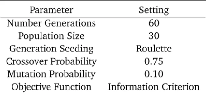
As seen in Table 1, there are 8 major parameters used to define the operation of the genetic algorithm. These are all discussed, along with implementation methods, below.
Table1: SampleGenetiAlgorithmparameters.
Parameter Setting
Number Generations 60
Population Size 30
Generation Seeding Roulette Crossover Probability 0.75
Mutation Probability 0.10
Objective Function Information Criterion
5.1. Number Generations
Each iteration in the GA is called a generation, for obvious reasons. Thus, this parameter is fairly self explanatory. There is an important trade-off to note, when selecting the number of generations through which the GA will run. More generations mean more computation time; however, not allowing the process to go through enough iterations can mean termination with a suboptimal result.
5.2. Population Size
This parameter,P, determines the number of chromosomes are considered in each genera-tion. In general, one would expect convergence times to decrease as population size increases, up to a point. After that point, the computational time (and hence, time to convergence) increases quickly. In other unpublished research, performance of the GA when used for mul-tivariate subsetting was analyzed as operational parameters were purposely varied. In this case, the goal was to maximize the frequency, across all generations, with which the proce-dure selected the optimal subset. Tests were performed on a dataset for which the optimal subset was known. It was determined that the GA was robust to all parameters tested (not all parameters used here were varied) excepting population size; though in this case, variation in population size only explained half the variation in the response.
5.3. Generation Seeding
Figure4: Coneptualroulettewheel.
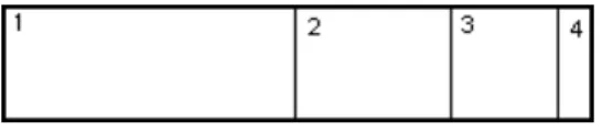
sum of these bins is computed. As an example, consider the sorted list of 4 chromosomes -the bin widths are given as bi=0.40 0.30 0.20 0.10, so the bin limits are
bin 1 2 3 4
Lower Limit 0.00 0.40 0.70 0.90 Upper Limit 0.40 0.70 0.90 1.00
.
Clearly, the larger bins are at the beginning, corresponding to the most fit chromosomes. At this point, P random numbers are generated uniformly from[0, 1]and placed in the appro-priate bin. For each random variate in bin i, chromosome i gets represented in the next generation. In this way, chromosomes with a better objective function value are overrepre-sented in the mating pool. The last step, then, is to randomly permute the ordering of the chromosomes before mating; after permutation, mating occurs just as in the sorted method.
5.4. Crossover Probability
There are several ways in which crossover can be implemented, including: • Single-point (fixed or random)
• Multiple-point (fixed or random) • Uniform (fixed or random)
We’ve chosen to use the simplest - randomized single-point crossover. For each mating pair, a random uniform variate is selected from integers in the range2,q−1, this range is used, rather than 1,q, to protect against endpoint crossovers. For a given pair of mating chro-mosomes, their right-most portions are traded starting from this point. For example, if the crossover point is 2, we have
1 11 0 0 1 01 0 1
−→
1 1 0 1 01 0 1 0 1
.
For each mating pair, a random variate fromU(0, 1)is generated; if it is less than the crossover probability, the mating pair undergo the crossover operation. Otherwise, the offspring are pure genetic replicants of the parents.
5.5. Mutation Probability
5.6. Objective Function
More or less, all optimization or search procedures need some objective function to either maximize or minimize. There is a large universe of appropriate functions that could fill this role. For this problem we’ve chosen to use a class of criteria called information criteria. Specifically, we present the use of Bozdogan’sI COM P which drives effective model selection in the face of model misspecification.
6. Robust Covariance Estimation
In many real-life problems, covariance matrices can become ill-conditioned, non-positive definite, or even singular. This is especially true in cases of regression with highly collinear predictors. It is also seen in situations in which there are not many more observations than there are measurements, or variables - i.e., when it is not the case that n ≫ p. The usual response to singular or ill-conditioned covariance matrix estimates is ridge regularization,
ˆ
Σ∗=Σ +ˆ αIp, (78)
which works to counteract the ill-conditionedness by adjusting the eigenvalues ofΣˆ. Usually, the ridge parameter,α, is chosen to be very small. This, of course, begs the questions
• "How large shouldαbe?" • "How small canαbe?".
The answer to these questions is to use robust covariance estimators. Many different robust, or smoothed, covariance estimators have been developed as a way to data-adaptively improve ill-conditioned and/or singular covariance matrix estimates. Several of them work by the same mechanism as ridge regularization - perturb the diagonals, and hence, the eigenval-ues. Although we use only the MLE/EB covariance estimator in our reported results, several methods implemented in our algorithm include:
• Maximum Likelihood/Empirical Bayes
ˆ
ΣM L E/E B= ˆΣ + p−1
(n)tr( ˆΣ)Ip (79)
• Stipulated Ridge,[39] ˆ
ΣSRE = ˆΣ +p(p−1)(2n)tr( ˆΣ)−1Ip (80) • Stipulated Diagonal,[39]
ˆ
ΣSDE= (1−π) ˆΣ +πd ia g( ˆΣ), π=p(p−1)2n(tr( ˆΣ−1)−p)−1 (81) • Convex Sum,[31, 11]
ˆ ΣC SE=
n
n+mΣ + (ˆ 1− n n+m)
tr( ˆΣ)
p
Ip (82)
0<m< 2
p(1+β)−2 p−β , β=
• Thomaz Stabilization[41]
ˆ
ΣT homaz=VΛ∗V (83)
Λ∗=
max(λ1,λ) 0
max(λ2,λ)
... ...
0 max(λp,λ)
(84)
λi=itheigenvalue,λ=mean eigenvalue,V =matrix of eigenvectors
When a small amount of perturbation is all that is required,ΣˆM L E/E Bhas a certain appeal. As is clear in (79), this is the same form of the naive ridge regularization, whereαis determined by the data.
For the results reported here, we used the Empirical Bayes estimator, so as to perturb the estimates as little as possible. Even then, we prefer to not change the problem more than necessary, so we perform two tests for matrix condition:
1. Is the reciprocal of the condition number small:κ−1( ˆΣ)≤1e−10? 2. Is the MLE nonpositive definite?
If the answer to either question is in the affirmative, we apply the robust covariance estimator to give us a well-conditioned estimate,Σˆ∗.
7. Numerical Results
7.1. Simulation with Correlated Redundant Variables
We first demonstrate the performance of misspecification-robust information criteria on a simulated dataset using a complex simulation protocol. We begin by generating five correlated regressors, with x4 andx5 redundant.
x0 = 1 (constant) x1 = 10+ǫ1
x2 = 10+ρǫ1+αǫ2
x3 = 10+ρǫ1+0.5604αǫ2+0.8282αǫ3 x4 = −8+x1+0.5x2+ρx3+0.5ǫ4 x5 = −5+0.5x1+x2+0.5ǫ5
Theǫi are drawn from a standardized Gaussian distribution,ρ=0.3 controls the correlation, as doesα=p1−ρ2. Thus far, we haveX =x
0,x1,x2,x3,x4,x5
. We now turn our focus to the response matrix, which we create as:
B =
−8 −5 1.0 0.5 0.5 0.0 0.3 0.3 .
To make this a truly misspecified model, we generate the error terms from the multivariate power exponential distribution (MPE). From[16], the density function for the MPE is shown in (85).
f(xi|µ,Σ,β) = pΓ(
p
2)|Σ|
−1 2
2πp2Γ(1+ p
2β)2 1+p
2β
exp(−1
2
(xi−µ)Σ−1(xi−µ)′β) (85)
This distribution includes others as special cases: • Whenβ=1, we have themultivariate Gaussian • Whenβ=1/2, we have themultivariate Laplace • Whenβ→ ∞, we have themultivariate uniform We generate the error terms two different ways:
S1:µ= [0, 0],Σ =
1 0.5 0.5 1
,β=0.75 S2:µ= [0, 0],Σ =
1 0 0 1
,λ= [2,−2]
In simulation S2, the error terms matrix is created as two independent columns of skewed univariate power exponential distributions, with one skewed right and the other being left-skewed. The skewness is imparted utilizing Azzalini-type skew, with the functional form shown in (86) - see[2]. Figure 5 shows two examples.
g(x) =2f(x)F(λx)∼Skew(f,λ) (86)
−200 −10 0 10 0.05 0.1 0.15 0.2 0.25 0.3
ε1,λ = 2
−5 0 5 10 15 0 0.05 0.1 0.15 0.2 0.25 0.3
ε2,λ = −2
Figure5: DemonstratingtheunivariateAzzalini-typeskewedPE.
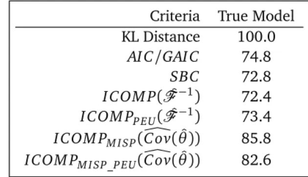
re-Table2: Abbreviated%modelhitsoutofM=500simulationsofS1withn=500.
Criteria True Model KL Distance 100.0
AI C/GAI C 74.8
SBC 72.8
I COM P( ˆF−1) 72.4 I COM PP E U( ˆF−1) 73.4 I COM PM I SP(C ovÔ( ˆθ)) 85.8 I COM PM I SP_P E U(C ovÔ( ˆθ)) 82.6
Table3: %modelhitsoutof M=500simulationsofS1withn=1000.
Subset AI C/GAI C SBC I COM P( ˆF−1)/P EU I COM PM I SP(C ovÔ( ˆθ))/P EU
{0, 1, 2, 3, 4, 5} 1.6 0.0 0.0/0.0 0.0/0.0
{1, 2, 3, 4, 5} 0.0 0.0 0.4/0.2 0.0/0.0
{0, 1, 3, 4, 5} 0.2 0.0 0.0/0.0 0.0/0.0
{0, 1, 2, 3, 5} 11.0 0.2 1.2/0.4 2.0/0.8
{0, 1, 2, 3, 4} 12.2 0.0 0.0/0.0 1.2/0.8
{0, 1, 3, 5} 0.0 0.4 0.2/0.2 0.4/0.4
{0,1,2,3} 75.0 98.2 98.2/99.2 96.2/97.6
{0, 1, 2} 0.0 1.2 0.0/0.0 0.2/0.4
sults from the experiment withn=500 observations generated from the simulation protocol. There are, of course, 26−1=63 possible subsets of the covariates; not counting subsets never selected, there were too many to show in detail here. As such, we’re reporting the percent of simulations in which the criteria selected exactly the true model X∗=x0,x1,x2,x3. It is interesting to note thatAI C and GAI C performed identically. We also see thatAI C seems more appropriate for smaller samples. I COM PM I SP(C ovÔ( ˆθ))performed well, only selecting a model that did not include the true model in 11% trials. The misspecified I COM Pshit the true model with the highest frequency of all the criteria.
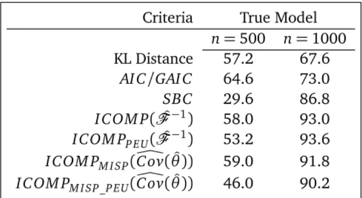
Table4: Abbreviated%modelhitsoutofM=500simulationsofS2.
Criteria True Model n=500 n=1000 KL Distance 57.2 67.6
AI C/GAI C 64.6 73.0
SBC 29.6 86.8
I COM P( ˆF−1) 58.0 93.0 I COM PP E U( ˆF−1) 53.2 93.6 I COM PM I SP(C ovÔ( ˆθ)) 59.0 91.8 I COM PM I SP_P E U(C ovÔ( ˆθ)) 46.0 90.2
Next, we performed to sets of simulation experiments with the S2 model for n=500 and n= 1000. In the presence of asymmetry there was a lot more confusion, with 38 different models being selected by different criteria. Table 4 summarizes the results.
In the presence of skewness, AI C and GAI C performed admirably in the tests with the smaller sample size, whileSBC did not. The I COM Pcriteria performed very well, especially with the larger sample sizes. I COM PM I SP(ÔC ov( ˆθ))proved better than even the KL distance at both selecting the true model, and a model that included the truth. The KL distance per-formed much worse than it did when the errors were generated symmetrically. We also note that, like the S1 simulation, I COM P( ˆF−1)is robust against a high degree of skewness, with performance similar to the misspecified form ofI COM P.
In summary, we observe that in all experiments, AI C and GAI C performed identically. This suggests that considering just estimated bias does not provide much benefit. Effectively adjusting for model misspecification seems to require the entire sandwich covariance matrix.
7.2. Simulation with Redundant and Unnecessary Variables
This simulation protocol, with the multicollinearity and non-Gaussian errors, is a decent test of the performance of information criteria in the presence of misspecification, but we can do better. Thus, we add 15 unrelated variables to our matrix of regressors, such that
X∈Rn×21=x0,x1,x2,x3,x4,x5,
xi ∼U(0,i)|i=6 . . . 20 .
Under this extended simulation protocol, we have 221−1 = 2, 097, 151 different possible models to evaluate, and the true model is still X∗ = x0,x1,x2,x3
. This is a very difficult problem for any criteria to perform well under. We use the genetic algorithm to search the subset space with the settings: population size = 30, number generations= 60, crossover rate= 0.75, mutation rate = 0.10. The four Monte Carlo simulation experiments from the previous section, all withM =100, were performed.
Table5: ModelseletionstatistisfromextendedS1simulations.
Criteria n Model Selected True Model Avg Length
KL Distance 500 {0, 1, 2, 3} 86.0 4
1000 {0, 1, 2, 3} 92.0 4
AIC 500 {0, 1, 2, 3, 6, 10, 12, 19} 6.0 7 1000 {0, 1, 2, 3, 6, 12, 14, 15} 4.0 6
SBC 500 {0, 1, 2} 54.0 4
1000 {0, 1, 2, 3} 94.0 4
GAIC 500 {0, 1, 2, 3, 5, 16, 17} 7.0 7
1000 {0, 1, 2, 3, 15} 4.0 6
I COM P 500 {1, 2, 3, 4} 11.0 7
1000 {1−8, 10, 14, 17, 18} 63.0 5
I COM PP E U 500 {1, 4, 5} 20.0 5
1000 {0, 1, 2, 3} 70.0 5
I COM PM I SP 500 {0, 1, 2, 3} 77.0 4
1000 {0, 1, 2, 3} 89.0 4
I COM PM I SP_P E U 500 {0, 1, 2, 3} 75.0 4
1000 {0, 1, 2, 3} 93.0 4
perfect track record - at best selecting the true model in 92% of the trials. With more infor-mation in the tails, the misspecifiedI COM P criteria performed well regardless of the sample size. In fact, minimization of both criteria across all simulations selectedX∗=x0,x1,x2,x3 as the best model The PEU version did very well, hitting the true model in 93 of the 100 sim-ulations for the larger sample size. Over all simsim-ulations, these two criteria andSBC selected models, on average, with 4 regressors - there was no substantial tendency to overfit. Once again, though, we see the inconsistent behavior ofSBC, only doing really well with the large sample. BothAI C and GAI C performed extremely poorly, both tending to pick models with 2 or 3 extra predictor variables. To their credit, they also displayed a strong tendency to pick models that included the true model (eg. x∗ =x0,x1,x2,x3,x4,x5). The final model se-lected byI COM P( ˆF−1)for the large sample simulation is truly bizarre - 12 regressors, while the average model length was a respectable 5. This seems like it may have been a vagary of simulation. In Table 6, we see the results from one of the many simulations in which the
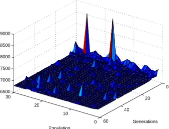
Table6: SummaryfromonesimulationoftheextendedS1protool.
Subset I COM PM I SP(C ovÔ( ˆθ)) Weights # Generations
{0,1,2,3} 6789.73 0.948 30
{0, 1, 2, 3, 5} 6796.30 0.035 25
{0, 1, 2, 3, 5, 14} 6797.80 0.017 1
0 10
20 30
0
20
40
60 6500
7000 7500 8000 8500 9000
Generations 3−dimensional Surface Plot of ICOMP_IFIM_MISP scores.
Population
Figure6: 3-dSurfaeplotofI COM P
M ISP(ÔC ov( ˆθ).
misspecified version of I COM P selectedX∗as the best model. Here we see that the criteria was almost 95% certain that its solution was the true model. Finally, we see, in Figure 6, how much the GA smoothed the search surface, with relatively rare spikes in the I COM P scores. Though this plot doesn’t show it, the simulation found it’s final solution in the 30thgeneration.
Secondly, we performed 100 simulations withn=500 and 100 simulations withn=1000 from the extended protocol with the skewed error terms. Results from these simulations can be seen in Table 7. It seems noteworthy that the KL distance, assuming normality, did not perform substantially better with the increase in sample size. With the smaller sample size, I COM PM I SP(ÔC ov( ˆθ)) did the best job of hitting the true model, at 42%; minimizing both SBC andI COM PM I SP_P E U(C ovÔ( ˆθ))selected the true model. However, when the sample size was increased ton =1000, both misspecified forms of I COM P had the highest hit rates of 80% and 73%, besting the 58% obtained by the KL distance. The only criteria which selected, via minimization, the true model were three of the fourI COM Ps.
Table7: ModelseletionstatistisfromsimulationsofextendedS2.
Criteria n Model Selected True Model Avg Length
KL Distance 500 {0, 1, 2, 3} 48.0 4
1000 {0, 1, 2, 3} 58.0 4
AIC 500 {0, 1, 2, 3, 6, 8} 6.0 6
1000 {0, 1, 2, 3, 14, 16} 8.0 6
SBC 500 {0, 1, 2, 3} 17.0 2
1000 {0, 1, 3, 5} 63.0 4
GAIC 500 {0, 1, 2, 3, 4, 12, 19} 5.0 6 1000 {0, 1, 2, 3, 5, 14, 15} 3.0 6 I COM P 500 {1, 3, 4, 5, 6, 9} 6.0 6
1000 {0, 1, 2, 3, 5} 47.0 5
I COM PP E U 500 {1, 3, 4, 5, 9, 13, 14} 9.0 4
1000 {0, 1, 2, 3} 49.0 5
I COM PM I SP 500 {0, 1, 3} 42.0 4
1000 {0, 1, 2, 3} 80.0 5
I COM PM I SP_P E U 500 {0, 1, 2, 3} 38.0 3
1000 {0, 1, 2, 3} 73.0 4
7.3. GA Performance under Simulations
Table8: Timingtestresults.
q P Possible Models Models Evaluated
per Simulation Average Time
20 30 1, 048, 575 ≤1, 800 1.89s
25 35 33, 554, 431 ≤2, 100 1.82s
35 45 34, 359, 738, 367 ≤2, 700 2.34s
50 60 1, 125, 899, 906, 842, 623 ≤3, 600 2.89s
75 85 3.7779e22 ≤5, 100 4.84s
100 110 1.2677e30 ≤6, 600 7.99s
GHz processor and 2 GB of RAMwhile many other processes were running.
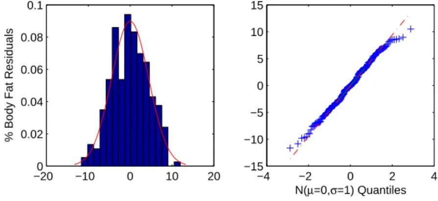
7.4. Real Data - Body Fat Measurement
The first real dataset to be analyzed was the familiar body fat dataset This data is com-posed of body measurement observations fromn=252 men. There are p=2 responses and q= 13 regressors, listed in Table 9. Where not specified, measurements are in centimeters. Accurately measuring body composition, and specifically the percentage that is fat, is an in-convenient and costly procedure. A method for accurately computing these amounts from simple body measurements without requiring underwater weighing is highly desirable.
Table9: Bodyfatdatasetvariables.
y1=Body Density (gm/cm3) y2=Percent body fat from Siri’s equation x0=Constant x7=Hip circumference
x1=Age (yrs) x8=Thigh circumference x2=Weight (lbs) x9=Knee circumference x3=Height (in) x10=Ankle circumference
x4=Neck circumference x11=Extended biceps circumference x5=Chest circumference x12=Forearm circumference
x6=Abdomen 2 circumference x13=Wrist circumference
We first ran the genetic algorithm with population size = 20, using the I COM P( ˆF−1)