Data Mining-Assisted Parameter Tuning of a Search Algorithm

Data Mining-Assisted Parameter Tuning of a Search Algorithm

Jurij Šilc

Computer Systems Department, Jožef Stefan Institute, Jamova cesta 39, SI-1000 Ljubljana, Slovenia E-mail: [email protected]

Katerina Taškova

Institute of Computer Science, Johannes Gutenberg University Mainz, Staudingerweg 9 55128 Mainz, Germany

E-mail: [email protected]

Peter Korošec

Computer Systems Department, Jožef Stefan Institute, Jamova cesta 39, SI-1000 Ljubljana, Slovenia, and Faculty of Mathematics, Science and Information Technologies, University of Primorska

Glagoljaška 8, SI-6000 Koper, Slovenia E-mail: [email protected]

Keywords: data mining, differential ant-stigmergy algorithm, low-discrepancy sequences, meta-heuristic optimization, parameter tuning

Received:December 1, 2014

The main purpose of this paper is to show a data mining-based approach to tackle the problem of tuning the performance of a meta-heuristic search algorithm with respect to its parameters. The operational behavior of typical meta-heuristic search algorithms is determined by a set of control parameters, which have to be fine-tuned in order to obtain a best performance for a given problem. The principle challenge here is how to provide meaningful settings for an algorithm, obtained as result of better insight in its behavior. In this context, we discuss the idea of learning a model of an algorithm behavior by data mining analysis of parameter tuning results. The study was conducted using the Differential Ant-Stigmergy Algorithm as an example meta-heuristic search algorithm.

Povzetek: Osnovni namen ˇclanka je pokazati, kako se lahko z uporabo tehnik podatkovnega rudar-jenja lotevamo problema uglaševanja sposobnosti metahevristˇcnega iskalnega algoritma z vidika njegovih parametrov. Delovanje znaˇcilnega metahevristiˇcnega iskalnega algoritma je doloˇceno z naborom njegovih krmilnih parametrov, ki morajo biti za dosego najboljših sposobnosti pri danem problemu dobro uglašeni. Temeljni izziv je kako zagotoviti najboljšo nastavitev algoritma, ki bo rezultat vpogleda v njegovo vedenje. V zvezi s tem razpravljamo o ideji uˇcenja modela za obnašanje algoritma na osnovi analize podatkovnega rudarjenja rezultatov uglaševanja njegovih parametrov. Študija je narejena z uporabo Diferencialnega al-goritma s stigmergijo mravelj, kot primera metahevristiˇcnega iskalnega alal-goritma.

1

Introduction

The research interest for meta-heuristic search algorithms has been significantly growing in the last 25 years as a result of their efficiency and effectiveness to solve large and complex problems across different domains [2]. The state-of-the-art nature-inspired meta-heuristic algorithms for high-dimensional continuous optimization include also algorithms inspired from the collective behavior of social organisms [14].

One such algorithm, which we will address in this paper, is the Differential Ant-Stigmergy Algorithm (DASA) ini-tially proposed by Korošec [6], and further improved in [8]. DASA is inspired by the efficient self-organizing behav-ior of ant colonies emerging from a pheromone-mediated communication, known as stigmergy [3]. One of the first stigmergy-based algorithms designed for continuous

func-tion optimizafunc-tion was Multilevel Ant Stigmargy Algorithm [7].

– they usually do not have insight into the behavior of the algorithm, and

– even if a default setting exists, it may not be adequate for a specific instance or type of a problem. Moreover, parameter tuning is computationally expensive task.

The principle challenge here is how to provide meaning-ful (default) settings for DASA, obtained as result of better insight into the algorithm’s behavior. Furthermore, can we find optimal regions in DASA parameter space by analyz-ing the patterns in the algorithm’s behavior with respect to the problem characteristics? Related to this, we discuss the preliminary findings based on data mining analysis of pa-rameter tuning results. More precisely, the papa-rameter tun-ing task is approached by two-step procedure that combines a kind of experimental design with data mining analysis.

We use Sobol’ sequences [10] for even sampling of the algorithm parameter space to generate a large and diverse set of parameter settings. These are used as input to DASA to be tuned on a given function optimization problem. The performance of DASA on the given function optimization problem, in terms of function error, is captured at different time points for all sampled parameter settings. The data collected in the first step, DASA performance with corre-sponding parameter settings, is subject for intelligent data analysis, i.e., multi-target regression with Predictive Clus-tering Trees [1].

Parameter sampling combined with regression has been already used by Stoean et al. [11] for tuning meta-heuristics: Latin hypercubes parameter sampling is com-bined with single-target regression with Support Vector Machines. Our approach modifies the former by replacing the Latin hypercube sampling by Sobol’ sequences, as the former is best suited in the case when a single parameter dominates the algorithm’s performance, while it should be used with care if there are interactions among the sampled parameters [9]. Moreover, we define the regression task as multi-target regression, taking into account more than one target (in this case the function error at few time points) with the goal to find parameter settings for the given al-gorithm that will not only solve the problem but will also solve the optimization problem fastest.

The reminder of this paper is structured as follows. Sec-tion 2 introduces the differential ant-stigmergy algorithm. Then, Section 3 addresses the parameter tuning task and Section 4 presents the experimental evaluation with the re-sults. After that, Section 5 discusses the idea of post-hoc analysis of parameter tuning by data mining. Finally, Sec-tion 6 summarizes this study and outlines possible direc-tions for further work.

2

The Differential Ant-Stigmergy

Algorithm

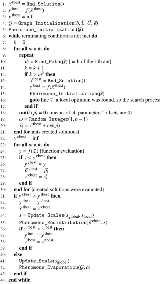
The version of DASA used in our experimental evaluation is described in details by Korošec et al. [8] (see Figure 1).

DASA introduces the concept of variable offsets (re-ferred as to parameter differences) for solving the continu-ous optimization problems. By utilizing discretized offsets of the real-valued problem parameters, the continuous op-timization problem is transformed to a graph-search prob-lem. More precisely, assuming a multidimensional param-eter space with xi being the current solution for the i-th

parameter, we define new solutionsx0_ias follow:

x0_i=xi+ωδi, (1)

whereδiis called the parameter difference and is selected

from the following set:

∆i= ∆−i ∪ {0} ∪∆

+

i , (2)

where

∆−_i ={δ_i,k− |δ_i,k− =−bk+Li−1_{, k= 1,2, . . . , d}

i} (3)

and

∆+_i ={δ+

i,k|δ

+

i,k=b

k+Li−1_{, k= 1,2, . . . , d}

i}. (4)

Here,

di=Ui−Li+ 1, (5)

Li=blogb(i)c, (6)

Ui=blogb(max(xi)−min(xi))c, (7)

i = 1,2, . . . , D,D is dimension of the problem,b is the discretization base,is the maximal computer arithmetic’s precision, and the weightω=Random_Integer(1, b− 1) is added to enable a more flexible movement over the search space.

In principle, DASA relies on two distinctive characteris-tics, differential graph and continuous pheromone model. Here, we will briefly discuss these two characteristics and outline the main loop of the DASA search process.

1:

~

x

tbest

=

Rnd_Solution

()

2:

y

best

=

f (

~

x

tbest

)

3:

y

tbest

=

inf

4:

_G

=

Graph_Initialization

(b,

~

L,

U,

~

~ǫ)

5:

Pheromone_Initialization

(

_G

)

6:

while terminating condition is not met do

7:

k

=

0

8:

for all m ants do

9:

repeat

10:

~

p

i

=

Find_Path

(

G

)

{

path of the i-th ant

}

11:

k

=

k

+

1

12:

if k

>

m

2

then

13:

~

x

tbest

=

Rnd_Solution

()

14:

y

best

=

f (

~

x

tbest

)

15:

Pheromone_Initialization

(

_G

)

16:

goto line 7

{

a local optimum was found, so the search process is restarted

}

17:

end if

18:

until (

p

~

i

=

0)

{

means of all parameters’ o

ff

sets are 0

}

19:

ω

=

Random_Integer

(1

,

b

₋

1)

20:

~

x

i

=

~

x

tbest

+

ωδ(~

p)

21:

end for

_{

ants created solutions

_}

22:

y

cbest

=

inf

23:

for all m ants do

24:

y

=

f (

~

x

i

)

{

function evaluation

}

25:

if y

<

y

cbest

then

26:

y

cbest

=

y

27:

~

p

cbest

=

~

p

i 28:

~

x

cbest

=

~

x

i 29:

end if

30:

end for

{

created solutions were evaluated

}

31:

if y

cbest

<

y

tbest

then

32:

y

tbest

=

y

cbest

33:

~

x

tbest

=

~

x

cbest

34:

s

=

Update_Scales

(s

_global

,

s

_local

)

35:

Pheromone_Redistribution

(~

p

cbest

,

s)

36:

if y

tbest

<

y

best

then

37:

y

best

=

y

tbest 38:

~

x

best

=

~

x

tbest 39:

end if

40:

else

41:

Update_Scale

(s

_global

)

42:

Pheromone_Evaporation

(

_G

,

ρ)

43:

end if

44:

end while

6

Second, DASA performs pheromone-mediated search that involves best-solution-dependent pheromone distribu-tion. The amount of pheromone is distributed over the ver-tices according to the Cauchy Probability Density Function (CPDF) [9]. DASA maintains a separate CPDF for each parameter. Initially, all CPDFs are identically defined by a location offset set to zero and a scaling factor set to one. As the search process progresses, the shape of the CPDFs changes: CPDFs shrink and stretch as the scaling factor de-creases and inde-creases, respectively, while the location off-sets move towards the offoff-sets associated with the better so-lutions. The search strategy is guided by three user-defined real positive factors: the global scale increase factor,s+,

the global scale decrease factor, s−, and the pheromone evaporation factor, ρ. In general, these three factors de-fine the balance between exploration and exploitation in the search space. They are used to calculate the values of the scaling factor and consequently influence the dispersion of the pheromone and the moves of the ants.

Finally, the main loop of DASA consists of an iterative improvement of a temporary-best solution, performed by searching appropriates paths in the differential graph. The search is carried out bymants, all of which move simul-taneously from a starting vertex to the ending vertex at the last level, resulting in m constructed paths. Based on the found paths, DASA generates and evaluates mnew can-didate solutions. The best among the m evaluated solu-tions is preserved and compared to the temporary-best so-lution. If it is better than the temporary-best solution, the latter is replaced, while the pheromone amount is redis-tributed along the path corresponding to the path of the pre-served solution and the scale factor is accordingly modified to improve the convergence. If there is no improvement over the temporary-best solution, then the pheromone dis-tributions stay centered along the path corresponding to the temporary-best solution, while their shape shrinks in or-der to enhance the exploitation of the search space. If for some fixed number of tries all the ants only find paths com-posed of zero-valued offsets, the search process is restarted by randomly selecting a new temporary-best solution and re-initializing the pheromone distributions.

3

Parameter Tuning

To obtain the best possible performance on a given prob-lem, one should consider a task specific tuning of the pa-rameter setting for the optimization algorithm used. Deter-mining the optimal parameters is an optimization task in it-self, which is extremely computationally expensive. There are two common approaches for choosing parameters val-ues: parameter tuning and parameter control. The first ap-proach selects the parameter settings before running the op-timization algorithm (and they remain fixed while perform-ing the optimization). The second approach optimizes the algorithm’s parameters along with the problem’s parame-ters. Here, we will focus on the first approach, parameter

tuning.

A detailed discussion and survey of parameter tuning methods is given by Eiben and Smit [4]. According to this survey, one way to approach parameter tuning is by sampling methods. Sampling methods reduce the search effort by decreasing the number of investigated parameter settings as compared to the full factorial design: the ba-sic full factorial design investigates2kparameter settings, subject tokparameters, each of which have2possible val-ues; in the more general case, parameters can have arbitrary number of values; moreover, an increase in the number of investigated parameters means an exponential increase in the number of parameter settings to be tested. Two widely used sampling methods are Latin-squares [9] and Taguchi orthogonal arrays [12]. However, these are not the most ro-bust sampling techniques, e.g., Latin-squares or Latin hy-percube sampling is good in the case where one of the pa-rameters dominates the algorithm’s performance, while it should be used with care if there are interactions among the parameters.

Ultimately, we would like to find a sampling schema that will be able to detect the interactions among the parame-ters, will be independent from user-specified information regarding the particular parameter values to be considered (typical for factorial design), and will deliver small but rep-resentative sample of the parameter search space. The first two requirements are satisfied by the pure random sam-pling, but the last is not, as random sampling does not guar-antee that the sampled values are evenly spread across the entire domain. The so-called low-discrepancy sequences were specially designed to fulfill all three requirements. Therefore, Sobol’ sequences, a representative variation of low-discrepancy sequences introduced by Sobol’ [10], was considered for sampling the parameter space of DASA in this study.

Sobol’ sequences, sampled from a D-dimensional unit search space, are quasi-random sequences ofD-tuples that are more uniformly distributed than uncorrelated random sequences of D-tuples. These sequences are neither ran-dom nor pseudo-ranran-dom: they are cleverly generated not to be serially uncorrelated by taking into account which tu-ples in the search space have already been sampled. For a detailed explanation and overview of the schemas for gen-erating Sobol’ sequences, we refer to [9]. The particular implementation of Sobol’ sampling used in our analysis is based on the Gray code order [5].

4

Experimental Evaluation

Table 1: Parameter settings for DASA* and DASA◦

Algorithm DASA◦ DASA*

Parameter D= 20 D= 40 D= 20 D= 40

m 10 10 5 7

ρ 0.2 0.2 0.324 0.388

s+ 0.02 0.02 0.201 0.136

s− 0.01 0.01 0.289 0.344

b 10 10 6 8

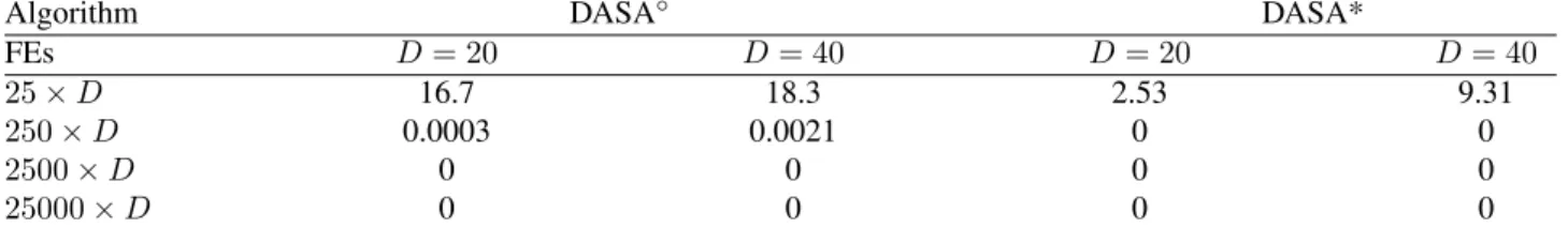
Table 2: Median values of the function errors for the Sphere function

Algorithm DASA◦ DASA*

FEs D= 20 D= 40 D= 20 D= 40

25×D 16.7 18.3 2.53 9.31

250×D 0.0003 0.0021 0 0

2500×D 0 0 0 0

25000×D 0 0 0 0

Therefore, the performance of DASA was evaluated on the Sphere function:

f(x) =|z|2+f(xopt), (8)

wherez = x−xopt andxopt is optimal solution vector,

such thatf(xopt)is minimal. Functionf(x)is defined over

D-dimensional real-valued search space x and is scalable with the dimension D. It has no specific value of its optimal solution (it is randomly shifted inx-space) and has an artifi-cially chosen optimal function value (it is randomly shifted inf-space). In this study, we considered the Sphere func-tion with respect to two dimensions,D= 20andD= 40. The performance of DASA is dependent on the values of five parameters: three real-valued parameters that directly influence the search heuristic (s+, s−, and ρ) and two

integer-valued parameters (mandb). Therefore, we con-sidered all of them for tuning DASA performance on the Sphere function for both search space dimensions,D= 20

andD = 40. Using the Gray-code-based Sobol’ genera-tor we generated 5000 parameter settings (5-tuples). Note that the Sobol’ sampling generates numbers on the unit in-terval: in order to obtain the true parameter settings, we mapped these values on the predefined search range of pa-rameter values. The latter for each of the five tuned param-eters was defined as follows: 4 ≤ m≤ 200,0 ≤ρ ≤1,

0 ≤s+ ≤1,0 ≤s− ≤ρ, and2 ≤ b≤100. Moreover, the mapped values for the integer-valued parametersmand

b were rounded to the closest integer value. Finally, due to implementation reasons, the upper bound of the global scale decrease factors−was actually limited by the value of the evaporation factorρ.

In the next step, the performance of the Sobol’ sampled parameter settings were tested on the Sphere benchmark function. Due to the stochastic nature of DASA, every parameter setting was used in a multiple-run experimental evaluation. Each run included25000×Dfunction evalua-tions (FEs). The number of runs was set to15. The results

gathered by the parameter tuning process are most often subjected to ordinal data analysis, which includes ranking of the different sampled parameter sets according to some calculated statistics, e.g., best or mean performance of the algorithm in some predefined number of runs [13]. In this case, performance of the algorithm is expressed in terms of the function error, i.e., the difference between the ob-tained and optimal function value. In order to find a setting that will be satisfactory in terms of convergence speed, we captured the error values at four different time points, cor-responding to25×D,250×D,2500×D, and25000×D

FEs.

The optimal performing parameter setting was chosen based on the median best performance over all runs aggre-gated over all time points for a given dimension (D = 20

and D = 40). A common approach is to use the mean performance, but we took the median in order to avoid the problems that the mean has when observing large vari-ance in the function values across the runs. More precisely, given a function, an individual rank is assigned to every setting (out of5000) for the four time points. A single fi-nal rank is calculated by ranking the sum of the four in-dividual rankings assigned to the parameter settings. The best-ranked parameter setting for a given dimension defines instance of DASA referred to as DASA*.

The results of DASA tuning subject to ordinal data anal-ysis are presented in Tables 1 and 2. Table 1 reports the tuned parameter settings for both DASA* instances.

In addition, the default parameter setting for DASA from [8] is given as a reference for comparison. The correspond-ing instance is referred to as DASA◦.

< 1.0E-08 1.0E-06 ... 1.0E-04 … 11.0E-02 … 11.0E-01 … 1

1000 0 0 0 0 0

10000 0 1.5 2.5 3.5 24

100000 38 9 10.5 21 9

1000000 86 3 5.5 4 1.5

0% 20% 40% 60% 80% 100%

1.0E+03 1.0E+04 1.0E+05 1.0E+06

FEs

Error

> 1.0E+02

1.0E+01 … 1.0E+02

1.0E+00 … 1.0E-01

1.0E-01 … 1.0E-02

1.0E-02 … 1.0E-04

1.0E-04 … 1.0E-02

1.0E-06 ... 1.0E-08

< 1.0E-08

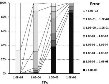
Figure 2: Median error distributions for the Sphere func-tion in the case ofD= 40.

5

Data Mining Analysis

Parameter tuning of an algorithm leads to a better per-formance, however it is a computationally expensive and problem-dependent task. Considering this, the idea is to extend the simple tuning that delivers a single parameter set and analyze the gathered data in an intelligent way. The intelligent analysis can extract patterns (regularities) in the explored parameter space that define a specific behavior of DASA. To this end, data mining methods for automated discovery of patterns in data can be used. As data mining methods can only discover patterns that are present in the data, the dataset subject to analysis must be large enough and informative enough to contain these patterns, i.e., to describe different types of algorithm’s behavior. Related to this, we considered a data mining approach on a represen-tative example, i.e., error model of the Sphere function.

To begin with, consider the graph in Figure 2 that visu-alizes the Sphere function error distribution. The graph de-picts the distribution of the median error values obtained by

5000parameter settings at four different points forD= 40. As we are more concerned with the practical significance between a large and a small error value than the statisti-cal significant difference between two actual error values, the error values are discretized into nine intervals, each of which is represented with a color chosen according to the error magnitude between black (error below10−8_{) and}

white (error above102_{). The graph clearly shows that the}

sampled settings determine different DASA performance. As evident, there is a big cluster of parameter settings that solve this function to the aimed accuracy (error below

10−8_{) in the given time budget (10}6_{FEs). Moreover, subset}

of this cluster solves the function for an order of magnitude less FEs. Our aim, therefore, is to find a (common) descrip-tion of this cluster, in terms of DASA parameter reladescrip-tions,

that represents a good behavior of DASA (as well as what parameter relations lead to a bad DASA performance).

For this purpose, we formulated the problem as a predic-tive modeling task using decision trees to model the func-tion error values in terms of the values of DASA parame-ters. Since the function error variables are continuous, the task at hand is a regression task. Furthermore, as our goal is to model the behavior of DASA at all time points simul-taneously, the problem at hand is then a multi-target re-gression. To this end, we used Predictive Clustering Trees (PCTs) which are implemented in Clus system [1]. In this case, the median error at the four time points define the four target attributes considered for modeling (with the PCT) in dependence from the descriptive attributes, i.e., the func-tion dimension and the five DASA parameters. The re-sulting dataset is composed of10002rows described with the5001parameter settings (including the default setting) of DASA applied to the two different dimensions, and10

columns corresponding to the10attributes.

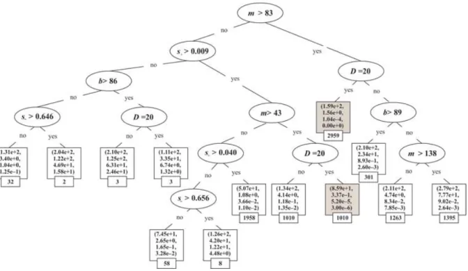
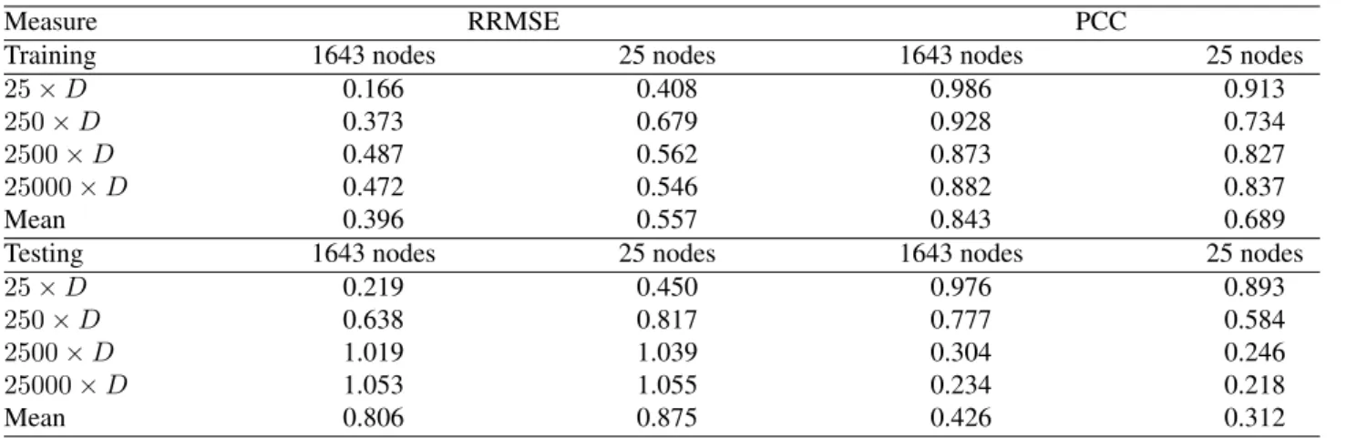
Figure 3 presents a PCT model for the Sphere function error. Each internal node of the tree contains a test on a descriptive attribute, while the leaves store the model pre-dictions for the function error, i.e., a tuple of four values. The predictions are calculated as the mean values of the corresponding error values for the data instances belonging to the particular leaf (represented by a box). In fact, each leaf identifies one cluster of data instances (the size of the cluster is the value in the small box). The predictive perfor-mance of the model was assessed with 10-cross-validation. Note that this particular model was learned on the com-plete dataset subject to constraints on the maximal tree size of25nodes. We did this because the original model con-tained 1643 nodes (of which822 leaves) and despite its better predictive performance, both training and testing, it was not comprehensible; aiming for an explanatory model, small and comprehensible, we considered the smaller tree obtained with the limitation of the size. The predictive per-formance of both models in terms of Root Relative Mean Squared Error (RRMSE) and Pearson Correlation Coeffi-cient (PCC) are given in Table 3. Note that RRMSE rep-resents the relative error with respect to the mean predictor performance, while PCC represents the linear correlation between the data and the model predictions. Good models have RRMSE values closer to0and PCC closer to1.

The model in Figure 3 outlines13 clusters of data in-stances, of which two (depicted with light-gray boxes) represent a good DASA performance. According to this model, the number of ants, m, is the most important DASA parameter for its performance on the Sphere func-tion. More precisely, ifm >83, independent of the values of the other parameters, DASA solves the 20-dimensional functional problem for the given time budget. Moreover, if m ≤ 83another DASA parameters become important as well. For example, if43 < m ≤ 83ands+ > 0.009

and D = 20then DASA solves the function with error

3 ×10−6, while the pattern m ≤ 43 ands≤0.040 and

regard-Figure 3: Predictive clustering tree representation of the error model for the Sphere function.

less of the function dimension. An interesting fact is that, the evaporation factor is not essential for DASA perfor-mance on the Sphere function. Moreover, the model also shows that is more difficult to describe the behavior of DASA for the 40-dimensional function problem than the 20-dimensional one.

Finally, note that the training performance (learned on the complete dataset) of the model in terms of the error and the correlation coefficient is best for the first target, while it gets worse with respect to the other three targets (see Ta-ble 3). This is especially significant if we take into account the testing performance of the model estimated with 10-cross-validation. However, the training performance is ac-ceptable in our case, as we are interested in understanding the behavior of DASA and not aiming to obtain a model for prediction.

6

Conclusion

The principle challenge of meta-heuristic design is provid-ing a default algorithm configuration, in terms of parameter setting, that will perform reasonably well in general (prob-lem) case. However, while it is a good initial choice, the default algorithm configuration may result in low quality solutions on a specific optimization problem. In practice, the algorithms parameters have to be fine-tuned in order to obtain best algorithm’s performance for the problem at hand, leading to the computational expensive task of pa-rameter tuning. So, if the tuning task is unavoidable, the question is: can we use the results from the parameter tun-ing to extract some knowledge about the algorithm’s

be-havior?

Related to this, the study focused on the problem of tun-ing the performance of the Differential Ant-Stigmergy Al-gorithm (DASA) with respect to its parameters. As it is the case with most of the meta-heuristic algorithms, the oper-ational behavior of DASA is determined by a set (five) of control parameters. The existing default setting of DASA parameters [8] is obtained by experimentation with both real and benchmark optimization problems, but not as a result of some systematic evaluation. Furthermore, there is no deeper understanding of the impact of a particular parameter or parameters relations on the performance of DASA. In this context, we performed a systematic evalua-tion of DASA performance obtained by solving the Sphere function optimization problem with 5000Sobol’ sampled DASA parameter settings regarding two dimensions, 20

and40.

Furthermore, we discussed the idea of learning a model of DASA behavior by data mining analysis of the parame-ter tuning results. In this context, we formulated the prob-lem as multi-target regression and applied predictive clus-tering trees for learning a model of DASA behavior with respect to the function error performance. The obtained model revealed that the parameter denoting number of ants is the most important parameter for DASA performance on the 20-dimensional function problem. On the other hand, the evaporation factor is not essential for DASA perfor-mance on the Sphere function.

fur-Table 3: Model performance with respect to RRMSE and PCC

Measure RRMSE PCC

Training 1643 nodes 25 nodes 1643 nodes 25 nodes

25×D 0.166 0.408 0.986 0.913

250×D 0.373 0.679 0.928 0.734

2500×D 0.487 0.562 0.873 0.827

25000×D 0.472 0.546 0.882 0.837

Mean 0.396 0.557 0.843 0.689

Testing 1643 nodes 25 nodes 1643 nodes 25 nodes

25×D 0.219 0.450 0.976 0.893

250×D 0.638 0.817 0.777 0.584

2500×D 1.019 1.039 0.304 0.246

25000×D 1.053 1.055 0.234 0.218

Mean 0.806 0.875 0.426 0.312

ther extended to building models of DASA behavior that will include the optimization problem characteristics (such as multimodality, separability, and ill-conditioning) as de-scriptive attributes as well. The latter can provide insights on how to configure DASA performance with respect to the type of the optimization problem. Moreover, these in-sights can serve as a valuable information for improvement of DASA design.

References

[1] H. Blockeel, J. Struyf (2002) Efficient Algorithms for Decision Tree Cross-validation,Journal of Machine Learning Research, vol. 3, pp. 621–650.

[2] C. Blum, A. Roli (2003) Metaheuristics in Combina-torial Optimization: Overview and Conceptual Com-parison,ACM Computing Surveys, vol. 35, no. 3, pp. 268–308.

[3] E. Bonabeau, M. Dorigo, G. Theraulaz (1999)Swarm Intelligence: From Natural to Artificial Systems, Ox-ford University Press.

[4] A. E. Eiben, S. K. Smit (2011) Parameter Tuning for Configuring and Analyzing Evolutionary Algorithms, Swarm and Evolutionary Computation, vol. 1, no. 1, pp. 19–31.

[5] S. Joe, F. Y. Kuo (2008) Constructing Sobol Se-quences with Better Two-dimensional Projections, SIAM Journal on Scientific Computing, vol. 30, no. 5, pp. 2635–2654.

[6] P. Korošec (2006) Stigmergy as an Approach to Metaheuristic Optimization, Ph.D. dissertation, Jožef Stefan International Postgraduate School, Ljubljana, Slovenia.

[7] P. Korošec, J. Šilc (2008) Using Stigmergy to Solve Numerical Optimization Problems, Computing and Informatics, vol. 27, no. 3, pp. 341–402.

[8] P. Korošec, J. Šilc, B. Filipiˇc (2012) The Differential Ant-stigmergy Algorithm,Information Sciences, vol. 192, no. 1, pp. 82–97.

[9] W. H. Press, S. A. Teukolsky, W. T. Vetterling, B. P. Flannery (1992)Numerical Recipes, Cambridge Uni-versity Press.

[10] I. M. Sobol’ (1967) Distribution of Points in a Cube and Approximate Evaluation of Integrals,USSR Com-pututational Mathematics and Mathematical Physics, vol. 7, no. 4, pp. 86–112.

[11] R. Stoean, T. Bartz-Beielstein, M. Preuss, C. Stoean (2009) A Support Vector Machine-Inspired Evolu-tionary Approach for Parameter Setting in Meta-heuristics, CIOP Technical report 01/09, Faculty of Computer Science and Engineering Science, Cologne University of Applied Science, Germany.

[12] G. Taguchi, T. Yokoyama (1993) Taguchi Methods: Design of Experiments, ASI Press.

[13] E.-G. Talbi (2009) Metaheuristics: From Design to Implementation, John Wiley & Sons.