Counterexamples in Model Checking - A survey

Counterexamples in Model Checking – A Survey

Hichem Debbi

Department of Computer Science, University of Mohamed Boudiaf, M’sila, Algeria E-mail: [email protected]

Overview paper

Keywords:model checking, counterexamples, debugging

Received:December 9, 2016

Model checking is a formal method used for the verification of finite-state systems. Given a system model and such specification, which is a set of formal properties, the model checker verifies whether or not the model meets the specification. One of the major advantages of model checking over other formal methods its ability to generate a counterexample when the model falsifies the specification. Although the main purpose of the counterexample is to help the designer to find the source of the error in complex systems design, the counterexample has been also used for many other purposes, either in the context of model checking itself or in other domains in which model checking is used. In this paper, we will survey algorithms for counterexample generation, from classical algorithms in graph theory to novel algorithms for producing small and indicative counterexamples. We will also show how counterexamples are useful for debugging, and how we can benefit from delivering counterexamples for other purposes.

Povzetek: Pregledni ˇclanek se ukvarja s protiprimeri v formalni metodi za preverjanje konˇcnih avtomatov, tj. sistemov manjše raˇcunske moˇci kot Turingovi stroji. Protiprimeri koristijo snovalcem na veˇc naˇcinom, predvsem kot naˇcin preverjanja pravilnosti delovanja.

1

Introduction

Model checking is a formal method used for the verification of finite-state systems. Given a system model and such spe-cification, which is a set of formal properties in temporal logics like LTL [109] and CTL [28, 52], the model checker verifies whether or not the model meets the specification. One of the major advantages of model checking over ot-her formal methods its ability to generate a counterexample when the model falsifies such specification. The counterex-ample is an error trace, by analysing it, the user can locate the source of the error. The original algorithm for counte-rexample generation was proposed by [31], and was imple-mented in most symbolic model checkers. This algorithm of generating linear counterexamples for ACTL, which is a fragment of CTL, was later extended to handle arbitrary ACTL properties using the notion of tree-like counterex-amples [36]. Since then, many works have addressed this issue in model checking. Counterexample generation has its origins in graph theory through the problem of fair cy-cle and Strongly Connected Component (SCC) detection, because model checking algorithms of temporal logics em-ploy cycle detection and technically a finite system model is determining a transition graph [32]. The original algo-rithm for fair cycle detection in LTL and CTL model was proposed by [53]. Since then, many variants of this algo-rithm and new alternatives were proposed for LTL and CTL model checking. In section 3 we will investigate briefly the problem of fair cycles and SCCs detection.

While the early works introduced by [28, 52] have inves-tigated the problem of generating counterexample so wi-dely, which led to practical implementation within well-known model checkers, the open problem that emerged was the quality of the counterexample generated and how it really serves the purpose. Therefore, in the last decade many papers have considered this issue, earlier in terms of structure[36], by proposing the notion of tree-like counte-rexamples to handle ACTL properties, and followed later by the works investigating the quality of the counterexam-ple mostly in terms of length to be useful later for debug-ging. In section 3, we will investigate the methods propo-sed for generating minimal, small and indicative counterex-amples in conventional model checking. Model checking algorithms are classified in two main categories, explicit and symbolic. While explicit algorithms are applied di-rectly on the transition system, symbolic algorithms em-ploy specific data structures. Generally, the explicit algo-rithms are adopted for LTL model checking, whereas sym-bolic algorithms are adopted for CTL model checking. In this section, the algorithms for generating small counte-rexamples are presented with respect to each type of al-gorithms.

to localize the source of the error given counterexamples. In this section, we consider that most of these methods range into two main categories: those that are applied on the counterexample itself without any need to other infor-mation, and those that require successful runs or witnesses to be compared with the counterexamples.

Probabilistic model checking has appeared as an exten-sion of model checking for analyzing systems that exhi-bit stochastic behavior. Several case studies in several domains have been addressed from randomized distribu-ted algorithms and network protocols to biological sys-tems and cloud computing environments. These syssys-tems are described usually using Discrete-Time Markov Chains (DTMC), Continuous Time Markov Chains (CTMC) or Markov Decision Processes (MDP), and verified against properties specified in Probabilistic Computation Tree Lo-gic (PCTL)[78] or Continuous Stochastic LoLo-gic (CSL) [9, 10]. In probabilistic model checking (PMC) ample generation has a quantitative aspect. The counterex-ample is a set of paths in which a path formula holds, and their accumulative probability mass violates the probabi-lity bound. Due to its specific nature, we specify section 5 for counterexample generation in probabilistic model checking. As it was done in conventional model checking, addressing the error explanation in the probabilistic mo-del checking is highly required, especially that probabilis-tic counterexample consists of multiple paths instead of a single path, and it is probabilistic. So, in this section we will also investigate the counterexample analysis in PMC.

The most important thing about counterexample is that it does not just serve as a debugging tool, but it is also used to refine the model checking process itself, through Coun-terexample Guided Abstraction Refinement(CEGAR)[37]. CEGAR is an automatic verification method mainly propo-sed to tackle the problem of state-explosion problem, and it is based on the information obtained from the counterex-amples generated. In section 6, we will show how counte-rexample contributes to this famous method of verification.

Testing is an automated method used to verify the qua-lity of software. When we use model checking to generate test cases, this is called model-based testing. This met-hod has known a great success in the industry through the use of famous model checkers such as SPIN, NuSMV and Java Pathfinder. Model checking is used for testing for two main reasons: first, because model checking is fully auto-mated, and secondly and more importantly because it de-livers counterexamples when the property is not satisfied. In section 7, we will show how counterexample serves as a good tool for generating test cases.

Although counterexample generation is in the heart of model checking, not all model checkers deliver counte-rexamples to the user. In the last section, we will review the famous tools that generate counterexamples. Section 9 concludes the paper, where some brief open problems and future directions are presented.

2

Preliminaries and definitions

Kripke Structure. A Kripke structure is a tuple M = (AP, S, s0, R, L)that consists of a setAP of atomic

pro-positions, a set S of states, s0 ∈ S an initial state, a

to-tal transition relationR ⊆S×S and a labelling function

L : W → 2AP that labels each state with a set of atomic propositions.

Büchi Automaton. A Büchi automaton is a tupleB = (S, s0, E,P, F)whereSis a finite set of states,s0∈Sis

the initial state,E ⊆S×Sis the transition relation,P_is

a finite alphabet, andF ⊆Sis the set of accepting or final states.

We use Büchi automaton to define a set of infinite words of an alphabet. A path is a sequence of states(s0s1...sk),

k ≥1such that(si, si+1)∈Efor all1 ≤i < k. A path

(s0s1...sk)is a cycle ifsk =s1, the cycle is accepting if it

contains a state inF. A path(s0s1...sk....sl)wherel > k

is accepting if sk...sl forms an accepting cycle. We call

a path that starts at the initial state and reaches an accep-ting cycle an accepaccep-ting path or counterexample (see Figure 1). A minimal counterexample is an accepting path with a minimal number of transitions.

Strongly Connected Component. A graph is a pairG= (V, E), whereV is a set of states andE ⊆ V ×V is the set of edges. A path is a sequence of states(v1, ..., vk),

k ≥ 1such that(vi, vi+1) ∈ E for all1 < i ≤ k. Let

π be a path, the length ofπis defined by the number of transitions and is denoted by[π]. We say that we can reach a vertexufrom a vertexvif there exists a path fromvto

u. We define a Strongly Connected Component (SCC) as a maximal set of statesC ⊆V such that for every pair of verticesu, v∈C,uandvare mutually reachable. A SCC C is trivial ifC ={v}, or otherwiseCis non-trivial if for everyu, v∈Cthere is a non-trivial path fromutov.

Discrete-Time Markov Chain (DTMC)A Discrete-Time Markov Chain (DTMC) is a tuple D = (S, sinit, P, L),

such that S is a finite set of states, sinit ∈ S the initial

state,P : S×S → [0,1]represents the transition proba-bility matrix, L : S → 2AP _{is a labelling function that}

assigns to each states ∈ Sthe setL(s)of atomic propo-sitions. An infinite pathσis a sequence of statess0s1s2...

, whereP(si, si+1)>0for alli ≥0. A finite path is the

finite prefix of an infinite path. We define a set of paths starting from a states0byP aths(s0). The probability of a

finite path is calculated as follows:

P(σ∈P aths(s0)|s0s1...snis a prefix ofσ) = Q

i≤0<nP(si, si+1)

Linear Temporal Logic (LTL) The syntax of LTL state formula over the setAPis given as follows :

ϕ::=true|a|¬ϕ|ϕ1∧ϕ2| ϕ|ϕ1U ϕ2

Figure 1: Accepting path (Counterexample).

alwaysoperatorGcan be easily derived using the temporal operatorU.

Given a pathπ = s0s1... and an integerj ≥ 0, where

π[j] =sj, such thatW ords(ϕ) ={π∈(2AP)w)σ|=ϕ},

the semantics of LTL formulas for infinite words over2AP

is given as follows:

π|=true⇔true π|=a⇔a∈L(s0)

π|=¬ϕ⇔π6|=ϕ

π|=ϕ1∧ϕ2⇔s|=ϕ1∧s|=ϕ2

π|=ϕ⇔π[1..]|=ϕ

π|=ϕ1Uϕ2⇔ ∃j≥0.π[j..]|=ϕ2∧(∀0≤k <

j.π[k..]|=ϕ1)

The semantics for the derived operatorsFandGis given as follows :

π|=F ϕ⇔ ∃j≥0.π[j..]|=ϕ π|=Gϕ⇔ ∀j≥0.π[j..]|=ϕ

Verifying whether a finite state system described in Kripke structureAM satisfies an LTL propertyϕreduces

to the verification thatA = AM ∩A¬ϕhas no accepting

path, whereA¬ϕrefers to the Büchi automaton that

viola-tesϕ,Lω(A) =W ords(¬ϕ). We call this procedure a test

of emptiness. So, in caseAM∩A¬ϕ6=∅, a counterexample

is generated.

Computation Tree Logic (CTL). We use the Computation Tree Logic (CTL) to specify properties of systems descri-bed using Kripke Structures. The CTL formulas are evalu-ated over infinite computations produced by Kripke struc-tureK. A computation of a Kripke structure is an infinite sequence of statess0s1, ... such thatsi, si+1 ∈ R for all

i∈_N. We denote byP aths(s)the set of all paths starting ats. The syntax of CTL state formula over the setAP is given as follows:

φ::=true|a|¬φ|φ1∧φ2|∃ϕ|∀ϕ

wherea∈AP is an atomic proposition andϕis a path formula. The path formulas are formed according to the following grammar:

ϕ::=φ|φ1U φ2

We denote byK, s|=φthe satisfaction of CTL formula at a statesofK. The semantics defined by the satisfaction relation for a state formula is given as follows

K, s|=true⇔true K, s|=a⇔a∈L(s)

K, s|=¬φ⇔s6|=φ

K, s|=φ1∧φ2⇔s|=φ1∧s|=φ2

K, s|=∃ϕ⇔for someπ∈P aths(s),π|=ϕ K, s|=∀ϕ⇔for allπ∈P aths(s),π|=ϕ

Given a path π = s0s1... and an integer i ≥ 0, where

π[i] = si, the semantics of path formulas is given as

fol-lows:

K, π|=φ⇔π[1]|=φ

K, π|=φ1Uφ2⇔ ∃j≥0.π[j]|=φ2∧(∀0≤k <

j.π[k]|=φ1)

In case the Kripke structure violates the specification

K6|=φ, a counterexample will be generated.

Both LTL and CTL are considered as sub-logics or frag-ments of the logic CTL∗ [28, 52]. CTL is the subset of CTL∗where each path operatorandU must be imme-diately preceded by path quantifiers∀ or∃, whereas LTL is the subset of CTL∗ that consists of formulas that have the form∀f, wheref is a path formula in which the only state formulas are just atomic propositions [32].ACT Lis the analogue fragment of CTL and thus of CTL∗, where the only quantifier allowed is∀. Using CTL∗we can ex-press formulas of the form∀(F Gp)∨ ∀G(∃F p), which is a disjunction of LTL and CTL formula.

Probabilistic Computation Tree Logic (PCTL). Probabi-listic Computation Tree Logic (PCTL) [78] has appeared as an extension of CTL for the specification of systems that exhibit stochastic behavior. We use the PCTL to define quantitative properties of DTMCs. PCTL state formulas are formed according to the following grammar:

φ::=true|a|¬φ|φ1∧φ2|P∼p(ϕ)

Wherea∈APis an atomic proposition,ϕis a path for-mula,Pis a probability threshold operator,∼∈ {<,≤, > ,≥}is a comparison operator, andpis a probability thres-hold. The path formulas ϕare formed according to the following grammar:

ϕ::=φ1Uφ2|φ1Wφ2|φ1U≤nφ2|φ1W≤nφ2

Where φ1 and φ2 are state formulas andn ∈ N. As

in CTL, the temporal operators (Ufor strong until,Wfor weak (unless) until and their bounded variants) are requi-red to be immediately preceded by the operator P. The PCTL formula is a state formula, where path formulas only occur inside the operatorP. The operatorPcan be seen as a quantification operator for both the operators∀(universal quantification) and∃(existential quantification), since the properties are representing quantitative requirements.

The semantics of a PCTL formula over a states (or a path σ) in a DTMC modelD = (S, sinit, P, L)can be

defined by a satisfaction relation denoted by |=. The sa-tisfaction ofP∼p(ϕ)on DTMC depends on the probability

mass of a set of paths satisfyingϕ. This set is considered as a countable union of cylinder sets, so that, its measurability is ensured.

s|=true⇔true s|=a⇔a∈L(s)

s|=¬φ⇔s6|=φ

s|=φ1∧φ2⇔s|=φ1∧s|=φ2

s|=P∼p(ϕ)⇔P(s|=ϕ)∼p

Given a pathσ=s0s1...inDand an integerj≥0, where

σ[j] =sj, the semantics of PCTL path formulas for DTMC

is defined as for CTL as follows:

σ|=φ1Uφ2⇔ ∃j ≥0.σ[j]|=φ2∧(∀0≤k < j.σ[k]|=

φ1)

σ|=φ1Wφ2⇔σ|=φ1Uφ2∨(∀k≥0.σ[k]|=φ1)

σ|=φ1U≤nφ2⇔ ∃0≤j≤n.σ[j]|=φ2∧(∀0≤k <

j.σ[k]|=φ1)

σ|=φ1W≤nφ2⇔σ|=φ1U≤nφ2∨(∀0≤k≤

n.σ[k]|=φ1)

For specifying properties of CTMC, we use the Conti-nuous Stochastic Logic (CSL). CSL has the same syntax and semantics as PCTL, except that in CSL the time bound in bounded until formula can be presented as an interval of non-negative reals. Before verifying CSL properties over CTMC, the CTMC has to be transformed to its embed-ded DTMC. Therefore, further description of CTMC mo-del checking is beyond the scope of this paper. We refer to [9, 10] for further details.

Generally, two types of properties can be expressed using temporal logics: Safety andLiveness. Safety pro-prieties state that something bad never happens, a simple example of that is the LTL formula G¬errorthat means that error never occurs. Liveness properties state that so-mething good eventually happens, a simple example of that is the CTL formula(∀Greq→ ∀F grant)that means that every request is eventually granted.

3

Counterexamples generation

Counterexample generation has its origins in graph theory through the problem of cycle detection. Cycle detection is an important issue in the heart of model checking, either explicit or symbolic model checking. To deal with this is-sue, various algorithms were proposed for both LTL and CTL model checking. Explicit state model checking is ba-sed on Büchi automaton, which is a type of ω-automata. The fairness condition relies on several sets of accepting states, where the acceptance condition is visiting the accep-tance set infinitely often. So, a run is accepting if only if it contains a state in every accepting set infinitely often. As a result, the emptiness of the language is based on checking the non-existence of the fair cycle or equivalently the fair non-trivial strongly connected component (SCC) that inter-sects each accepting set. In the case of non-emptiness, the accepting run is a sign of property failure, and as a result it is rendered as an error trace. We call this error trace a counterexample. So, the counterexample is typically pre-sented by a finite stem followed by a finite cycle. Several

algorithms were proposed to find counterexamples in re-asonable time, where finding the shortest counterexample has been proved to be a NP-Complete problem [31, 82].

To find fair SCCs, Depth First Search (DFS) and Breadth First Search (BFS) algorithms are used. The main algo-rithm employing DFS is the Tarjan’s algoalgo-rithm [126] that is based on manipulating the states of the graph explicitly. This algorithm is used to generate linear counterexamples in LTL verification and showed promising results [43, 129]. It is also adopted in probabilistic model checking to gene-rate probabilistic counterexamples for lower-bounded pro-perties, through finding bottom strongly connected com-ponents (BSCCs)[5]. BSCC is defined as an SCC B from which no state outside B is reachable from B. Finding the set of BSCCs over the probabilistic models is an important issue for the verification of PCTL and CSL properties. Tar-jan’s algorithm runs in linear time, but as the number of states grows, it simply becomes infeasible. As a result, the symbolic-based algorithms are proposed as a solution.

In contrast to explicit algorithms, symbolic algorithms [17, 19] employ BFS and can describe large sets in a com-pact manner using characteristic functions. Several symbo-lic algorithms were proposed for computing the set of states that contains all the fair SCCs, without enumerating them [32, 84, 128]. We refer to these algorithms as SCC-hull al-gorithms. Currently, most of the symbolic model checkers are employing Emerson’s algorithm due to its high perfor-mance, and it was proven by [58] that both of the algo-rithms [52] and [31] can work in a complementary way. Other works [83, 136] proposed algorithms based on enu-merating the SCCs, we refer to these algorithms as symbo-lic SCC-enumeration algorithms.

Different approaches for generating counterexamples are proposed regarding the two types presented before. Clarke et al. [31] proposed a hull-based approach based on Emer-son’s algorithm by searching a cycle in a fair SCC close to the initial state. Another approach by Hojati [84] was also employed by other works for generating counterexam-ples that use isolations techniques of the SCCs [95]. Using Emerson’s algorithm in a combinatory way with SCC-Enumeration algorithm is possible, but is still not guaran-teed to get a counterexample of short length. Ravi et al. [111] introduced a careful analysis of each type of these al-gorithms. Since there is no guarantee to find terminal SCCs close to the initial state, finding short counterexamples was still a trade-off and an open problem, and thus it was in-vestigated later by many researchers in both explicit and symbolic model checking.

3.1

Short counterexamples in explicit-state

model checking

A counterexample in the Büchi automaton is a pathσ=βγ

for-1: procedureDFS(s) 2: Mark(hs,0i)

3: for eachsuccessortofsdo

4: ifht,0inot marked then

5: DFS(t)

6: end if

7: end for

8: ifaccepting(s) thenseed:=s;NDFS(s) 9: end if

10: end procedure 11: procedureNDFS(s) 12: Mark(hs,1i)

13: for eachsuccessortofsdo

14: ifht,1inot marked then

15: NDFS(t)

16: else

17: if(t==seed)thenreport cycle

18: end if

19: end if

20: end for

21: end procedure

Figure 2: Nested Depth First Search Algorithm[130].

mally, a counterexampleσ=βγis minimal if(|β|+|γ|)≤

(|β0|+|γ0|)for any pathσ0=β0γ0. With respect to this de-finition, a counterexample has at least one transition. Many algorithms consider the issue of generating counterexam-ples given Büchi automaton [130, 85, 112]. All these works employ Nested-Depth First Search (NDFS), but they are not capable of finding a minimal counterexample. A basic NDFS algorithm proposed by [130] is depicted in Figure 2. The algorithm is based on computing the accepting sta-tes by performing a simple search, once an accepting state is found, another search is performed to find an accepting cycle through it.

Although minimal counterexamples can be computed in polynomial time using minimal paths algorithms, the main drawback, in fact, is the memory, where the resulting Bü-chi automaton to be checked for emptiness is usually very huge, the thing that makes storing all the minimal paths to be compared so difficult.

Recently, new methods were proposed to compute mi-nimal counterexample in Büchi automaton [77, 64, 63]. Hansen and Kervinen [77] proposed a DFS algorithm that runs in O(n2_{)and they showed that O(nlogn) is}

suffi-cient, although DFS algorithms are memory consuming in general. This is due to the optimizations added using in-terleaving. Since the algorithms are based on exploring transitions backwards, adapting this method in practice is very difficult, especially by considering some restrictions. While this method requires more memory than the model checker SPIN does, [64, 63] proposed a method that does not use more memory than SPIN does. While the first one uses DFS and its time complexity is exponential [64], Gas-tin and Moro proposed a BFS algorithm with some optimi-zations able of computing the minimal counterexample in

polynomial time [63]. Hansen et al. [76] also proposed a method for computing minimal counterexamples based on Dijkstra algorithm for detecting strongly connected com-ponents. A novel approach was proposed by [93] for gene-rating short counterexamples based on analyzing the entire model and defining which events have more contribution to the error, these events are called crucial. In addition to generating short counterexamples, the technique helps with reducing the state space. The main drawback of this met-hod is how to determine if such set of events are crucial and really led to the error.

3.2

Short counterexamples in symbolic

model checking

The original algorithm for counterexample generation in symbolic model checking was proposed by [31] and was implemented in most symbolic model checkers. This al-gorithm of generating linear counterexamples for the linear fragment of ACTL was later extended to handle arbitrary ACTL properties using the notion of tree-like counterex-amples [36]. The authors realized that linear counterexam-ples are very weak for ACTL, and thus they proposed to generate tree-like Kripke structure instead, which is proven to be a viable counterexample[36, 38]. Formally, a tree-like counterexample is a a directed tree whose SCCs are either cycles or simple nodes. Figure 3 shows an exam-ple of a tree-like counterexamexam-ple for the ACTL property ∀G¬a∨ ∀F¬b. As we see in the figure, the counterexam-ple consists of two paths refuting both subformulas. The first path leads to a state that satisfiesa, whereas the se-cond path, which is expected to be an infinite one, along whichbalways holds. The generic algorithm for generating tree-like counterexamples as proposed in [36] is depicted in Figure 4.

Figure 3: A tree-like counterexample for∀G¬a∨ ∀F¬b.

The counterexample is constructed from an indexed Kripke structureKω _{that is obtained by creating}

operator, andCis a global variable that is used in unrave-ling through denoting index of states.

The algorithm outputs a sequence of descriptorsof the form< s0, .., sn >(path descriptor) and< s0, .., sn, s0>

(loop descriptor), where S_{{desc1, desc2}}

describes a fi-nite path leading to a cycle. The tree-like counterexample will be thenS Q_{, where}Q_{refers to the set of descriptors}

generated by CEX algorithm. The set of descriptors for the example in Figure 3 would be:< s0, s1, s2>,< s0, s3>

and< s3, s4, s5>ω.

1: procedure CEX(K,si0,ϕ)

2: caseϕof

3: ϕ1∨ϕ2:

4: CEX(K,si

0,ϕ1)

5: CEX(K,si

0,ϕ2)

6: ∧i≥1ϕi: 7: ϕ1∧ϕ2:

8: Selectjsuch thatK, s06|=ϕj

9: CEX(K,si

0,ϕj) 10: ∀O(ψ1, ..., ψk):

11: Determine σ = s0, ..., sN, ..., sN+M such that

K, σ6|=O(ψ1, ..., ψk)

12: desc1:=hsi0, unravel(C, s1, ..., sN)i 13: desc2:=hunravel(C+N, sN, ..., sN+M)iω 14: returndesc1 and desc2

15: C:=C+N+M+ 1

16: for all statesp∈S{desc1, desc2}do 17: forj∈ {1, ..., k}do

18: ifK, p6|=ψjthen 19: CEX(K, p, ψj)

20: end if

21: end for

22: end for

23: end case

24: end procedure

Figure 4: The generic counterexample algorithm for ACTL[36].

After these works of Clarke et al., many works have ad-dressed the issue of computing short counterexamples in symbolic model checking [117, 29, 108]. Schuppan et al. [117] proposed some criteria that should be met for the Bü-chi automaton to accept shortest counterexamples. They proved that these criteria are satisfied in the approach pro-posed by [29] just for future time LTL specification, and thus they proposed an approach that meets the criteria posed for LTL specifications with past. The algorithm pro-posed employs breadth-first reachability check with Binary Decision Diagrams(BDD)-based symbolic model checker.

The authors in [108] proposed a black-box based techni-que that masks some parts of the system in order to give an understandable counterexample to the designer. So the work does not just tend to produce minimal counterexam-ples, but also, it delivers small indicative counterexample of good quality to be analyzed in order to get the source

of the error. The major drawback of this method is that the generalization of counterexample generation from sym-bolic model checking to black box model checking, could lead to non-uniform counterexamples that do not meet the behavior of the system intended. While all of these works are applied to unbounded model checking [117, 108], the works [122, 120, 113] consider bounded model checking, through lifting assignments produced by a SAT solver, where the quality of the counterexample generated depends on the SAT solver in use. Other works have investigated the use of heuristics algorithms for generating counterexam-ples [124, 50]. Although heuristics were not widely used, they gave pretty good results and were also used later for generating probabilistic counterexamples.

4

Counterexamples analysis and

debugging

One of the major advantages of model checking over ot-her formal methods is its ability to generate a counterex-ample when the model falsifies such specification. The counterexample represents an error trace; by analyzing it the user can locate the source of the error, and as Clarke wrote:“The counterexamples are invaluable in debugging complex systems. Some people use model checking just for this feature”[27].

However, generating small and indicative counterexam-ples only is not enough for understanding the error. There-fore, counterexamples explanation is inevitable. Error ex-planation is the task of discovering why the system exhibits this error trace. Many works have addressed the automatic analysis of counterexamples to better understand the fai-lure. Error explanation ranges in two main categories. The first is based on the error trace itself, through considering the small number of changes that have to be made in order to ensure that the given counterexample is no longer exhi-bited, and thus, these changes represent the sources of the error. The second is based on comparing successful execu-tions with the erroneous one in order to find the differen-ces, and thus those differences are considered as candidate causes for the error. Kumar et al. [97] have introduced a careful analysis of the complexity of each type. For the first type, they showed using three models (Mealy machi-nes, extended finite state machimachi-nes, and pushdown automa-ton) that this problem is NP-complete. For the second type, they provided a polynomial algorithm using Mealy machi-nes and pushdown automaton, but solving the problem was difficult with extended finite state machines.

second is that model checker usually floods the designer with multiple counterexamples, without any kind of clas-sification. This makes challenging the task of choosing a helpful counterexample for debugging purposes. Besides, a single counterexample it might not be enough to under-stand the behavior of the system. Analyzing a set of coun-terexamples together is an option but the problem is that it requires much effort, and even though, the set of counte-rexamples to be analyzed could contain the same diagnostic information, which may make analyzing this set of counte-rexamples a waste of time. The last and the most important problem in error explanation is that not all the events that occur on the error trace are of importance for the designer, so locating critical events is the goal behind error explana-tion. In this section, we survey some works with respect to the two categories.

4.1

Computing the minimal number of

changes

Jin et al. [92] proposed an algorithm for analyzing the counterexamples based on the local information, by seg-menting the events of the counterexamples in two main segments, fated and free. The fated segments refer to the events that obviously have to occur in the executions, and the free segments refer to the events that should be avoided for the error not to occur, and thus they are candidate to be causes. Fated and free segments are computed with respect to input variables in the system, where they are classified into controlling and non-controlling. While controlling va-riables are considered to be critical, and have more control on the environment, the non-controlling variables have less importance. So that, fated segments are determined with respect to controlling variables, whereas free segments are determined with respect to non-controlling ones.

Wang et al. [132] also proposed a method that works just on the failed execution path without considering successful ones. The idea is about looking at the predicates candidate for causing the failure in the error trace. To do so, they use weakest pre-condition computation, the technique that is widely used in predicate abstraction. This computation aims to find the minimal number of conditions that should be met in order to not let the program violate the asser-tion. This results in a set of predicates that contradict with each other. By comparing how these predicates contradict to each other, we can find the cause for the assertion fai-led and map it back to the real code. Many similar works also provided error explanation methods in the context of C programs [137, 127, 138].

Using the notion of causality by Halpern and Pearl [74], Beer et al. [88] introduced a polynomial-time algorithm for explaining LTL counterexamples that was implemented as a feature in the IBM formal verification platform Rule-Base PE. Given the error trace, the causes for the violation are highlighted visually as red dots on the error trace it-self. The question asked was: what values of signals on the trace cause it to falsify the specification? Following the

definition of Halpern and Pearl, they refer to such a set of pairs of state-variable as bottom-valued pairs whose values should be switched to make such state-variable pair criti-cal. The pair is said to be critical if changing the value of the variable in this state no longer produces a counterexam-ple. This pair represents the cause for the first failure of the LTL formula given the error trace, where they argue that the first failure is the most relevant to the user. Neverthe-less, the algorithm computes an over-approximation of the set of causes not just the first cause that occurred.

Let ϕ be an LTL formula in Negation Normal Form (NNF) andπ=s0, s1, ..., ska counterexample for it. The algorithm for computing the approximate set of causes gi-venϕandπis depicted in Figure 5. The procedure invokes each time a functionvalfor evaluating sub-formulas ofϕ

on the path. The procedure is executed recursively given the formulaϕuntil it reaches the proposition level, where the cause is finally rendered as a pairhsi, pi/hsi,¬pi, where

sirefers to the current state.

Let us consider the formula : G((¬ST ART ∧ ¬ST AT U S_V ALID ∧ EN D) →

[¬ST ARTUST AT U S_V ALID]). The result of executing the RuleBase PE implementation of the algo-rithm on this formula is shown in Figure 6. The red dots refer to the relevant causes for the error. Where some variables are not critical for the failure, others can be cri-tical, which means that switching their values alone could result in mitigating the violation. For instance, in state 9,

ST ART precedesST AT U S_V ALID, by switching the value ofST ART from 1 to 0 in state9, the formula would not fail anymore given this counterexample.

4.2

Comparing counterexamples with

successful runs

This is the most adopted method for error explanation that is successfully featured in many model checkers such as SLAM and Java PathFinder. Groce et al. [70] have propo-sed an approach for counterexamples explanation bapropo-sed on computing a set of faulty runs called negatives, in which the counterexample is included, and comparing it to a set of correct runs called positives. Analyzing the common features and differences could lead to getting a useful di-agnostic information. Their algorithms were implemented in JAVA pathfinder. Based on Lewis counterfactual the-ory of causality [105] and distance metrics, Groce [68] has proposed a semi-automated approach for isolating errors in ANSI C programs, by considering the alternative worlds as programs executions and the events as propositions about those executions. The approach relies on finding causal de-pendencies between predicates of a program. A predicate

ais causally dependent onbgiven the faulty execution, if only if the executions in which the removal of a causea

1: procedure CAUSES(ϕ,πi) 2: Caseϕof

3: p:

4: ifp6∈si then 5: returnhsi, pi 6: end if

7: ¬p:

8: ifp∈si then 9: returnhsi, pi 10: end if

11: Xϕ:

12: ifi < k then return Causes(ϕ,πi+1) 13: end if

14: ϕ∧ψ:

15: return Causes(ϕ,πi_{)∪Causes(ψ,π}i₎ 16: ϕ∨ψ:

17: ifval(ϕ, πi_{) = 0andval(ϕ, ψ}i_{) = 0 then} 18: return Causes(ϕ,πi_{)∪Causes(ψ,π}i₎ 19: end if

20: Gϕ:

21: ifval(ϕ, πi) = 0 then

22: return Causes(ϕ,πi₎ 23: else

24: if val(ϕ, πi) = 1 and i < k and

val(XGϕ, πi_{) = 1 then}

25: return Causes(Gϕ,πi+1₎

26: end if

27: end if

28: φUψ:

29: ifval(ϕ, πi) = 0andval(ψ, πi) = 0then

30: return Causes(ϕ,πi)∪Causes(ψ,πi) 31: ifval(ϕ, πi) = 1andval(ψ, πi) = 0andi=k

then

32: return Causes(ψ,πi₎ 33: end if

34: ifval(ϕ, πi) = 1andval(ψ, πi_{) = 0andi < k}

andval(X[ϕUψ], πi_{) = 0then}

35: return Causes(ψ, πi_{) ∪}

Cau-ses(πi+1_,[ϕUψ])

36: end if

37: end if

38: end procedure

Figure 5: Causes generation algorithm given a counterexample[88].

Figure 6: Explanations on counterexample as red dots[88].

approach is depicted in Figure 7.

Figure 7: Explanation using distance metric[68].

Given a programPand its specification, the model chec-ker CBMC is used to generate a counterexample through using SAT solver, where the counterexample represents a finite execution ofP. The explain tool[69] gets the coun-terexample generated from CBMC together with thePand its specification. It generates first a set of executions that do not violate the specification, and then using PBS solver [7], it tries to find the closest execution to the counterexample. Finally, the distance metric is computed, and a dynamic sli-cing technique is applied in order to point out to the most relevant assignments in the program that had contributed the most to the error.

Figure 8: An example of C program.

Figure 9: Counterexample values.

Figure 10: Successful execution values.

which is a representation used by CBMC (See Figure 9). A successful execution so close to the counterexample can be found for the input values (1,1,1) (See Figure 10). The change in the value ofinput2results in the assertion

least <= mostbeing true. The differences between the two executions are presented in Figure 11. The first change is in the value ofinput2, which results in the change of

most#1from 0 to 1. These two changes have of course lower importance to the following change, which concerns the non execution of guard#3that was executed in the counterexample, sinceleast#0 is no longer greater than

input2#0, and thus the value of#most6has changed to 1, which is considered the last change. The explanation that can be given for this counterexample, is that not exe-cuting the instruction at line 10 leads to the satisfaction of the assertion (no error occurring). This shows clearly the causal dependency of the satisfaction/violation of the as-sertion on executing this line of code. As a result, line 10 will be highlighted byExplaintool as an indication for the source of the error. The user will then understand that the this line of code should be corrected asleast=input2.

In [22], Chaki and Groce extended the original approach for comparing a counterexample with the closest success-ful run through combining distance metric with predicate abstraction in order to generate explanations for abstract counterexamples. They argue that even for abstract counte-rexample, abstract state-space makes the explanation more informative. Renieris and Reiss [114] also introduced a method based on distance metric to select the closest cor-rect runs to the faulty one and they provided a quantitative method for evaluating their methods.

Figure 11: Differences between the counterexample and the successful execution.

Ball et al. [11] proposed an effective approach that is currently featured in SLAM model checker. Their met-hod is based on the same principle of finding successful runs to be compared with the counterexample. The inte-resting difference here is that it generates error trace per error cause, which makes the diagnostic easier, since there will not be causal dependencies in the traces generated. It is clear that this method will require the invocation of the model checker each time a cause for the error is found. Finally, the causes are reported as erroneous transitions that do not occur in any correct trace. Copty et al. [41] proposed a framework for debugging counterexamples as they refer to it as counterexample Wizard in the context of symbolic LTL. The technique employs three main capabi-lities: multi-value counterexample annotation, constraint-based debugging and multiple counterexample generation. But in contrast to the work by Ball et all, the model chec-ker is not invoked each time an error cause is found, but instead, it gets all the data needed together to start the ana-lysis.

Leue and Tabaei Befrouei [104, 103] proposed a novel approach based on computing two datasets, the bad da-taset that represents the set of counterexamples, and the good datasetthat represents the successful runs. Both da-tasets are produced using SPIN model checker. The idea is always about computing the differences between good and bad traces, but this time with the help of data mining technique called sequential pattern mining [49]. The aim behind using this technique is to extract a set of sequences of actions that are mostly to appear in the bad dataset. In concurrent systems, which are usually modeled using in-terleaving semantics, the unforeseen inin-terleavings resulted from such a set of actions stand as a good indicator for the source of the error.

While all of the previous works addressed safety pro-perties, Kumazawa and Tamai [98] attended to explain er-rors for liveness properties that involve more computati-onal complexity. For that reason, the counterexample is represented as an infinite trace and not a finite one, and the witnesses to be compared with this counterexample are infinite as well. The method also employs shortest paths algorithms. Many similar works for counterexamples ana-lysis have been done [121, 73, 40, 110, 119, 118, 56, 45].

5

Probabilistic counterexamples

sin-gle path ending with a bad state representing the failure, the task in PMC is quite different. The counterexample in PMC is a set of evidences or diagnostic paths that sa-tisfy path formula and their probability mass violates the probability threshold. The probabilistic counterexample is generated when a PCTL/CSL property is not satisfied. The probabilistic propertyφ=P≤p(ϕ)is refuted when the

pro-bability mass of the paths satisfyingϕexceeds the bound

p. Therefore, a probabilistic counterexample for the pro-pertyφis formed by a set of paths starting at a statesand satisfying the path formula ϕ. We denote these paths by

P aths(s0 |=φ). The counterexample can be formed of a

set of finite paths where each pathσ=s0s1...snis a prefix

of an infinite path fromP aths(s0|=φ)satisfying the

for-mulaϕ. We denote these paths byF initeP aths(s0|=φ).

We can get a set of probabilistic counterexamples, noted

P CX(s0 |= φ), which is a set of any combination from

F initeP aths(s0|=φ)that their probability mass exceeds

the boundp. Among all these probabilistic counterexam-ples, we are interested by the most indicative one. The most indicative counterexample is minimal counterexample (has the least number of paths fromF initeP aths(s0|=φ)) and

its probability mass is the highest among all other minimal counterexamples. We denote the most indicative probabi-listic counterexample byM IP CX(s0 |= φ). We should

note that the most indicative probabilistic counterexample may not be unique.

For the counterexample to have a high probability, it should consist of paths that carry high probabilities from

F initeP aths(s0 |= φ). The path σ having the

hig-hest probability over all these paths is called strongest path and is defined as follows: for every path σ0 _∈

F initeP aths(s0 |= φ) : P(σ) ≥ P(σ0). The strongest

path also may not be unique.

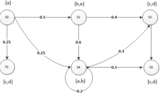
ExampleLet us consider the example of DTMC shown in Figure 12 and the property P≤0.5(ϕ), where ϕ =

(a∨b)∪(c∧d). The property above is violated in this model (s06|=P≤0.5(ϕ)), since there exists a set of paths satisfying

ϕ whose probability mass is higher than the probability bound (0.5). Any combination fromF initeP aths(s0 |=

φ)having probability mass higher than 0.5, is a valid coun-terexample including the whole set. For instance, we can find three counterexamples:

P(CX1) =

P({s0s1, s0s2s3, s0s2s4s3, s0s2s4s5, s0s4s5})

= 0.25 + 0.2 + 0.09 + 0.15 + 0.12 = 0.81

P(CX2) =P({s0s1, s0s2s4s5, s0s4s5})

= 0.25 + 0.15 + 0.12 = 0.52

P(CX3) =P({s0s1, s0s2s3, s0s2s4s5})

= 0.25 + 0.2 + 0.15 = 0.6

The last probabilistic counterexample is the most indi-cative since it is minimal and its probability is higher than

Figure 12: A DTMC.

the other minimal counterexampleCX2,P(CX3) = 0.6>

P(CX2). The strongest path iss0s1, which is included in

the most indicative probabilistic counterexample.

5.1

Probabilistic counterexample generation

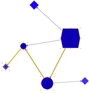
Various approaches for probabilistic counterexamples ge-neration have been proposed. Aljazzar et al. [1, 3] introdu-ced an approach for counterexample generation for DTMC and CTMC against timed reachability proprieties using heuristics and directed explicit state space search. Since resolving nondeterminism in an MDP results in a DTMC, in complementary work [4], Aljazzar and Leue proposed an approach for counterexample generation for MDPs ba-sed on existing methods for DTMC. Aljazzar and Leue in-troduced a complete work in [5] for generating counterex-amples for DTMCs and CTMSs as what they refer to as diagnostic sub-graphs. All these works on generating in-dicative counterexamples have led to the development of the K* algorithm [6], an on-the-fly heuristics guided al-gorithm for the K shortest path problem. Comparing to classical k-shortest-paths algorithms, K* has two main ad-vantages, it woks on-the- fly in way it avoids exploring the entire graph, and it can be guided using heuristic functions. Based on all the previous works, they built a tool DiPro [2] for generating indicative counterexamples for DTMCs, CTMCs and MDPs. This tool can be jointly used with the model checkers PRISM [81] and MRMC [94], and can ren-der the counterexamples in text format as well as in graphi-cal mode. These heuristic-based algorithms showed a great efficiency in terms of counterexample quality. Neverthe-less, with large models, DiPro tool that implements these algorithms takes usually a long time to produce a counte-rexample. By running DiPro on a PIRSM model of the DTMC presented in Figure 12 against the same property, we obtain the most indicative counterexampleCX3. The graphical representation ofCX3 as rendered by DiPro is depicted in Figure 13. The diamonds refer to the final or end states (s1,s3,s5), whereas the circles represent simple

nodess2 ands4. The user can navigate through the

coun-terexample and inspect all values.

redu-Figure 13: A counterexample generated by DiPro.

ces to the problem of finding K shortest paths. In a weigh-ted digraph transformed from the DTMC model, and given initial state and the target states, the strongest evidences that form the counterexample are selected using extensi-ons of K-shortest paths algorithms for an arbitrary number k. Instead of generating path-based counterexamples, [134] have proposed a novel approach for DTMCs and MDPs ba-sed on critical subsystems using SMT solvers and mixed integer linear programming. Critical subsystem is simply a part of the model (states and transitions) that are con-sidered relevant because of its contribution to exceeding the probability bound. The problem has been shown that is NP-Complete. Another work always based on the no-tion of critical subsystem is proposed to deliver abstract counterexamples with less number of states and transiti-ons using hierarchical refinement method. Based on all of these works, Jansen et al. proposed the COMICS tool for generating the critical subsystems that induce the counte-rexamples [90].

There are also many other works that addressed special cases for generating counterexamples in PMC. the authors of [8], proposed an approach for finding sets of evidences for bounded probabilistic LTL properties on MDP that be-have differently from each other giving significant diagnos-tic information. While their method is also based on K-shortest path, the main contribution is about selecting the evidences or the witnesses with respect to main five cri-teria in addition to the high probability. While all of the previous works for counterexample generation are explicit-based, the authors in [133] proposed a symbolic method using bounded model checking. In contrast to the previ-ous methods, this method lacks the selection of the stron-gest evidences first, since the selection is performed in ar-bitrary order. Another approach for counterexample gene-ration that uses bounded model checking has been

propo-sed [15]. Unlike the previous work that uses conventional SAT solvers, the authors used a SMT-solving approach in order to put some constraints on the paths selected, in order to get more abstract counterexample that consists of stron-gest paths. Counterexample generation for probabilistic LTL model checking has been addressed in [116] and pro-babilistic CEGAR has been also addressed [80]. A com-prehensive representation of the counterexamples using re-gular expressions has been addressed in [44]. Since regu-lar expressions deliver compact representations, they can help to deliver short counterexamples. Besides, they are widely known and easily understandable, so that they will give more benefits as a tool for error explanation.

5.2

Probabilistic counterexample analysis

Instead of relying on the state space search resulted from the parallel composition of the modules, [135] suggests to rely directly on the guarded command language used by the model checker, which is more likely and helpful for de-bugging purpose. To do so, the authors employ the critical subsystem technique [134] to identify the smallest set of guarded commands contributing to the error.

To analyze probabilistic counterexamples, Debbi and Bourahla [48, 47] proposed a diagnostic method based on the definition of causality by Halpern and Pearl [74] and responsibility [25]. The method proposed takes the pro-babilistic counterexample generated by DiPro tool and the probabilistic formula as input, and returns a set of pairs (state-variable) as candidate causes for the violation orde-red with respect to their contribution to the error. So, in contrast to the previous methods, this method does not tend to generate indicative counterexamples, but it acts directly on indicative counterexamples already generated. Another similar approach for debugging probabilistic counterexam-ples has been introduced by [46]. It adopts the same defi-nition of causality by Halpern and Pearl to reason formally about the causes, and then transforms the causality model into regression model using Structural Equation Modeling (SEM). SEM is a comprehensive analytical method used for testing and estimating causal relationships between va-riables embedded in theoretical causal model. This met-hod helps to understand the behavior of the model through quantifying the causal effect of the variables on the viola-tion, and the causal dependencies between them.

that could help the designer to get a better insight on the behavior of the system. They proved the applicability of their approach to many industrial size PROMELA models. They extended the causality checking approach to proba-bilistic counterexamples by computing the probabilities of events combination [101], but they still consider the use of causality checking of qualitative PROMELA models.

6

Counterexample guided

abstraction refinement (CEGAR)

The main challenge in model checking is the state explo-sion problem. Dealing with this issue is in the heart of model checking, it was addressed at the beginning of mo-del checking and not finished. Many methods were pro-posed to tackle this issue, the most famous are: symbolic algorithms, Partial Order Reduction (POR), Bounded Mo-del Checking (BMC) and abstraction. Among these techni-ques, abstraction is considered as the most general and flex-ible for handling the state explosion problem [30]. Ab-straction is about hiding or simplifying some details about the system to be verified, even removing some parts from it that are considered irrelevant for the property under con-sideration. The central idea is that verifying a simplified or an abstract model is more efficient than the entire model. Evidently, this abstraction has a price, which is losing some information, and the best abstraction methods are those that control this loss of information. Over-approximation and under-approximation are two main key concepts for this problem. Many abstraction methods have been proposed [42, 65, 106], the last one had the most attention and was adopted in the symbolic model checker NuSMV.

Abstraction can be defined by a set of abstract statesSb,

an abstraction mapping functionhthat maps the states in the concrete model to Sb, and the set of atomic

propositi-onsAP labeling these states. Regarding the choice onSb,

handAP, we distinguish three main types of abstraction : predicate abstraction [66, 115], localization reduction [99] and data abstraction [39]. Predicate abstraction is based on eliminating some variables from the program to be re-placed by predicates that still serve the information about these variables. Each predicate has a Boolean variable cor-responding to it, where the abstract states Sb resulted are

valuations of these variables. Both the abstraction map-pinghbetween the concrete and abstract states, and the set of atomic propositionsAP, are determined with respect to the truth values of these predicates. The entire abstract mo-del can then be defined through existential abstraction. To this end, we can use BDDs, SAT solvers or theorem pro-vers depending on the size of the program. Localization reduction and data abstraction are actually just extensions of predicate abstraction. Localization reduction aims to de-fine a small set of variables that are considered relevant to the property in hand to be verified, these variables are cal-led visible, the rest of variables that have no importance with respect to the property to be verified are called

invisi-ble. We should mention that this technique does not apply any abstraction on the domain of visible variables. Data ab-straction deals mainly with the domains of variables by ma-king an abstract domain for each variable. So the abstract model will be built with respect to the abstract values. For more detail on abstraction techniques, we refer to [71].

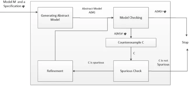
Given the possible loss of information caused by the abstraction, inventing some refinement methods of the abstract model is necessary. The most known method for abstraction refinement is Counterexample-Guided Ab-straction Refinement (CEGAR) that has been proposed by [30] as a generalization of the localization reduction ap-proach. A prototype implementation of this method in NuSMV has also been presented. In this approach, the counterexample plays the crucial role for finding the right abstract model. The process of CEGAR consists of three main steps: the first is to generate an abstract model using one of the abstractions techniques [30, 23, 33] given a for-mulaϕ. The second step is about checking the satisfaction ofϕ, if it is satisfied then the model checker stops and re-turns that the concrete or the original model satisfies the formula, if it is not satisfied, a counterexample will be ge-nerated. The counterexample generated is in the abstract model, so we have to check if it is also a valid counterex-ample in the concrete model, because the abstract model has different behavior comparing to the concrete one. Ot-herwise, the counterexample is called spurious and the ab-straction must be carried out based on this counterexample. So, a spurious counterexample is an erroneous counterex-ample that exists only in the abstract model, not the con-crete model. The final step is to refine the model until no spurious counterexample is found (see Figure 14). This is how the technique gets its name, refining the abstract mo-del using the spurious counterexample. Refinement is an important task of CEGAR that can make the process faster and gives the appropriate results. To refine the abstract mo-del, different partitioning algorithms are applied to abstract states. Like abstraction, partitioning the abstract states in order to eliminate the spurious counterexample can be car-ried out in many other ways than BDDs [30]. SAT solvers [24] or linear programming and machine learning [34] can be used to define the most relevant variables to be conside-red for the next abstraction.

Figure 14: Counterexample Guided Abstraction Refinement Process.

7

Counterexamples for test cases

generation

Counterexample generation gives the opportunity for mo-del checking to be adopted and used in different domains, one of the domains in which the model checking has been adopted is test cases generation. Roughly speaking, tes-ting is an automated method used to verify the quality of software. When we use model checking to generate test cases, this is called model-based testing. The use of mo-del checking for testing is mainly subjected to the size of the software to be tested, because a suitable model must be guaranteed. The central idea of using model checking for testing [20, 55] is about interpreting counterexamples ge-nerated by the model checkers as test cases, and then test data and some expected results are extracted from these tests using such execution framework. Counterexamples are mainly used to help the designer to find the source of the error. However, they are very useful as test cases. [60].

A test describes the behavior of the test case intended: the final state, the states that should be traversed to reach the final state and so forth. In practice, it might not be possible to execute all test cases, since the software to be tested has usually a large number of behaviors. Neverthe-less, there exist some techniques to help us to measure the reliability of testing. These techniques range in two main categories: first, deterministic methods (given initial state and some input, we will be certainty aware about the out-put), most famous methods for this category are coverage analysis and mutation analysis. Second, statistical analysis, where the reliability of the test is measured with respect to some probability distribution.

In coverage-based testing, the test purpose is specified in temporal logic and then converted to what is called a never-claim by negation; to assert that the test purpose ne-ver becomes true. So, the counterexample generated after

the verification process will describe how the never-claim is violated, which is a description of how test purpose is fulfilled. Many approaches for creating never-claims ba-sed on coverage criterion (called “trap properties”) [61] are proposed. Coverage criteria aim to find how such a system is exercised given a specification in order to get the sta-tes that were not traversed during the sta-test; in this context, we call this specification a test suit. So, a full coverage is achieved if all the states of the system are covered. To create a test suite that covers all states, we need a trap pro-perty for each possible state. For example, claiming that the value of a variable is never 0: G¬(a= 0). A counte-rexample to such a trap property is any trace that reaches a state where(a= 0).

With regard totrap properties, we find many variations. Gargantini and Heitmeyer addressed the coverage of soft-ware cost reduction (SCR) specifications [61]. SCR spe-cifications are defined by tables over the events that repre-sent the change of a value in state and lead to a new state, and conditions defined on the states. Formally, a SCR mo-del is defined as quadruple(S, S0, Em, T)whereSis the

set of states, S0 is the initial state set, Em is the set of

input events, and T is the transform function that maps an input event and the current state to a new one. SCR requirement properties can be used as never-claims, first by converting SCR into model checkers languages such as SPIN language (PROMELA), or SMV language, and then transform SCR tables into if-else construct in the case of using SPIN, or a case statement in the case of SMV. Anot-her approach by Heimdahl et al. addressed the coverage of transition systems globally [79], where they consider the use of RSM L−e _{as the specification language. A}

sim-ple examsim-ple of transition coverage criteria is of the form

G(A∧C → ¬B), where A represents a system’s state

Figure 15: Coverage based test case generation [60].

evaluates to true, or a trace that reaches another state than

BwhenCevaluates to false. Hong and Lee [87] proposed an approach based on control and data flow, where they use SMV model checker to generate counterexamples during the model checking of state-charts. The counterexample generated can be mapped into test sequence that induces information about which initial and stable states are consi-dered. Another approach based on abstract state machines has been introduced [62]. The trap properties here will be defined over a set of rules for guarded function updates. We can see that all coverage-based approaches deal with the same thing, which is trap properties, and defer from each other in the formalism adopted.

Another approach for using requirement properties as test cases has been introduced by [54]. In this approach, each requirement has a set of tests. Trap properties can be easily derived from requirement properties under property-coverage criteria [125]. Another method that is completely different from coverage-based analysis is mutation-based analysis [18]. Mutation analysis consists of creating a set of mutants, which can be obtained by making small modi-fications on the original program in way these mutants lead to realistic faults. We differ between each mutant by its score, the mutant with the high score indicates high fault sensitivity. It is evident that deriving such mutant that is equivalent to the original program will have a high com-putational cost [91], because we have to apply all the test cases to each mutant, and all mutants should be considered. And for each mutant the model checker must be invoked. Fraser et al. [59] reviewed in detail most of these techni-ques and proposed several effective technitechni-ques to improve the quality of the test cases generated in model checking-based testing, especially requirements checking-based testing, and apply them on different types of properties in many indus-trial case studies.

8

Counterexamples generation tools

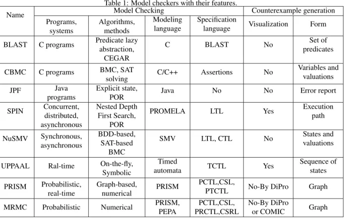
Practically, all successful model checkers are able to output counterexamples in varying formats [38]. In this section, we will try to survey the tools supporting counterexample generation and study their effectiveness. A set of model checkers with their features are presented in Table 1.

Berkeley Lazy Abstraction Software Verification Tool (BLAST) [13] is a software model checking tool for C pro-grams. BLAST has the ability to generate counterexam-ples, and furthermore, it employs CEGAR. BLAST is not just a CEGAR-based model checker, but it can be also used for generating test cases. BLAST shows promising results with safety properties of programs with a medium size.

CBMC [35] is a well-known Bounded Model Checker for AINCI C and C++ programs. CBMC performs symbo-lic execution on the programs and employs a SAT solver in the verification procedure, when the specification is falsi-fied, a counterexample in the form of states with variables valuation leading to these states is rendered to the user.

JavaPathfinder(JPF) [131] is a famous software model checking tool for Java programs. JavaPathfinder is an ef-fective virtual machine-based tool that verifies the program along all the possible executions. Due to its ability to deal with most of JAVA language features, because it runs on byte-code level, JavaPathfinder can generate a detailed re-port on the error in case that the property is violated. Besi-des, the tool gives the ability to generate test cases.

Table 1: Model checkers with their features.

Name Model Checking Counterexample generation

Programs, systems

Algorithms, methods

Modeling language

Specification

language Visualization Form

BLAST C programs Predicate lazy abstraction,

CEGAR

C BLAST No Set of

predicates

CBMC C programs BMC, SAT

solving

C/C++ Assertions No Variables and

valuations

JPF Java

programs

Explicit state,

POR Java No No Error report

SPIN Concurrent, distributed, asynchronous

Nested Depth First Search,

POR

PROMELA LTL Yes Execution

path

NuSMV Synchronous, asynchronous

BDD-based, SAT-based

BMC

SMV LTL, CTL No States and

valuations

UPPAAL Ral-time On-the-fly,

Symbolic

Timed

automata TCTL Yes

Sequence of states

PRISM Probabilistic, real-time

Graph-based,

numerical PRISM

PCTL,CSL,

PTCTL No-By DiPro Graph

MRMC Probabilistic Numerical PRISM,

PEPA

PCTL,CSL, PRCTL,CSRL

No-By DiPro

or COMIC Graph

NuSMV [26] is a symbolic model checker that appeared as an extension of the Binary Decision Diagrams(BDD)-based model checker SMV. NuSMV includes both LTL and CTL for specification analysis, and combines SAT and BDD techniques for the verification. NuSMV can deliver a counterexample in XML format by indicating the states of the trace and the variables with their new values that cause the transitions.

UPPAAL [100] is a verification framework for real-time systems. The systems can be modeled as networks of ti-med automata extended with data types and synchroniza-tion channels, and the properties are specified using a Ti-med CTL(TCTL). UPPAAL can find and generate counte-rexamples in graphical mode as message sequence charts that indicate the events with respect to their order.

PRISM [81] is a probabilistic model checker used for the analysis of systems that exhibit stochastic behavior. The systems are described as DTMCs, CTMCs or MDPs, using guarded command language, and verified against probabi-listic properties expressed in PCTL and CSL, and can be extended with rewards. Another successful probabilistic model checker extended with rewards is the Markov Re-ward Model Checker (MRMC) [94]. MRMC is mainly used for performance and dependability analysis. It takes the models as input files in two formats, in PRISM lan-guage or Performance Evaluation Process Algebra (PEPA). Although both model checkers have shown high effective-ness, they lack a mechanism for generating probabilistic counterexamples. Nevertheless, they have been used by re-cent tools (DiPro [2] and COMICS [90]) for generating and visualizing probabilistic counterexamples.

9

Conclusions and future directions

In this paper we surveyed counterexamples in model checking from different aspects. At the beginning of using model checking, counterexamples have not been treated as a particular subject, but they have been treated as a rela-ted problem to fair cycle detection algorithms, as presenrela-ted in section 3. But recently, the quality of the counterex-amples generated has been treated as a standalone and a fundamental problem. Many works tried to deliver short and indicative counterexamples to be used for debugging purpose. Concerning their structure, tree-like counterex-amples have been proposed for the fragment of ACTL as an alternative for linear counterexamples, however, we see that this approach has not been adopted in model checkers, but instead model checkers are still based on generating simple non-branching counterexamples .

For debugging, we can conclude that approaches that re-quire other successful runs might have some advantages over other methods based on single trace, in way that they compare many good traces to restrict the set of candidate causes. However, these methods take usually much execu-tion time in order to select the appropriate set of traces, and besides, such traces could contain the same diagnostic in-formation. Regardless of the debugging method in use, the challenge of visualizing the error traces and the quality of diagnoses generated to facilitate debugging is still an open issue.

where the presentation of counterexample is different from a work to another, from smallest and indicative set of paths to most critical sub-systems. Despite the notable advance-ment in generating probabilistic counterexamples that led to inventing important tools like DiPro and COMICS, un-fortunately this advancement is still insufficient for debug-ging. Actually, it is more than important to see the techni-ques for counterexample generation and counterexample analysis integrated in probabilistic model checkers to get their benefit. All these techniques act on verification results of probabilistic model checkers like PRISM, so making the approaches of counterexample generation and counterex-amples analysis to be performed during the model checking process itself is still an open problem. This could really have a great impact on probabilistic model checking.

We have also seen the usefulness of counterexamples for other purposes than debugging, like CEGAR and test cases generation. For CEGAR, we have seen different approa-ches for both abstraction and refinement. We have seen that we can benefit from using SAT solvers and theorem provers on the both sides, abstraction and refinement, thus they are very useful for CEGAR. Fast elimination of spu-rious counterexamples is still an active research topic. We also expect to see more works on CEGAR in PMC.

For testing, we have seen that the most useful approaches using model checking are those based on coverage and trap properties. Other approaches for testing like requirement-based analysis and mutation-requirement-based analysis have received smaller attention due to the limitations presented. Cur-rently, coverage-based techniques are widely used in the industry. In the future, we expect to see the proposition of new approaches to enable us to test new emerging sy-stems, which require new transformation mechanisms for enabling trap properties to be verified by model checkers to generate the counterexamples.

We should mention that such techniques can benefit from other techniques. For instance, new efficient CEGAR techniques will not only have an impact on conventional model checking, but on probabilistic model checking as well. We can also see in the future the use of probabilis-tic model checkers like PRISM for testing probabilisprobabilis-tic sy-stems. Since PRISM does not generate counterexamples, any advancement in generating indicative counterexamples could be of benefit for testing probabilistic systems. We can also see that techniques based on counterexamples like CEGAR can directly benefit from any advancement in ge-nerating small and indicative counterexamples in a consi-derable time.

In addition to all of this, we expect to see more works in other domains that adapt model checking techniques just for the seek of getting counterexamples. In previous works we have seen for instance that counterexamples can be mapped to UML sequence diagrams, describing states and events in the original model [51], they can be used to gene-rate attack graphs in networks security [123], in fragmen-tation of services in Service-Based Applications (SBAs) [21], and they have been also used to enforce

synchroni-zability and realisynchroni-zability in distributed services integration [72].

References

[1] Aljazzar, H., Hermanns, H., and Leue, S. Coun-terexamples for timed probabilistic reachability. In FORMATS(2005), LNCS, vol. 3829, Springer, Ber-lin, Heidelberg, pp. 177–195.

[2] Aljazzar, H., Leitner-Fischer, F., Leue, S., and Si-meonov, D. Dipro - a tool for probabilistic coun-terexample generation. In18th International SPIN Workshop(2011), LNCS, vol. 6823, Springer, Ber-lin, Heidelberg, pp. 183–187.

[3] Aljazzar, H., and Leue, S. Extended directed search for probabilistic timed reachability. InFORMATS (2006), LNCS, vol. 4202, Springer, Berlin, Heidel-berg, pp. 33–51.

[4] Aljazzar, H., and Leue, S. Generation of counterex-amples for model checking of markov decision pro-cesses. InInternational Conference on Quantitative Evaluation of Systems (QEST)(2009), pp. 197–206. [5] Aljazzar, H., and Leue, S. Directed explicit state-space search in the generation of counterexamples for stochastic model checking.IEEE Trans. on Soft-ware Engineering 36, 1 (2010), 37–60.

[6] Aljazzar, H., and Leue, S. K*: A heuristic search algorithm for finding the k shortest paths. Artificial Intelligence 175, 18 (2011), 2129 – 2154.

[7] Aloul, F., Ramani, A., Markov, I., and Sakallah, K. Pbs: A backtrack search pseudo boolean solver. In Symposium on the Theory and Applications of Satis-fiability Testing (SAT)(2002), pp. 346–353.

[8] Andres, M. E., DArgenio, P., and van Rossum, P. Significant diagnostic counterexamples in probabi-listic model checking. InHaifa Verification Confe-rence(2008), pp. 129–148.

[9] Aziz, A., Sanwal, K., Singhal, V., and Brayton, R. Model-checking continuous-time markov chains. ACM Transactions on Computational Logic 1, 1 (2000), 162–170.

[10] Baier, C., Haverkort, B., Hermanns, H., and Katoen, J.-P. Model checking algorithms for continuous-time markov chains.IEEE Transactions on Software Engineering 29, 7 (2003), 524–541.