CAS: Recursive Credibility: Using Credibility to Blend Reserve Assumptions

Recursive Credibility: Using Credibility

to Blend Reserve Assumptions

by Marcus M. Yamashiro

ABSTRACT

MCL formulas come so close to the recursive appli-cation of credibility, some questions arise, such as:

1. Would recursive credibility of the CL and XL give more stable results than the MCL?

2. Can recursive credibility be applied to other loss development assumptions?

3. Can recursive credibility be applied to more than two loss development assumptions?

Recursive credibility-weighting of development assumptions can have certain unique advantages. Faced with a limited quantity of data and volatile loss devel-opment history, we often reach for multi variate tools to enhance the predictive power of our models. As a multi-assumptional tool, recursive credibility can help us to reduce the error in our model selection. Not only can it show how much weight to give each model, it can also show us when to do so. For instance, workers compensation loss development may be consistent with CL assumptions in early development ages, gradually switching over to behave more like annuity payments in later ages as indemnity and medical costs become routine, and as a greater percent of remaining claimants have lifelong catastrophic injuries. Recursive credibil-ity can give varying weight over the loss development period to different model assumptions based on these changing drivers of loss development.

Recursive credibility could also have drawbacks, such as the potential instability caused by an iterative process. One approach to mitigating this instability is utilizing the error caused by the credibility weights themselves. To understand why this is, consider the weighted sum, Z × f + (1 − Z) × g of two estimates, f and g, of the same quantity. Measurement error in this weighted sum is caused by error in all three vari-ables, f, g and Z. Often, in determining least squares credibility, only error in f and g are considered.2 _But error in the estimation of the variance and covariance of f and g will result in error in Z as well. Including credibility weight error in a minimization procedure

1. Introduction

A recent contribution to reserving methodologies is the Munich chain ladder (MCL) of Quarg and Mack (2008), which recursively adjusts paid and reported loss development patterns based on the relative size of case reserves. It is designed to reduce the gap between paid and incurred ultimate loss indications. Performed via regression on conditional residuals, this aspect of the MCL is of seminal value to the actuarial commu-nity. Jedlicka (2007) has described multivariate exten-sions of the MCL that demonstrate the flexibility of regression on conditional residuals.

This paper branches off from the MCL in a dif-ferent direction. It may be surprising that the MCL can be interpreted as the recursive weighting of chain ladder (CL) paid and incurred indications ( fP

s→tPi,s,

fI

s→tIi,s) with cross link1 (XL) paid and incurred

indi-cations (I_i,sgP

s→t, Pi,sgIs→t) respectively. For example, a

paid MCL indication, shown to the left of the approx-imation sign in equation (1.1) is approximately the paid CL indication weighted with the Paid XL indi-cation, to the right of the approximation sign in equa-tion (1.1), i.e.:

1 (1.1)

, ,

1 1

, ,

1

P f Q q

P f W I g W

i s s t P

i s s P

s t P

s Q

i s s t P

s t g

i s s t P

s t g

P P

(

)

(

)

(

)

+ − λ σ σ ≈

− +

→ − − →

→ → → →

−

See Appendix A for a proof of equation (1.1).

This interpretation sheds some light on a source of instability in the MCL. Basing paid development on incurred losses and incurred development on paid losses often results in zigzagging indications. If sig-nificant weight happens to be given to this zigzagging indication, it could result in some instability.

In fact, the MCL is not a strict credibility approach. The MCL formulas do not appear to have been designed to weight the CL with the XL, but rather to adjust for correlation between paid and incurred loss develop-ment using regression. Recognizing, however, that the

1_{In a cross link indication, paid losses are developed as a factor times}

incurred losses and incurred losses are developed as a factor times paid losses. See Appendix A.3 for a description of the cross link indication.

2_{For example, Venter (1990) describes least squares credibility in which}

stable with respect to one another, self-correcting after crossing, then converging.

A simulation documented in section 5 shows that this is not an isolated example. Rather, the MCL has occasional volatility problems, while RC( f, g) is sig-nificantly more stable, resulting in paid and incurred indications that converge quite consistently.

The credibility framework described in this paper has two distinct elements. First, it illustrates a means of recursively defining credibility. It builds a framework that borrows its structure from Thomas Mack’s (1994) chain ladder variance estimate. Second, it shows a method for determining credibility that includes cred-ibility weight error. This method relies on a twist on credibility, thinking of it as the relative distance from a straight average. In doing so, zero-sum weights and zero-sum constants are defined. This paper combines those two elements into a single recursive credibility framework. While this paper focuses on the CL and XL assumptions, the framework has the flexibility to be used with other models as well.

Section 2 lays basic groundwork with definitions to be used throughout the paper, including model and submodel notation. Large negative credibility weights are described as motivation for measurement of cred-ibility weight error, and error in credcred-ibility weights is shown to be equivalent to error in zero-sum weights (to be defined). Then, three key credibility assumptions results in a more stable credibility-weighted estimate

than a procedure that does not recognize this source of volatility.

This paper presents a recursive credibility (RC) framework which, when using the CL and XL sub-indications (i.e., RC( f, g)3_{), can often develop} rea-sonable converging paid and incurred indications where the MCL fails. This RC framework borrows part of its structure from Mack’s (1994) well-known chain ladder variance estimate, which structures variance in a manner that can be mirrored by other paid and incurred model pairs, allowing recursive credibility to be used amongst these different model assumptions.

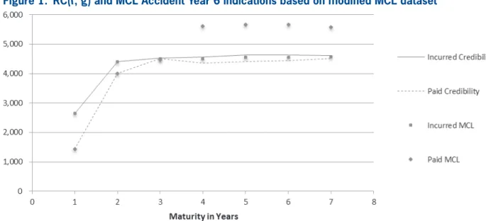
Figure 1 depicts the MCL and RC( f, g) estimates for accident year 6 using the MCL dataset (see Appen dix C), where accident year 4 paid losses have been modified to be 2,286 for development years 1 through 3.

This simple modification of the data results in MCL indications that provide unrealistic loss develop-ment patterns that cross and remain divergent, with paid losses much greater than reported losses. The RC( f, g) incurred and paid indications are more

Figure 1. RC(f, g) and MCL Accident Year 6 indications based on modified MCL dataset

3_{We denote recursive credibility with chain ladder and cross-link}

dent year loss processes is assumed, and definitions of proportionality constants as defined in the MCL paper also apply. Where possible, MCL notational conven-tions have been followed. All n × n paid and incurred development triangles described herein are assumed to have no missing data. The following terminology and general assumptions will be used throughout the paper.

2.1. Paid and incurred loss processes

Let: n ∈ N be the number of accident years, and T be development time (T ⊂ N; T = {1, . . . , n}).

For i = 1, . . . , n, let P_i = (P_i,t)_t∈T and I_i = (I_i,t)_t∈T denote the paid and incurred processes of accident year i, given t development years respectively. The random variables P_i,t and I_i,t denote the paid and incurred losses for accident year i after t develop-ment years.

2.2. Zero-sum weights

Given credibility weights Z_i with i = 1, . . . , n, the set of W_i= Z_i− 1/n will be referred to as “zero-sum weights,” since

Σ

n

i=1 Wi = 0. Consider a

credibility-weighted sum of n indications. Letting I– be the mean of those indications, we can restate the credibility-weighted sum of n indications as the mean indication plus the zero-sum weighted indications, or the mean indication plus the zero-sum weighted deviations from the mean.

(2.1) 1

1

1

I Z I

I W I

I W I I

R

i i i n

i i i n

i i i

n

∑

∑

∑

(

)

( )

( )

=

= +

= + −

=

=

=

Since these zero-sum weights are simply standard credibility weights minus a constant, it is clear that they have the same variance as standard credibility weights. Therefore, determining the variance of zero-sum weights is equivalent to determining the variance of credibility weights. The second line of equation 2.1 will be used as the basis for determining the variance of are made that define a variance of zero-sum weights

as an expression based on a single parameter, coined the zero-sum constant. The parameterization of the zero-sum constant is described in Appendix A.2.

In section 3, each term in Mack’s (2008) recursive variance formula4 _{for the CL is shown to be the sum} of two conditional variance terms. This framework is a general variance structure that can be used with other recursive estimates. In Appendix A.3, the CL and XL are described, and similar recursive vari-ance estimates for the XL are specified as the sum of two conditional variance terms that are analogous to the terms in Mack’s (2008) formula. Proportionality constants as well as conditional covariance terms are also defined.

Section 4 gives an estimate of the variance of a credibility-weighted indication based on two sub-models in a manner that contemplates the variance of the credibility weight itself using Assumptions 1 and 2 from Section 2. Least squares regression is used to determine equations for the two weights. Appen-dix A.4 contains derivations of the variance and cred-ibility equations for two sub-indications.

Section 5 demonstrates how to combine the results of Sections 3 and 4 with calculations for RC based on CL and XL sub-indications—i.e., RC( f, g). It con-tains results of a simulation comparing the MCL with RC( f, g). Then it ends with a comparison of the same methods using over 300 paid and reported grid pairs of industry data.

Section 6 contains concluding remarks, including commentary on strengths and weaknesses of the RC framework, and future research.

2. Loss processes, notation,

and credibility weight error

This paper depends upon and builds on structures and assumptions of the MCL and Mack’s (1994) chain ladder variance equations. Thus, independence of

acci-4_{Mack’s recursive chain ladder variance formula is mathematically}

and the loss type and subscripts denoting the age-to-age values. For instance, σˆ fP

6→7 is the paid CL propor-tionality constant for development from age 6 to 7. Zero-sum constants will be denoted similarly, except with a subscripted W. For example, σˆ_WfP _{denotes the}

zero-sum constant for the paid CL.

2.4. Negative credibility weights

Least squares credibility that contemplates covari-ance of indications can result in negative credibility weights. A question that may arise is “What do neg-ative credibility weights mean?” As an illustration, assume that indication A always deviates from Actual by twice the deviation of indication B. Then

A− Actual = 2(B − Actual). Thus, Actual = 2B +

(−1) A. In this instance, Actual can be determined using solution credibility weights −1 and 2. In gen-eral, for two indications A and B, when the quantities (A − Actual) and (B − Actual) are highly correlated, negative credibility weights can result.

As a second illustration, assume that A histori-cally deviates from Actual by .99 times the deviation of B. Then A − Actual = .99(B − Actual), and Actual =

100A − 99B. Clearly, the parameter error contribution to total estimation error associated with credibility weights of 100 and −99 could be significant.

This parameter error could cause significant distor-tions to least squares credibility-weighted indicadistor-tions. Recognizing error in the credibility weights can help to mitigate these distortions without adding prohibi-tively to the complexity of a credibility framework.

2.5. Zero-sum weight error

In addition to assumptions regarding loss devel-opment, variance and independence, RC depends on the following key assumptions concerning zero-sum weight error.

Assumption 1: Given an RC indication based

on two sub-indications, parameter variance of the zero-sum weights is inversely proportional to the squared difference between the sub-indications.

Appendix A.2 shows that this assumption is based on actual process error patterns.

the credibility-weighted sum of indications. Express-ing credibility in this way will help us to manage the heteroscedasticity problem associated with credibil-ity weight error − credibility weight error grows as dis-tance from the average grows − while still allowing for a simple linear error minimization procedure.

2.3. Model and submodel notation

Since this paper concerns the interrelationship of models, notational conventions used in this paper are stated here for clarity. The letters f and g will refer to the CL and XL models respectively. Loss indi-cations, denoted P and I for paid and case incurred losses respectively, will have subscripts denoting time values, and superscripts denoting the model. Development factors will be denoted by model let-ter, with subscripts denoting age-to-age values and superscripts denoting the loss type. For example, the paid loss chain ladder indication for accident year 3 at maturity 7 is calculated and denoted fP

6→7P3,6f = P3,7f . The term “submodel” refers to a model and related assumptions that is being recursively credibility-weighted with other model assumptions to deter-mine a final best estimate. Conversely, the term “solo model” is used to distinguish a model that is imple-mented as a stand-alone model.

An RC indication will be notated with a capital R superscript. Thus the RC paid loss indication for acci-dent year 3 at maturity 7 is denoted PR

3,7. This means that one or more submodels have been credibility-weighted to give this indication. An RC indication could conceivably refer to a single model credibility indication, in which the single model would always receive full credibility. Thus, RC notation is a gener-alization of independent model notation.

Functions, such as variance or correlation, will be named followed by parentheses. A hat (ˆ) symbol specifies an estimate rather than an actual or theoreti-cal value. For instance, Vaˆr(Pf

3,7) =σˆ2(P3,7f ) is the esti-mate of the variance of the CL paid loss indication for accident year 3, at maturity 7.

weights in the total variance. The large weights that might have been caused by small ratios should not occur.

3. Submodel recursive variance

and covariance expressions

To define least-squares credibility of loss indications recursively, the variance of those indications must also be defined recursively. To see how to accomplish this, consider the following two examples.

First, if I₁ is actual incurred losses at time 1 and a function applied to incurred losses at time 1 is fI

1→2, then the resulting indication, Iˆ₂= fˆI

1→2 (I1). The sec-ond function fI

2→3 is then applied not to actual data, but to the prior indication. That is Iˆ₃ = fˆI

2→3(Iˆ2) = fˆI

2→3( fˆ1→2I (I1)).

As a second example, if I₂ is actual incurred losses at time two, then Iˆ₃= fˆI

2→3(I2).

Even if Iˆ₂ from the first example equals I₂ from the second example, the variance of Iˆ₃ from the first should not equal the variance of Iˆ₃ from the second. The variance of a function performed on a known amount should be different than the variance of the same function performed on an estimate. The vari-ance of Iˆ₃ from the first example must contemplate the error due to fˆI

2→3 as well as the error due to Iˆ2. The variance of Iˆ₃ from the second example only needs to contemplate the error due to fˆI

2→3.

This suggests that the variance of a recursive esti-mate can be considered in two parts, the variance due to error in the function given the prior indication, and the variance due to error in the prior indication given the function. Thomas Mack (2008) has presented his well-known chain ladder variance equations recur-sively, yielding a variance estimate for each recursive loss indication. Thus, the chain ladder ( f ) model can be used as one element in an RC relationship.

The conditional structure of Mack’s (2008) CL vari-ance formula can also serve as a general framework for the variance of some other indications, and this framework facilitates RC relationships. More specifi-cally, each recursive element of Mack’s CL variance formula is the sum of two conditional variance terms,

Assumption 2: Given an RC indication based

on two sub-indications, parameter variance of the zero-sum weights is proportional with

Wˆf 2_Var(If _Ig_).

This assumption forces the error in the credibility weight to equal zero when the weights are equivalent (when zero-sum weights equal zero). The error then increases as the magnitude of the zero-sum weight increases. This assumption also recognizes that error in the weight is proportional to error in the under-lying sub-indications. Appendix A.2 gives a more detailed explanation of this assumption.

Assumptions 1 and 2 Combined: The parameter

variance of a two-indication zero-sum weight is proportional with a scaling expression.

Given the weighted average of two sub-indications {If_{, I}g_{}, based on assumptions 1 and 2, there exists a}

zero-sum constant σI

W, such that:

(2.2)

2 2

2

Var W W Var I I

I I

f W I

f f g

f g

( )

= σ

₍

(

₎

−

)

−

Based on this assumption, the variance of the zero- sum weights (and thus the credibility weights) increases with the magnitude of the zero-sum weights them-selves. This mitigates the possibility of massive cred-ibility weights being output in an error minimization procedure.

Assumption 3: Two-indication zero-sum weights

are independent of sub-indication differences and indication sums as well as the ratios of the sub-indication difference over the sub-sub-indication sum.

This assumption is made to simplify the deriva-tion of the variance of a credibility-weighted sum of indications. It makes zero-sum weights behave as constants in sub-indication covariance expressions. Although this is not a perfect assumption, it is rea-sonable because:

1. The absolute magnitude of indications should clearly be independent of the credibility weights. 2. The impact of the scaled sub-indication difference

KDF, i.e., the variance of the prior indication times the squared development factor:

(3.2)

, ,

2 Var I Di t Var I f

f

s t i s R

s t I

(

→

)

=

( )

→

Reducing the set D_s→t = { fI

s→t, fPs→t} and changing

R to f would make equation (3.2) the second sum-mand from Mack’s recursive variance calculation for incurred losses.

3.3. Mack’s recursive chain ladder

variance term

For incurred and paid losses, the recursive version of Mack’s chain ladder variance expression is thus the sum of the variance given known development factors from development year s to t and the variance given known losses through development year s.

(3.3)

, , ,

, 2

, 2

2

,

2

, 1

Var I Var I D Var I B s

Var I f I

I I

i t f

i t f

s t i t f

i

i s R

s t I

i s R s t

fI

i s R

s t fI

j s j n s

∑

( )

(

)

(

)

( )

( )

= +

= + σ + σ



 _

→

→ → →

= −

(3.4)

, , ,

, 2

, 2

2

,

2

, 1

Var P Var P D Var P B s

Var P f P

P P

i t f

i t f

s t i t f

i

i s R

s t P

i s R s t

fP

i s R

s t fP

j s j n s

∑

( )

(

)

(

)

( )

( )

= +

= + σ + σ



 _

→

→ → →

= −

Converting from the submodel recursive variance for-mulas of equations 3.3 and 3.4 to solo model formu-las by allowing R to equal f, would precisely make these equations Mack’s recursive variance formulas for incurred and paid losses for a single accident year (2008).

In Appendix A.3, CL and XL submodel indica-tions are defined, and recursive variance equaindica-tions are described as the sum of variance given KPL and variance given KDF. Additionally, proportionality con-stants are defined, as well as KPL correlation and KDF covariance for the given submodels.

where the two conditions are the known prior losses (KPL) condition, and the known development factors (KDF) condition. The KPL and KDF conditions will be used throughout the paper for different models, with the same meaning as defined below.

For this framework to remain simple, it will be assumed that volatility given KPL and volatility given KDF are independent of one another across indica-tions, and this will allow the sum of the covariance given KPL and the covariance given KDF to equal the total covariance.

3.1. The known prior losses

(KPL) condition

Being given the set, B_i(s) = {P_i,1, . . . , P_i,s; I_i,1, . . . , I_i,s}, of paid and incurred development for accident year i until the end of development year s, implies that loss development through development year s is known and constant. This condition is key to Mack’s recursive variance calculation, since it allows the variance to be separated into the variance given KPL through age s (expressed as the total expression in equation (3.1)) and the remaining variance, stated next.

(3.1)

, ,

2 2

,

2

, 1

Var I B s I

I I

i t f

i i s R s t

fI

i s R

s t fI

j s j n s

∑

(

( )

)

= σ + σ 

 → → _

= −

Recalling that RC notation is a generalization of inde-pendent model notation, where R is allowed to equal f, equation (3.1) is a summand from Mack’s recursive variance formula for incurred losses.

3.2. The known development factors

(KDF) condition

The variance that remains, excluding the KPL vari-ance is the KDF varivari-ance, described here. Suppose we have three pairs of loss development assumptions f, g, and h. Being given the set D_s→t= {fI

s→t, fPs→t; gIs→t,

gP

s→t; hsI→t, hPs→t} of factors based on these assumptions,

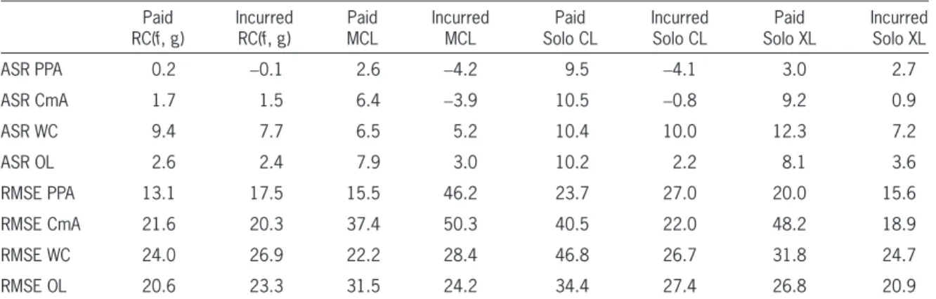
Both sets of conditional covariance terms can be fully expressed using equations (A.23) to (A.27).

We now have all the necessary elements to square a triangle with a recursive credibility indication. Below, the steps are listed sequentially and they are dem-onstrated with a numerical example in the next section. Parameter Steps: We use the data in the upper tri-angular matrix to calculate parameters needed for the sub-indication models and for implementing recursive credibility.

Step P1: We calculate submodel parameters and values associated with the upper triangular matrix.

Step P1a: Development factors (based on volume-weighted averages)

Step P1b: Indications (using equations (A.14), (A.15), (A.18), and (A.19))

Step P1c: Proportionality constants (using equa-tion (A.22))

Step P1d: Variances (using equations (A.16), (A.17), (A.20), and (A.21))

Step P2: We calculate RC parameters associated with the upper triangular matrix.

Step P2a: Correlations given known prior losses (using equations (A.23) and (A.24)).

Step P2b: Zero-sum constants σI

W and σPW (using

equation (A.12)).

Development Steps: We use the values calculated from the upper triangular matrix in Steps P1 and P2 to iteratively add diagonals to the development triangle, “squaring” the triangle.

Step D1: Using parameters from Step P1, we calculate the incurred and paid sub-indications If

i,t, Igi,t, Pi,tf and

Pg

i,t, and the submodel variance terms.

Step D2: Relying on equation (4.3), we use KPL cor-relations from step P2 and KDF covariance terms from equations (A.25) and (A.26) to determine the total covariance of the underlying sub-indications. Step D3: Using equation (4.2) and zero-sum constants

from Step P2, we calculate the zero-sum weights WfI

i,t and WgIi,t (and likewise Wi,tfP and WgPi,t).

Step D4: Using the zero-sum weights calculated in Step D3 and equation (2.1), we calculate the RC indication IR

i,t (and likewise PRi,t).

4. Credibility procedure:

Contemplating error in the weights

By considering the variance of the credibility-weighted sum of two indications (equation (2.1)) and contemplating error in the credibility weights (equa-tion (2.2)) the variance of the credibility-weighted estimate can be determined (equation (4.1)). The der-ivation of this estimate, which depends on Assump-tion 3 that credibility weights are constant in the covariance terms, and Wf I

i,t selected to minimize the

variance, is shown in Appendix A.4.

0.25

0.5

(4.1)

, , , , , ,

, , ,

Var Z I Z I Var I I

Var I Var I W

i t fI

i t f

i t gI

i t g

i t f

i t g

i t g

i t f

i t f I

(

)

(

)

( )

( )

(

)

+ = +

− −

Equation (4.2) is the theoretical zero-sum weight as derived in Appendix A.4.

0.5

(4.2) ,

, , , ,

2

, ,

, ,

2 ₂

, ,

2

2

, ,

W Var I Var I I I

Var I I I I I I

Var I I

i t

fI i t

g

i t f

i t f

i t g

i t f

i t g i t

f i t g

W I

i t f

i t g

W I

i t f

i t g

(

( )

( ) (

)

)

(

)

(

)

(

)

(

)

= − −

− − + σ −

+ σ −

 

 

Following are descriptions of a few final details needed to complete a recursive credibility indication.

First, in addition to individual loss indications, variance terms, and a zero-sum parameter, equations (4.1) and (4.2) contain the expressions Var(If

i,t− Ii,tg)

and Var(If

i,t+ Igi,t), which can be expanded to Var(Ii,tf) +

Var(Ig

i,t) − 2Cov(Ii,tf, Igi,t) and Var(Ii,tf) + Var(Ii,tg) +

2Cov(If

i,t, Ii,tg) respectively.

Next, by the assumption from Section 3 that vola-tility given KPL and volavola-tility given KDF are inde-pendent of one another across sub-indications, the covariance term can be expressed as follows:

, , ,

(4.3)

, , , , , ,

Cov I Ii t Cov I I D Cov I I B s

f i t g

i t f

i t g

s t i t f

i t g

i

ˆ 2074 2284 4494

2024 2232 4416 1.021

4 5

,5

,4

f P

P

P _i i i i

∑

∑

= = + +

+ + =

→

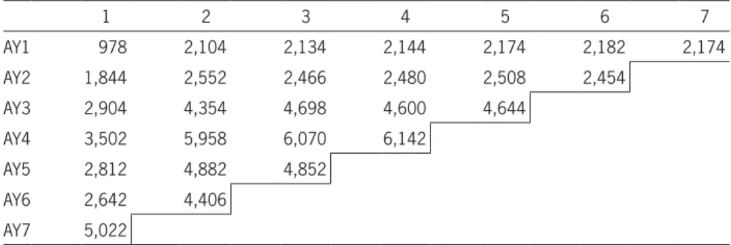
Step P1b: Indications (using equations (A.14), (A.15), (A.18), and (A.19))

Tables C.1, C.2, C.3, and C.4 contain upper triangu-lar matrix indications, calculated by multiplying losses from Tables B.1 and B.2 by development factors from Table 1. Each indication in the upper triangular matrix is calculated as the actual loss times the development factor. For example:

ˆ _{ˆ .945 4882 4613}

5,3 2 3 5,2

Pg=g IP = × =

→

Step P1c: Proportionality constants (using equa-tion (A.22))

Based on equation (A.22), the proportionality con-stant for each submodel by loss development maturity is the square root of the sum of the squared, scaled loss indication residuals divided by their degrees of freedom (where the residuals are scaled by prior his-torical losses). As an example, we use the indications from Table C.4 and the losses from Table B.1 to illus-trate the incurred XL proportionality constant from age 3 to 4.

ˆ ˆ

7 3 1

2144 2146 2134

2480 2355 2466 4600 4631

4698

6142 6234 6070

7 3 1 1.63

3 4

,4 ,4 2

,3 1

4

2 2

2 2

I I I

gI i i

g i i

∑

(

)

( ) ( )

( ) ( )

σ = −

− −

=

− ₊ −

+ − + −



   



   

− − =

→

=

The paid and incurred CL and XL proportionality constants by age are listed in Table 2.

0.5 (4.4)

, , , , , , ,

Ii t I I I W I W

R

i t f

i t g

i t f

i t f I

i t g

i t gI

(

)

= + + +

0.5 (4.5)

, , , , , , ,

Pi t P P P W P W

R

i t f

i t g

i t f

i t fP

i t g

i t gP

(

)

= + + +

Step D5: Using equation (4.1) and the weights calcu-lated in Step D3, we calculate the variance of the RC indication at time t, Var(IR

i,t) (and likewise Var(PRi,t)).

5. Numerical example

To demonstrate recursive credibility with a numer-ical example, we will first calculate parameters, and then two years of development for the fifth accident year of the MCL dataset (tables B.1 and B.2). We will follow the (P)arameter and (D)evelopment steps out-lined above. Then we will compare RC( f, g) paid and incurred loss development patterns to those implied by the CL and XL models.

At the end of this section, some statistics are doc-umented from a simulation directly comparing the MCL with RC( f, g). These statistics demonstrate that the RC( f, g) indications are more stable than the MCL derived indications.

5.1. Parameter steps

Step P1: We calculate submodel parameters and indi-cations based on the upper triangular matrix Step P1a: Development factors (based on

volume-weighted averages)

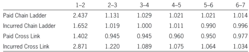
Table 1 contains all-year weighted average devel-opment factors, calculated using historical data from tables B.1 and B.2. As an example, the 3-4 factor for the Paid XL and the 4-5 factor for the Paid CL are cal-culated as follows:

ˆ 2024 2232 4416 5850

2134 2466 4698 6070 0.945

3 4

,4

,3

g P

I

P _i i i i

∑

∑

= = + + +

+ + + =

→

Table 1. All-year weighted average development factors

1–2 2–3 3–4 4–5 5–6 6–7

Paid Chain Ladder 2.437 1.131 1.029 1.021 1.021 1.014

Incurred Chain Ladder 1.652 1.019 1.000 1.011 0.990 0.996

Paid Cross Link 1.402 0.945 0.945 0.960 0.950 0.977

A conditional residual (defined by equation (A.23)) is a scaled residual divided by the proportional-ity constant (where the scaling term is the square root of the prior age losses). Thus, a paid XL con-ditional residual for accident year 2 at age 4 is

(

2232 2330−

)

_{= −}

2162 1.52 1.39. Based on the

condi-tional residuals shown below in Tables 3 and 4, we can now calculate the correlation given KPL as

ˆ ,

1.27 1.24 0.14 0.45

. . . _{.18 1.66 .57 .97}

6 5 2

0.0765 P P KPLf g

(

)

( )( ) ( )( )

( )( ) ( )( )

( )( )

ρ =

+ − −

+ + +



 

= −

Step P1d: Variances (using equations (A.16), (A.17), (A.20), and (A.21))

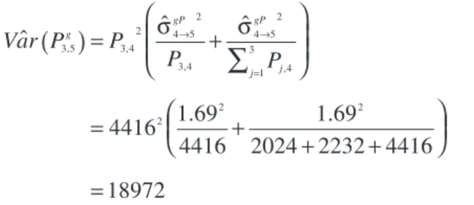
Variances for the upper triangular matrix of indica-tions are calculated using data from Tables B.1 and B.2, and proportionality constants from Table 2. Since each entry in the upper triangular matrix of indica-tions is calculated using only historical losses multi-plied by a single factor, the KDF variance terms are always equal to zero, which simplifies all the upper triangular matrix variance terms to be only KPL vari-ance terms. For example:

Var P P

P P

g

gP gP

j j

∑

( )

= σ + σ 

 _

= +

+ +

 

 _

=

→ →

=

ˆ ˆ ˆ

4416 1.69

4416

1.69

2024 2232 4416

18972 3,5 3,4

2 4 5 2

3,4

4 5 2

,4 1 3

2

2 2

The upper triangular matrix variances are presented in Tables C.5, C.6, C.7, and C.8.

Step P2: We calculate RC parameters associated with the upper triangular matrix.

In Step P1, we calculated values associated with each of the individual submodels. In Step P2, we cal-culate parameters necessary to combine the informa-tion from the submodels.

Step P2a: Correlation given known prior losses (using equations (A.23) and (A.24)).

The correlation between loss indications given KPL is calculated across the upper triangular matrix (using equation (A.24)) as the sum of the product of conditional residual pairs divided by the degrees of freedom. Thus, to calculate the correlation given KPL, we first need conditional residuals.

Table 2. Proportionality constants

1 to 2 2 to 3 3 to 4 4 to 5 5 to 6 6 to 7*

Paid Chain Ladder 13.46 3.67 0.48 0.21 0.48 0.24

Incurred Chain Ladder 9.73 2.54 1.00 0.12 0.86 0.43

Paid Cross Link 14.19 3.13 1.52 1.69 1.08 0.54

Incurred Cross Link 9.53 3.36 1.63 1.88 0.71 0.36

*Half of the prior age proportionality constant is used here, but other assumptions could be appropriate

Table 3. Paid CL conditional residuals

2 3 4 5 6

AY1 1.24 −0.45 −0.18 0.85 −0.72

AY2 −0.41 −0.26 0.29 0.57 0.69

AY3 0.63 0.00 1.25 −0.98

AY4 −0.43 −0.98 −1.15

AY5 −1.33 1.66

AY6 0.97

Table 4. Paid XL conditional residuals

2 3 4 5 6

AY1 1.27 −0.14 0.11 0.22 0.72

AY2 −1.53 −1.81 −1.39 −1.20 −0.69

AY3 −0.59 0.72 −0.24 0.71

AY4 0.56 0.41 1.00

AY5 −0.27 0.18

ˆ ˆ

ˆ ˆ 0.5

0.5 ˆ_ˆ

ˆ

3778 3944

4552 3944 0.5

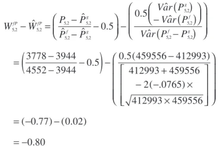
0.5 459556 412993 412993 459556 2 .0765 412993 459556 0.77 0.02 0.80 5,2 5,2 5,2 5,2 5,2 5,2 5,2 5,2 5,2 5,2

W W P P

P P

Var P Var P

Var P P

fP fP g f g g f f g

(

)

( )

( )

(

)

( ) ( ) ( ) ( ) − = − − −    − −    −         = − − − − − + − − × ×                     = − − = −

To scale the paid zero-sum residual, the scaling factor for accident year 5 at time 2 is

ˆ

ˆ ˆ

0.52 412993 0.48 459556

2 .0765 0.52 0.48) 412993 459556

4552 3944

0.7370

5,2 5,2 5,2 5,2

5,2 5,2 2

2 2

2

Var Z P Z P

P P

f P f gP g f g

(

)

(

)

( ) ( ) ( ) ( )( ) ( )( ) ( ) + − = + + −     − =

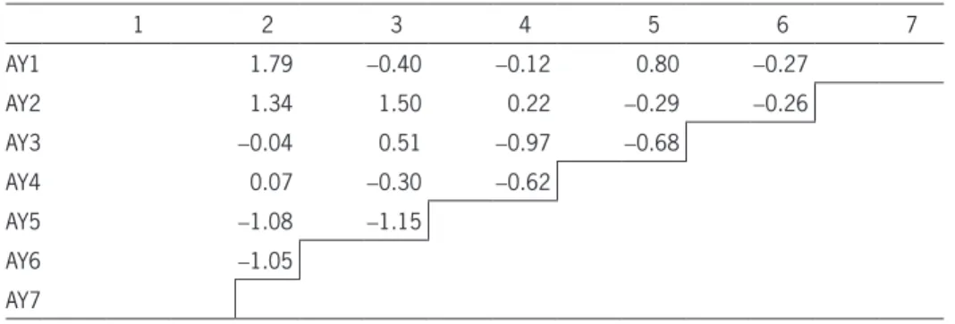
Thus, the scaled residual is −0.80 / 0.7370 =−1.08. Table 7 contains for the upper triangular matrix, the set of scaled residuals for the paid CL (which are the negative scaled residuals for the Paid XL).

Based on these paid scaled zero-sum residuals, the paid zero-sum constant is calculated based on equa-tion (A.12) as follows:

W W P P

W P P

n n n n

W P i t f P i t f P i t f i t g i t f P i t f i t g t n i i n

∑

∑

(

) (

)

(

)

( ) ( )

(

)(

) (

)(

)

(

)(

)

( ) ( ) ( ) σ = − −

+ σ σ

      − −    + −  = + − + + − + − × × = = + − = − ˆ

ˆ ˆ ˆ

0.25 ˆ ˆ ˆ

1 2

2

1 2

2

1.79 0.40 . . . 1.15 1.05

6 5 2 8 5 2

0.2167 , , 2 , , 2 , 2 , , 2 1 1 1

2 2 2 2

The incurred zero-sum constant can be likewise calcu-lated to be σˆI

W= 0.2015. The purpose of these

param-eters is to serve as a measure of the uncertainty in the An incurred CL conditional residual for accident

year 5 at age 3 is

(

4852 4973−

)

= −

4882 2.54 0.68. Based

on the conditional residuals shown below in Tables 5 and 6, we can calculate the correlation given KPL as ρˆ(If_{, I}g| _KPL) = _0.0355.

Step P2b: Zero-sum constants (using equation (A.12)) Zero-sum constants can be thought of as a portion of the standardized deviation of zero-sum weights from actual weights that would produce a correct solu-tion (zero-sum residuals). To calculate a single paid zero-sum residual, take the difference between a solu-tion weight WfP

i,t such that (Wf Pi,t− 0.5) Pˆi,tf + (Wi,tfP+ 0.5)

Pˆg

i,t= Pi,t, calculated W

P P

P P

i t

fP i t i t g i t f i t g = − − − ˆ

ˆ ˆ 0.5

,

, ,

, ,

and an

esti-mated weight, based on equation (4.2), and setting the zero-sum constant equal to zero, calculated

W Var P Var P

Var P P

i t

fP i t g i t f i t f i t g

( )

( )

(

)

(

)

= − −

ˆ 0.5 ˆ ˆ

ˆ .

,

, ,

, ,

Using paid

indica-tions from Tables C.1 and C.2, paid variances from Tables C.5 and C.6 and the KPL correlation calcu-lated in Step P2a, the zero-sum weight residual for accident year 5, at time 2 is calculated.

Table 5. Inc’d CL conditional residuals

2 3 4 5 6

AY1 1.61 −0.08 0.22 1.13 0.73

AY2 −1.18 −1.04 0.29 0.10 −0.68

AY3 −0.85 1.57 −1.42 −0.84

AY4 0.30 0.00 0.93

AY5 0.46 −0.68

AY6 0.08

Table 6. Inc’d XL conditional residuals

2 3 4 5 6

AY1 1.51 −0.43 −0.02 −0.03 −0.73

AY2 0.16 0.53 1.55 1.15 0.68

AY3 0.59 0.52 −0.28 −0.82

AY4 −1.07 −1.48 −0.73

AY5 −0.95 1.04

Var P P

P P

g

gP gP

j j

∑

( )

= σ + σ 

 _

= +

+ + +

 

 _

=

→ →

=

ˆ ˆ ˆ

4648 1.52

4648

1.52

1970 2162 4252 5724

14208 5,4 5,3

2 3 4 2

5,3

3 4 2

, 3 1 4

2

2 2

Var P P

P P

f

fP fP

j j

∑

( )

= σ + σ 

 _

= +

+ + +

 

 _

=

→ →

=

ˆ ˆ ˆ

4648 0.48

4648

0.48

1970 2162 4252 5724

1435 5,4 5,3

2 3 4 2

5,3

3 4 2

, 3 1 3

2

2 2

Var I I

I I

g

gI gI

j j

∑

( )

= σ + σ 

 _

= +

+ + +

 

 _

=

→ →

=

ˆ ˆ ˆ

4852 1.63

4852

1.63

2134 2466 4698 6070

16965 5,4 5,3

2 _{3 4} 2

5,3

3 4 2

, 3 1 4

2

2 2

Var I I

I I

f

fI fI

j j

∑

( )

= σ + σ 

 _

= +

+ + +

 

 _

=

→ →

=

ˆ ˆ ˆ

4852 1.00

4852

1.00

2134 2466 4698 6070

6436 5,4 5,3

2 3 4 2

5,3

3 4 2

, 3 1 3

2

2 2

These submodel variances can be found on Tables C.5, C.6, C.7, and C.8.

credibility weights due to the magnitude of the weight itself, which will help to mitigate error due to unrea-sonably large weights.

We have completed the initial parameter steps of the RC framework. Steps 3 through 9 are recursive development steps, which we will calculate for acci-dent year 5.

5.2. Development steps

Step D1 (1st new diagonal): We calculate submodel indications and submodel variance terms

For the first new diagonal, we use historical losses from Tables B.1 and B.2 and development factors from Table 1.

ˆ _{ˆ .945 4852 4585,}

ˆ ˆ _{1.029 4648 4784}

5,4 3 4 5,3

5,4 3 4 5,3

P g I

P f P

g P

f P

= = × =

= = × =

→

→

ˆ _{ˆ 1.089 4648 5062,}

ˆ ˆ _{1.000 4852 4851}

5,4 3 4 5,3

5,4 3 4 5,3

I g P

I f I

g I

f I

= = × =

= = × =

→

→

These submodels can be found on Tables C.1, C.2, C.3, and C.4.

To calculate the submodel variance terms for the first new diagonal, since the prior diagonal is actual historical losses, equations (A.16), (A.17), (A.20) and (A.21) can be simplified. The variance given KDF is equal to zero, and we use historical losses from Tables B.1 and B.2 and proportionality constants from Table 2.

Table 7. Paid CL (–XL) scaled zero-sum residuals

1 2 3 4 5 6 7

AY1 1.79 −0.40 −0.12 0.80 −0.27

AY2 1.34 1.50 0.22 −0.29 −0.26

AY3 −0.04 0.51 −0.97 −0.68

AY4 0.07 −0.30 −0.62

AY5 −1.08 −1.15

AY6 −1.05

For incurred indications, the zero-sum weight is cal-culated as follows:

W Var I Var I I I

Var I I I I I I

Var I I

W

fI

g f f g

f g

f g W

I f g

W

I f g

gI

(

)

(

)

(

)

(

)

(

( )

( )

)

(

)

(

)

( )( ) ( ) ( ) ( ) ( ) = − −

− − + σ −

+ σ −

      = − − + − × − + − + _ + − _                       = = −

ˆ 0.5 ˆ ˆ ˆ ˆ

ˆ ˆ ˆ ˆ ˆ ˆ

ˆ ˆ

0.5 6436 16965 4851 5062 16965 6436 2 .0355 16965 6436

4851 5062 .2015 4851 5062

.2015 16965 6436 2 .0355

16965 6436

0.219 ˆ

5,4

5,4 5,4 5,4 5,4

2 5,4 5,4 5,4 5,4 2 2 5,4 5,4 2 2 5,4 5,4 2

2 2 2

2

5,4

These zero-sum weights can be found on Tables D.1 and D.2.

Step D4 (1st new diagonal): We calculate the RC indications

Using equation (2.1), the submodel indications from Step D1 and the zero-sum weights calculated in Step D3, we calculate the RC indications IˆR

i,t (and

likewise PˆR

i,t) at time t.

IR I I W I W I

f g

f I f gI g

= + + +

= + + −

=

ˆ ˆ ˆ

2 ˆ ˆ ˆ ˆ

4851 5062

2 0.219(4851) 0.219(5062)

4911 5,4

5,4 5,4

5,4 5,4 5,4 5,4

PR P P W P W P

f g

f P f gP g

(

)

(

)

= + + +

= + + −

=

ˆ ˆ ˆ

2 ˆ ˆ ˆ ˆ

4784 4585

2 0.367 4784 0.367 4585

4758 5,4

5,4 5,4

5,4 5,4 5,4 5,4

These RC indications can be found on Tables D.3 and D.4.

Step D2 (1st new diagonal): We calculate the total covariance of the underlying indications

For the first new diagonal, since variance given KDF is equal to zero, the total covariance is equal to covariance given KPL. The correlation given KPL was calculated in step P2, and the submodel variance terms were calculated in step D1.

ˆ ,

ˆ , ˆ 3 ˆ 3

0.0765 14208 1435 346

5,4 5,4

5,4 5 5,4 5

Cov P P

P P KPL P B P B

g f

f g g f

(

)

(

) (

( )

) (

( )

)

= ρ σ σ

= − = −

ˆ ,

ˆ , ˆ 3 ˆ 3

0.0355 16965 6436 371

5,4 5,4

5,4 5 5,4 5

Cov I I

I I KPL I B I B

g f

f g g f

(

)

(

) (

( )

) (

( )

)

= ρ σ σ

= =

Step D3 (1st new diagonal): We calculate the zero-sum weights

Using equation (4.2), we calculate the zero-sum weights WˆfI

i,t and WˆgIi,t (and likewise WˆfPi,t and WˆgPi,t). We

utilize the zero-sum constants from Step P2b, the sub-model indications and subsub-model variance terms from Step D1 and the covariance terms from Step D2. For paid indications, the zero-sum weight is calculated as follows:

W Var P Var P P P

Var P P P P P P

Var P P

W

fP

g f f g

f g

f g W

P f g

W

P f g

gP

(

)

(

)

(

)

(

)

(

( )

( )

)

(

)

(

)

( )( ) ( ) ( ) ( ) = − −

− − + σ −

+ σ −

   _ = − − + − − × − + − + _ + − − _                       = = −

ˆ 0.5 ˆ ˆ ˆ ˆ

ˆ ˆ ˆ ˆ ˆ ˆ

ˆ ˆ

0.5 14208 1435 4784 4585 1435 14208 2 .0765 1435 14208

4784 4585 .2167 4784 4585

.2167 1435 14208 2( .0765)

1435 14208

0.367 ˆ

5,4

5,4 5,4 5,4 5,4

2 5,4 5,4 5,4 5,4 2 ₂ 5,4 5,4 2 2 5,4 5,4 2

2 2 2

2

tors and proportionality constants come from Step P1, the RC indication and variance come from Steps D4 and D5, and historical losses come from Tables B.1 and B.2.

∑

( )

(

)

(

)

( )

( ) ( ) = +

= + σ + σ

   = + + + +    = + = → → → → =

Var I Var I D Var I B

Var I f I

I I

f f f

R I R fI

R

fI

j j

ˆ ˆ ˆ 4

ˆ ˆ ˆ ˆ

ˆ

ˆ

4883 1.011 4911 .12

4911

.12

2144 2480 4600

4992 109 5100

5,5 5,5 4 5 5,5 5

5,4 4 5 2

5,4 2 4 5

2 5,4 4 5 2 ,4 1 3 2 2 2 2

∑

( )

(

)

(

)

( )

( ) ( ) = +

= + σ + σ

   = + + + +    = + = → → → → =

Var P Var P D Var P B

Var P f P

P P

f f f

R P R fP

R

fP

j j

ˆ ˆ ˆ 4

ˆ ˆ ˆ ˆ

ˆ

ˆ

1396 1.021 4758 .21

4758

.21

2024 2232 4416

1455 325 1780

5,5 5,5 4 5 5,5 5

5,4 4 5 2

5,4 2 _{4 5}

2 5,4 4 5 2 ,4 1 3 2 2 2 2

∑

( )

(

)

(

)

( )

( ) ( ) = +

= + σ + σ

   = + + + +    = + = → → → → =

Var I Var I D Var I B

Var P g I

I I

g g g

R I R gI

R

gI

j j

ˆ ˆ ˆ 4

ˆ ˆ ˆ ˆ

ˆ

ˆ

1396 1.075 4911 1.88

4911

1.88

2144 2480 4600

1615 26625 28240

5,5 5,5 4 5 5,5 5

5,4 4 5 2

5,4 2 4 5

2 5,4 4 5 2 ,4 1 3 2 2 2 2

∑

( )

(

)

(

)

( )

( ) ( ) = +

= + σ + σ

   = + + + +    = + = → → → → =

Var P Var P D Var P B

Var I g P

P P

g g g

R P R gP

R

gP

j j

ˆ ˆ ˆ 4

ˆ ˆ ˆ ˆ

ˆ

ˆ

4883 .960 4758 1.69

4758

1.69

2024 2232 4416

4497 20974 25472

5,5 5,5 4 5 5,5 5

5,4 4 5 2

5,4 2 _{4 5}

2 5,4 4 5 2 ,4 1 3 2 2 2 2

These submodel variances can be found on Tables C.5, C.6, C.7, and C.8.

Step D5 (1st new diagonal): We calculate the variance of the RC indications

Using equation (A.34), the submodel variance from Step D1, the covariance terms from Step D2, and the zero-sum weights from Step D3, we calculate the RC variance.

Var Z I Z I

Var I I Var I Var I W

fI f gI g

f g g f f I

(

)

(

)

(

)

(

( )

( )

)

(

)

(

)(

)

+ = + − − = + + − − = ˆ

0.25 ˆ 0.5 ˆ ˆ ˆ

0.25 6436 16965 2 .0355 6436 16965

0.5 16965 6436 0.219

4883

5.4 5.4 5.4 5.4

5.4 5.4 5.4 5.4 5.4

Var Z P Z P

Var P P Var P Var P W

fP f gP g

f g g f fP

(

)

(

)

(

)

(

)

( )

( )

( ) ( )( ) + = + − − = + + − − − = ˆ

0.25 ˆ 0.5 ˆ ˆ ˆ

0.25 1435 14208 2 .0765 1435 14208 0.5 14208 1435 0.367

1396

5.4 5.4 5.4 5.4

5.4 5.4 5.4 5.4 5.4

These RC variances can be found on Tables D.5 and D.6.

Step D1 (2nd iteration): We calculate submodel indi-cations and submodel variance terms

To derive submodel indications for the 2nd new diagonal, we use development factors from Table 1, and instead of historical data, we start with indications from Step D4 (first new diagonal).

ˆ _ˆ ˆ _{.960 4911 4713,}

ˆ ˆ ˆ _{1.021 4758 4857}

5,5 4 5 5,4

5,5 4 5 5,4

P g I

P f P

g P R

f P R

= = × =

= = × =

→

→

ˆ _ˆ ˆ _{1.075 4758 5117,}

ˆ ˆ ˆ _{1.011 4911 4965}

5,5 4 5 5,4

5,5 4 5 5,4

I g P

I f I

g I R

f I R

= = × =

= = × =

→

→

These sub-indications can be found on sub-indication Tables C.1, C.2, C.3 and C.4.

fac-For incurred indications, the zero-sum weight is calculated as follows:

W Var I Var I I I

Var I I I I

Var I I

W

fI

g f f g

f g

f g

W I

W

I f g

gI

(

)

₍

₎

(

)

(

) (

)

(

)

( )

( )

(

)

(

)

(

)

(

)(

)

(

)

= − −

− − + σ

+ σ −

    = − − + − × − + + _{− ×}+       = = −

ˆ 0.5 ˆ ˆ ˆ ˆ

ˆ ˆ ˆ ˆ 1 ˆ

ˆ ˆ

0.5 28240 5100 4965 5117

5100 28240 2 2190

4965 5117 1 .2015 .2015 5100 28240_{2 2190}

0.366 ˆ

5,5

5,5 5,5 5,5 5,5

2 5,5 5,5 5,5 5,5 2 2 2 5,5 5,5 2 2 2 2 5,5

These zero-sum weights can be found on Tables D.1 and D.2.

Step D4 (2nd iteration): We calculate the RC indications

Using equation (2.1), the indications from Step D1, and the zero-sum weights calculated in Step D3, we calculate the RC indications IˆR

i,t (and likewise PˆRi,t).

IR I I W I W I

f g

fI f gI g

= + + +

= + + −

=

ˆ ˆ ˆ

2 ˆ ˆ ˆ ˆ

4965 5117

2 0.366(4965) 0.366(5117)

4985 5,5

5,5 5,5

5,5 5,5 5,5 5,5

PR P P W P W P

f g

fP f gP g

( ) ( )

= + + +

= + + −

=

ˆ ˆ ˆ

2 ˆ ˆ ˆ ˆ

4857 4713

2 0.452 4857 0.452 4713

4850 5,5

5,5 5,5

5,5 5,5 5,5 5,5

These RC Indications can be found on Tables D.3 and D.4.

Step D5 (2nd iteration): We calculate the variance of the RC indications

Using equation (A.34), the submodel variance from Step D1, the covariance terms from Step D2 and the zero-sum weights from Step D3, we calculate the RC variance.

Step D2 (2nd iteration): We calculate the total covari-ance of the underlying indications

For the 2nd new diagonal, we rely on equation (4.3), applying correlations from step P2 and equation (A.27) and covariance terms from equations (A.25) and (A.26) to determine the total covariance of the under-lying submodels.

ˆ ,

ˆ , ˆ ˆ ˆ ˆ

ˆ , ˆ 4 ˆ 4

0.75 4883 .960 1396 1.021

0.0765 20974 325 1719 5,5 5,5

5,4 4 5 5,4 4 5

5,5 5 5,5 5

Cov P P

P I I g P f

P P KPL P B P B

g f

R R R P R P

f g g f

(

)

(

) ( )

( )

(

) (

( )

) (

( )

)

(

)

(

)

= ρ σ σ

+ ρ σ σ

=

− =

→ →

ˆ ,

ˆ , ˆ ˆ ˆ ˆ

ˆ , ˆ 4 ˆ 4

0.75 1396 1.075 4883 1.011

0.0355 26625 109 2190 5,5 5,5

5,4 4 5 5,4 4 5

5,5 5 5,5 5

Cov I I

P I P g I f

I I KPL I B I B

g f

R R R I R I

f g g f

(

)

(

) ( )

( )

(

) (

( )

) (

( )

)

(

)

(

)

= ρ σ σ

+ ρ σ σ

=

+ =

→ →

Step D3 (2nd iteration): We calculate the zero-sum weights

Using equation (4.2), we calculate the zero-sum weights WˆfI

i,t and Wˆi,tgI (and likewise WˆfPi,t and WˆgPi,t). We

utilize the zero-sum constants from Step P2b, the sub-model indications and the subsub-model variance terms from Step D1, and the covariance terms calculated as in Step D2. For paid indications, the zero-sum weight is calculated as follows:

W Var P Var P P P

Var P P P P

Var P P

W

fP

g f f g

f g

f g

W P

W

P f g

gP

(

)

₍

₎

(

)

(

)

(

)

( )

( )

(

)

(

)

₍

₎

(

)

(

)(

)

(

)

= − −

− − + σ

+ σ −

    = − − + − × − + + _{− ×}+       = = −

ˆ 0.5 ˆ ˆ ˆ ˆ

ˆ ˆ ˆ 1 ˆ

ˆ ˆ

0.5 25472 1780 4857 4713

1780 25472 2 1719

4857 4713 1 .2167 .2167 1780 25472_{2 1719}

0.452 ˆ

5,5

5,5 5,5 5,5 5,5

2

for a definition of a solo model) of the CL and XL for Accident Year 7.

Incurred and paid XL indications crisscross with neither indication converging. On the other hand, the incurred and paid CL indications do not converge but appear separately asymptotic, with the paid well below the incurred indication. The incurred and paid RC indications converge between the indications, as would be expected.

Figure 3 illustrates how the incurred CL and XL submodels give very similar indications after the first indication at age 2. This is because the age 3 CL sub-model indication is calculated by multiplying the RC losses at age 2 by the CL factor, and the age 3 XL submodel indication is likewise calculated based on RC losses at age 2. Thus, the maturity 3 indications for both submodels begin from a single pair of RC indications, rather than two pairs of indications—a CL pair and a XL pair.

This practice is consistent with the KPL assump-tion, i.e., that prior to application of a development factor, loss development up until that point is known. Rather than using a submodel’s prior indication as the input for the next loss indication, the RC indication is assumed to be more accurate, thus the next matu-rity’s loss development assumptions apply to the more accurate intermediate indication rather than divergent indications.

Var Z I Z I

Var I I

Var I Var I W

fI f gI g

f g

g f fI

(

)

(

)

( )

( )

(

)

(

)

(

)

( )

+

= +

− −

= + + ×

− −

=

ˆ

0.25 ˆ

0.5 ˆ ˆ ˆ

0.25 5100 28240 2 2190

0.5 28240 5100 0.366

5196

5,5 5,5 5,5 5,5

5,5 5,5

5,5 5,5 5,5

Var Z P Z P

Var P P

Var P Var P W

fP f gP g

f g

g f fP

(

)

(

)

( )

( )

(

)

(

)

(

)

( )

+

= +

− −

= + + ×

− −

=

ˆ

0.25 ˆ

0.5 ˆ ˆ ˆ

0.25 1780 25472 2 1719

0.5 25472 1780 0.452

2320

5,5 5,5 5,5 5,5

5,5 5,5

5,5 5,5 5,5

These RC variances can be found on Tables D.5 and D.6.

5.3. Final RC indications with

CL and XL submodels

Figure 2 shows how the RC( f, g) paid and incurred indications compare to the solo versions (see section 2

prior diagonals of the triangle, based on the implied mu and sigma of actual development ratios by age. 3. Ratios of incremental paid losses as a percentage

of hindsight case reserves5 _{were assumed to be} nor-mally distributed with mean and standard deviation of the actual ratios by age.

a. This amount was capped at 0 and 1.

b. An additional cap of the minimum future incurred loss was set so that historical paid losses would never decrease.

c. These assumptions were used to fill out the paid loss triangle starting from the earliest calendar period (the upper left corner of the triangle). Table 8 contains RC indications as well as the CL

and XL solo indications at age 7 by accident year.

5.4. Comparison of the performance

of the MCL with the RC(

f, g

)

Recalling that the MCL is the weighted sum of the CL and XL indications, an interesting comparison would then be between the MCL and the RC( f, g) indi-cations. To do this comparison, a 10,000 iteration sim-ulation was performed that changed values within the MCL dataset based on the actual triangle distribution.

The simulation design was as follows:

1. The final paid and incurred diagonal of the MCL dataset was unchanged in each iteration.

2. Incurred loss development ratios were assumed to be normally distributed, and used to back into the

Figure 3. RC(f, g) with CL and XL sub-indications for Accident Year 7

Table 8. RC(f, g), and CL and XL solo indications at age 7

Accident Year Paid RC Incurred RC Paid CL Incurred CL Paid XL Incurred XL

1 2,131 2,174 2,131 2,174 2,131 2,174

2 2,385 2,435 2,380 2,445 2,397 2,428

3 4,610 4,701 4,652 4,582 4,669 4,565

4 6,126 6,250 6,182 6,126 6,124 6,184

5 4,976 5,075 5,056 4,839 5,047 4,847

6 4,620 4,714 4,934 4,476 4,521 4,885

7 7,180 7,325 6,128 8,429 6,020 8,580

Total 32,028 32,674 31,463 33,071 30,909 33,664

5_{The hindsight case reserve at time n + 1 equals incurred losses at time}

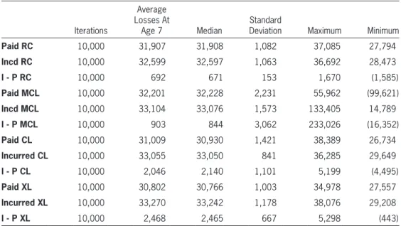
Note that RC( f, g) behaves as desired with incurred and paid averages, minimums and maximums being relatively near those of the CL and XL indications. Furthermore, the average incurred minus paid losses are only $692 with a low standard deviation of only $153. By comparison, the MCL paid, incurred, and incurred minus paid standard deviations are all the highest of the group, with the incurred minus paid stan-dard deviation being higher than either the incurred or the paid standard deviation. The minimums and maxi-mum demonstrate that additional volatility.

Within the simulation detail (not shown) many MCL indications are very close to the RC( f, g) indi-cations, but a number of them also displayed vola-tility. This limited robustness can limit the MCL’s usefulness with volatile data.

Another point to notice is that the median MCL indications are higher than those of RC( f, g). The average of the median paid and incurred MCL of 32,652 is clearly closer to the CL incurred indica-tion of 33,050 than the paid indicaindica-tion of 30,930. The average of the median paid and incurred RC( f, g) indications is 32,252, closer to the average of the median paid and incurred CL indications of 31,990. Whether this indicates systematic bias of one or both of the indications has not been determined. However, this difference should be duly noted in The intention was to build triangles that have

“normal” development (paid losses monotonically increase, and incurred losses are non-negative) that could have led to the final diagonal on the MCL tri-angle from the same set of exposures. Ten thousand such “normal” triangles were generated, using Excel’s random number generator. Eight values were recorded for each iteration, one for each paid and incurred indi-cation for each of the RC( f, g), the MCL, the solo CL and the solo XL models. All the statistics in Table 9 refer to these values.

For both the RC( f, g) and MCL indications, which depend on non-zero proportionality constants, when a constant was calculated as zero, half the constant for the prior age was selected instead.

Table 9 provides summary results of that simula-tion for the total of all accident year paid and incurred indications at age 7, for the RC( f, g), as well as the MCL, the solo CL, and the solo XL models.

One point that should be made is that the Munich chain ladder development assumptions were not explicitly used to construct these triangles. However, normal paid and incurred loss development will nec-essarily have paid and incurred losses that converge to the same ultimate. Therefore, in a general sense, we should still expect the Munich chain ladder to result in converging indications.

Table 9. RC, CL and CRDM indications at age 7

Iterations

Average Losses At

Age 7 Median Standard Deviation Maximum Minimum

Paid RC 10,000 31,907 31,908 1,082 37,085 27,794

Incd RC 10,000 32,599 32,597 1,063 36,692 28,473

I - P RC 10,000 692 671 153 1,670 (1,585)

Paid MCL 10,000 32,201 32,228 2,231 55,962 (99,621)

Incd MCL 10,000 33,104 33,076 1,573 133,405 14,789

I - P MCL 10,000 903 844 3,062 233,026 (16,352)

Paid CL 10,000 31,009 30,930 1,421 38,389 26,734

Incurred CL 10,000 33,055 33,050 841 36,285 29,649

I - P CL 10,000 2,046 2,140 1,101 5,199 (4,495)

Paid XL 10,000 30,802 30,766 1,003 34,978 27,557

Incurred XL 10,000 33,270 33,242 1,178 38,076 29,208