Vol 8, No 9 (2017)

Available online throug

ISSN 2229 – 5046

ON UNDERSTANDING ELECTRICAL

NETWORKS AND GRAPHS THROUGH MUTUAL TRANSLATIONS

S. SHEEBA*

_{, B. R. SRINIVASA}

1

_{Ph.D Scholar, Department of Mathematics, JAIN University, Bangalore, India.}

2

_{Department of Mathematics, Kongadiyappa College, Bangalore, India.}

(Received On: 24-07-17; Revised & Accepted On: 21-08-17)

ABSTRACT

A

Graph theory is an area of mathematics which is now extensively applied to find solutions of problems in various fields (both science and arts) , modeling theory facilitates this application. A graph is constructed representing a problem to be solved and graph theoretic results are then applied to find the solutions (Konigsberg bridge problem). Among all application of graph theory to various fields, its application to electrical networks and circuit diagrams is more natural than in any other fields. Graph theory is a bridge between engineers and mathematicians, in the sense engineers can apply graph theoretic techniques to analyze a circuit diagram and build new ones if they can translate a given graph into its corresponding circuit (For example a engineer can easily understand that a circuit diagram with more than five terminals cannot have an electrical component between every of its two terminals since the corresponding complete graph is non planar by Kuratowski theorem, also this theorem imposes a lower limit on the electrical components to be removed from the circuit for preventing short circuit ) and mathematicians can read , analyze a complicated circuit diagram if they can translate a circuit diagram into a graph.. This mutual benefit is possible only if there is translation of one into other. The main content of this paper is about uniquely translating an electrical network/circuit diagram into graph and conversely. For achieving this we have to modify some standard definitions and introduce new definitions. We demonstrate as to how easily one can understand concepts/theorems in both areas by this translation. However this translation is facilitated by recalling large number of standard definitions some of which are modified and introduction of new definitions. It is emphasized that these definitions are absolutely necessary for our work.

Keywords: Induced weight, graph label (weight), series graph, parallel graph, linear graph, equivalent graphs and

dummy labeled edges /vertices.

INTRODUCTION

Application of mathematics to humanities and biology sciences is facilitated through what is called modeling theory. A model is constructed for a given problem using various branches of mathematics. The most popular areas of mathematics used in modeling theory are differential equations, both ordinary differential equations and partial differential equations, but it has been found that graph theory can be more conveniently applied to various fields but its most natural application is in electrical engineering. An electrical network/circuit diagram is a complicated one and can be read and analyzed by engineers and experts in the field but when translated into its corresponding graphs, atleast mathematicians can read the circuit diagram and its properties. Similarly engineers can understand and apply graph theoretic techniques to design circuit diagrams for an electrical network if they can translate a graph into a circuit, this paper is oriented in this direction.

Corresponding Author: S. Sheeba*

_,

This paper is organized into 5 sections. Section 2 gives the mathematical and electrical network preliminaries where we recall standard definitions in graph theory modify them if necessary and introduced new definitions which will help us to translate a circuit diagram into graph and conversely (modified and new definitions are underlined). In this section we quote some theorems and results in both the areas which will be applied in section 3 and 4. In section 3 we carry the work forward to uniquely represent a circuit by a graph and conversely. We also formulate electrical laws and circuits in terms of graphs. In section 4 we translate some theorems on graph theory to electrical networks and conversely and conclude in section 5.

SECTION-2

This section begins with the description of all the classical definitions in graph and electrical theory followed by statements of some theorems and results.

Definition 2.0: Graph /Diagraph: [5]

If V is any non empty set and E, a two element (unordered/ordered) subsets of V x V, then G = (V, E) is called graph/Diagraph.

Definition 2.1: Degree. [5]

Let G = (V, E) be a graph. The number of edges incident on a vertex ‘v’ of the graph G is called the degree of ‘v’.

Definition 2.2: Indegree/Outdegree/Balanced graph: [5]

In a digraph D the number of arcs incident towards a vertex ‘v’/ incident away from a vertex ‘v’ is called the indegree /outdegree of ‘v’. A digraph in which indegree is equal to outdegree is called a balanced digraph (i.e d+(v) = d-(v))

Definition 2.3: Walk/Path/Trail/Length: [5]

A finite alternating sequence of vertices and edges/distinct vertices/distinct edges between two vertices v and w of the graph G is called walk/ path/ trail, the length of the trail being defined as the sum of the edges joining v and w.

Definition 2.4: Connected/Disconnected graph: [5]

A graph G in which there is atleast one path/no path between every pair of vertices is called a connected, otherwise it is called disconnected.

Definition 2.5: Closed walk/Circuit/Cycle: [5]

A walk is called closed if its end points coincide. It is called a circuit/cycle if its edges/vertices are distinct.

Definition 2.6 Eulerian circuit/Hamiltonian cycle:[5]

A circuit/cycle which contains all the edges / all the vertices of the graph is called an Eulerian circuit/ Hamiltonian cycle.

Definition 2.7: Eulerian graph/Hamiltonian graph:[5]

A graph with an Eulerian circuit/ Hamiltonian cycle is called an Eulerian graph/ Hamiltonian graph.

Definition 2.8: Eulerian digraph:[5]

A digraph in which the arcs are distinct is called an Eulerian digraph.

Definition 2.9: Labeled graphs: [3]

A label (may be weight, color, signs, directions ……..etc) is a symbol that is associated with the vertex or an edge of a graph accordingly a graph is a vertex or edge labeled graphs, such graphs are generally referred to as labeled graph. Signed graphs, marked graphs and colored graphs are special cases of labeled graphs.

Definition 2.9 a): Signed graph/ Marked graph: [7]

A signed edge (usually denoted by ‘+’ or ‘−‘) is a single labeled edge graph the corresponding graph is called signed graph. If the vertices are single labeled then the graph is called marked graph.

Definition 2.9 b): Colored graph: [5]

A special edge/vertex labeled graph in which no two edges/ vertices have the same labels is called edge/vertex colored graph. The corresponding graph is called a colored graph.

Definition 2.10: Complete graph:[3]

Definition 2.11: Planar graph: [3]

A graph G is said to be planar if there exists some geometric representation of G which can be drawn on a plane such that no two of its edges intersect.

Definition 2.12: Non planar graph:[3]

A graph that can be drawn on the plane without a crossover between the edges is called a non planar graph.

Definition 2.13: Induced weight on an edge in a graph:

The weights of two vertices of an edge of a graph induce a weight on the edge called the induced weight (wind(e)) on the edge ‘e’.

The induced weight results in several ways. If e = {A, B} is an edge of a graph, then weight induced by the weights on ‘e’ may satisfy the equation 𝐚 𝐰(𝐀) +𝐛 𝐰(𝐁) +𝐜 𝐰(𝐞) =𝟎, where a,b,c are constants.

Definition 2.14: Graph label (weight)

The labels (weights) on the vertices for a given graph together add a label (weight) to the graph itself. This label (weight) of the graph is called graph label (weight).

For example if the vertices of a country denotes groups of people representing different religions then the weight of the country is called “Secular”. If a surface has n points assigned with labels(weights) then the label(weight) of the graph represents the curvature. It also may represent the energy of the electrical circuit.

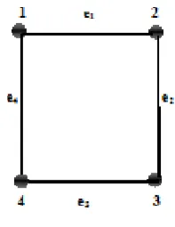
Definition 2.15: Series graph:

Let G = (V, E) be a graph with n vertices and m edges .The graph G is called a series graph if the induced weight (wind(e)) remains constant across all edges of the graph G and satisfying the equation w(vi) – w(vi+1) = w(ej)wind(e) (𝒊 ≠ 𝒋,𝒊=𝟏 𝒕𝒐 𝒏,𝒋=𝟏 𝒕𝒐 𝒎) where w(ej) is the actual weight (weight assigned to the edge ‘e’).

Let us demonstrate this concept with an example

Figure - 1: Series graph

Let w(1), w(2), w(3) , w(4) ,wind(e1) , wind(e2), wind(e3) and wind(e4) respectively represents the weights of the vertices and induced weight on the edges of the graph. From the above definition we represent the relation between the weights as follows

w(1) – w(2) = w(e1) wind(e1), w(2) – w(3) = w(e2) wind(e2), w(3) – w(4) = w(e3) wind(e3) and w(4) – w(1) = w(e4) wind(e4) .

Since in a series circuit the induced weight remains constant (i.e wind(e1) = wind(e2) = wind(e3) = wind(e4) = w(e) ) , thus we have w(1) – w(2) = w(e1) wind(e), w(2) – w(3) = w(e2) wind(e), w(3) – w(4) = w(e1) wind(e) and

w(4) – w(1) = w(e1) wind(e).

Definition 2.16: Parallel graph:

Let G = (V, E) be a garph with n vertices and m edges. The graph G is called a parallel graph if the ratio of the weights on the edges is equal to the ratio of the induced weight on the corresponding edges.

i.e 𝒘(𝒆𝒊)

𝒘(𝒆𝒊+𝟏)=

𝒘𝒊𝒏𝒅(𝒆𝒊+𝟏)

Let us explain this concept with an example as shown below

Figure - 2: Parallel graph

Let w(1), w(2), w(3), w(4), w(5), w(6), w(7), w(8), wind(e1), wind(e2), wind(e3) and wind(e4) respectively represents the weights of the vertices and induced weight on the edges of the graph. From the above definition we represent the relation between the weights as follows

w(1) – w(2) = w(e1) wind(e1), w(3) – w(4) = w(e2) wind(e2), w(5) – w(6) = w(e3) wind(e3) and w(7) – w(8) = w(e4) wind(e4). Since in a parallel graph the weights on the vertices remains constant (i.e w(1) – w(2) = w(3) – w(4) = w(5) – w(6) = w(7) – w(8) .

If w(1) – w(2) = w(3) – w(4) ⇒ w(e1) wind(e1) = w(e2) wind(e2) ⇒ 𝑤(𝑒1)

𝑤(𝑒2)=

𝑤𝑖𝑛𝑑(𝑒2)

𝑤𝑖𝑛𝑑(𝑒1).

Similarly w(3) – w(4) = w(5) – w(6) ⇒ w(e2) wind(e2) = w(e3) wind(e3) ⇒ 𝑤(𝑒2)

𝑤(𝑒3)=

𝑤𝑖𝑛𝑑(𝑒3)

𝑤𝑖𝑛𝑑(𝑒2)

and w(5) – w(6) = w(7) – w(8) ⇒ w(e3) wind(e3) = w(e4) wind(e4) ⇒ 𝑤(𝑒3)

𝑤(𝑒4)=

𝑤𝑖𝑛𝑑(𝑒4)

𝑤𝑖𝑛𝑑(𝑒3).

Definition 2.17: A linear graph:

An edge ‘e’ on which the labels ( w(e) = weight of the edge, wind(e) = induced weight on the edge) are constant is called an linear edge ‘e’. A graph with linear edges is called a linear graph.

Definition 2.18: Equivalent graphs:

Two graphs G and G/ are said to be equivalent if ‘l’ is the label on the edge of a graph G then the label on the corresponding edge in G/ is either l = l1 + l2 or l1l2 = l(l1 +l2).

Some important theorems and results in graph theory

Theorem 1: [6] A digraph is an Eulerian digraph if and only if G is connected and balanced.

Theorem 2: [6] A connected graph G is an Euler graph if and only if all the vertices of G are of even degree.

Theorem 3: [6] Kuratowski’s graphs K5 and K3,3 are non planar .

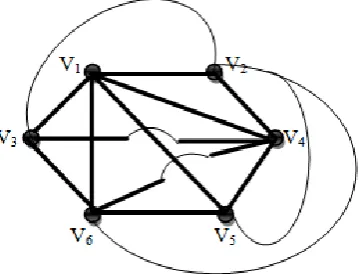
Remarks: In Kuratowski‘s non planar complete graph K5 atleast one edge intersect the other. We see that a non planar complete graph of six points alteast two edges intersect and continuing like this we conclude that in a non planar complete graph of n points atleast n−4 edges intersect. This is demonstrated in the following examples.

Let us consider a complete graph with six vertices.

From the figure we see that a complete graph with six vertices atlaest two edges cross over.

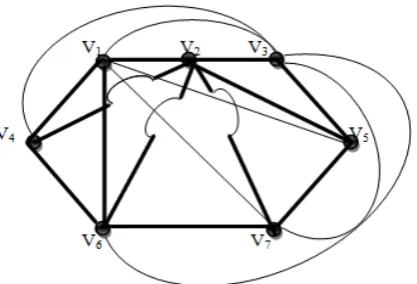
Let us consider another complete graph with seven vertices

Figure - 4: A non planar graph with seven vertices

From the figure we see that a complete graph with seven vertices atleast three edges cross over.

Definition 2.19: Electrical Network / Circuit: [8]

An electrical network/circuit is an interconnection of electrical components such as resistances, capacitances, inductance, etc connected to a voltage source. The electrical components of the circuit/network are mounted on circuit boards.

Definition 2.20: Edge and vertex in an electrical network/circuit:

Any electrical component in an electrical network/circuit is called an edge and its end points (or terminals) are called vertices.

Definition 2.21: Dummy vertex and Dummy Edge:

The terminals and interconnection between them in a PCB are called dummy vertices and dummy edges of the PCB (is a plastic board with terminals and interconnection between them).

Figure - 5: A Printed circuit Board

Definition 2.22: Dummy labeled PCB:

In a PCB [7] sometimes there is an indication on the interconnection between the terminals about the capacity of the electrical equipments to be used. Such a PCB is called a dummy labeled PCB.

Definition 2.23: A labeled PCB:

A PCB in which the interconnection between the terminals are equipped with a electrical component of the specified capacity is called a labeled PCA (Printed circuit assembly). A PCA is called a labeled PCB.

Figure – 7: A Labeled PCB (PCA)

Definition 2.24: Electrical walk/ path/trail/length:

A finite alternating sequence of terminals and electrical components is called an electrical walk If its vertices /edges are distinct then the walk is accordingly called a path/trail. The sum of the edges of the trail is defined as the length of the trail.

Definition 2.25: Electrical closed walk/Circuit/Cycle:

An electrical closed walk is a closed circuit / distinct electrical components /distinct terminals is called an electrical closed walk/circuit/cycle.

Definition 2.26: Connected/Disconnected network:

An electrical network in which there is atleast one path/no path between every pair of terminals is called a connected network, otherwise it is called disconnected.

Definition 2.27: Electrical Eulerian circuit/Hamiltonian cycle:

A circuit/cycle which contains all the electrical components/ traverses all the terminals of an electrical network is called an Electrical Eulerian circuit/ Electrical Hamiltonian cycle.

Definition 2.28: Electrical Eulerian graph/Hamiltonian graph:

An electrical network with an electrical Eulerian circuit/ Hamiltonian cycle is called an Electrical Eulerian graph/ Hamiltonian graph.

Definition 2.29: Series circuit: [8]

In series the components are connected along a single path, so that the same current flows through all of the components. A circuit composed solely of components connected in series is known as a series circuit [3]: Properties of series circuit

• The sum of the voltage drops is equal to the applied voltage.

• The total resistance of the circuit is equal to the sum of all series resistance. i.e if R1 and R2 areresistors connected in series then the total resistance R = R1 + R2

• The current through all the resistors of the circuit is same.

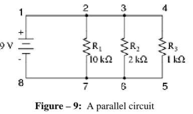
Definition 2.30 Parallel circuit: [8]

A parallel circuit has two or more paths for current to flow through the circuit. Such connections are also called multiple connections or shunt connections. In parallel circuits different branch loads operate independently of each other. Hence if any one load is disconnected or turned off the other branch loads continue to operate. Properties of parallel circuits

• The voltage across each branch is same.

• The current across each branch is given by V/R.

• Sum of the branch current is equal to the total current supplied by the battery.

• If R1 and R2 areresistors connected in parallel then the total resistance R = 𝑅1𝑅2

𝑅1+𝑅2

Figure – 9: A parallel circuit

Definition 2.31: Linear network: [2]

An electrical network is said to be linear if the circuit parameters (resistance, capacitance, inductance, frequency etc) are constant.

Definition 2.32: Port: [2]

A port is a two terminal connection in which the current into one terminal is identical to the current out of the other terminal.

Laws governing electrical network/circuit

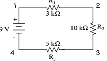
Definition 2.33: Ohm’s Law: [1]

If an electrical circuit is energized by an dc voltage there exists a definite relationship between current ‘I’ that flows through the resistance ‘R’ and the voltage ‘V’ applied across the resistance. i.e V = IR.

Ohm’s law gives the linear relationship between voltage drop across a circuit element and the current flowing through it. Therefore the resistor R is viewed as a constant independent of the voltage and current.

2.31: Kirchhoff’s laws: [1]

Definition 2.33.a) Kirchhoff’s Voltage Law:

Kirchhoff’s voltage law states that “the algebraic sum of all the voltages in a closed loop is equal to zero”.

Definition2.33.b): Kirchhoff’s current law:

Kirchhoff’s current law states that “the algebraic sum of the currents at a node or junction is equal to zero”. It can also be states as the sum of currents entering a node is equal to sum of currents coming out of that node. The circuit under this condition is called a balanced circuit.

Theorems and results in electrical network theory

Theorem 4: Thevenin’s theorem [8]

The theorem states that a linear two terminal circuit can be replaced by an equivalent circuit consisting of a voltage VTH in series with a resistor RTH where VTH is the open circuit voltage and RTH is the input or equivalent resistance at the terminals when the independent source is turned off.

Theorem 5: Maximum power transfer theorem [8]

SECTION-3

This section is purely devoted to representing an electrical network by a graph and conversely.

An electrical network/circuit and its graph: [4]

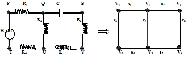
The graph G = (V, E) represents a circuit with the vertex set V representing the terminals and the edge set e representing the electrical components. For example, here is a circuit and its graph.

Figure – 10: An electrical circuit and its graph

The set V of vertices is = {V1, V2, V3, V4, V5, V6} and the set E of edges is = {e1, e2, e3, e4, e5, e6, e7}. Figure 7 shows how an electrical circuit can be represented by its corresponding graph.

Now let us see how we can uniquely represent an electrical circuit from a given labeled graph

Let us demonstrate to show how a labeled graph gives rise to more than one circuit.

This non uniqueness is caused by the fact that we are free to put any component on these edges, since they are not specifically labeled .By specific labeling of an edge we can almost build a unique circuit.

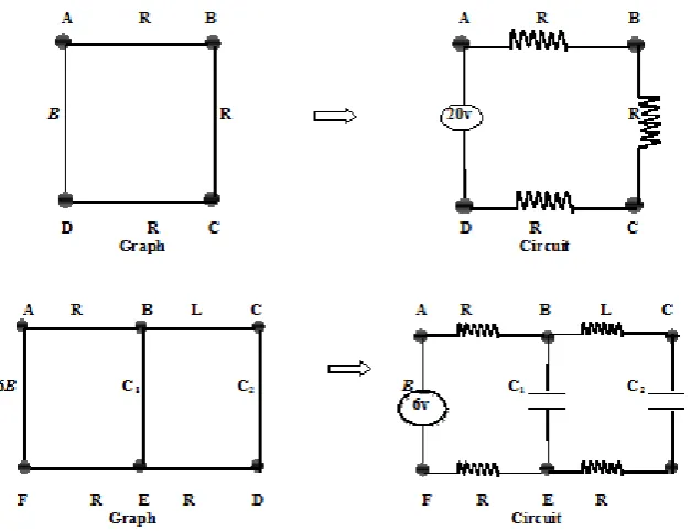
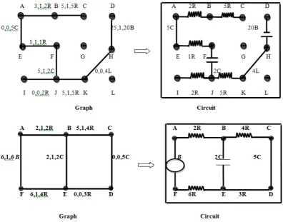
To achieve uniqueness we label the graph and demonstrate this with the following examples.

Figure – 12: Labeled graphs and their corresponding electrical circuits

From the above examples we see that labels on the edges of the graph specifies the electrical component to be equipped between the terminals in the corresponding circuit. We say that the corresponding circuit is almost unique, since the labels do not indicate the “units” of the component. Mere labeled graphs does not give unique graph.

To achieve better uniqueness the edges are multi-labeled indicating an electrical component along with its value as demonstrated in what follows

The edge AB indicates a resistor with 3 units, edge BC indicates inductance with 2.5 units edge CD represents resistor of 1 unit and edge AD representing battery of 20 units. Similar explanation holds good for other graphs.

Now let us see how we can represent an electrical network/circuit as its corresponding labeled graph (or multi – labeled Graph).

Figure – 14: An electrical circuit and its multi-labeled graph

The above example demonstrate the mutual translations of an electrical network and conversely.

Now let us now demonstrate how we can represent a graph for a given PCB and conversely.

A PCB is a plastic board equipped with electrical component between the terminals. The graph representing a PCB (Figure 5) is purely geometrical as shown below.

Figure - 15: Graph of a PCB

The edges of the PCB are called dummy edges and the end points edges are extended to terminals are called dummy vertices.

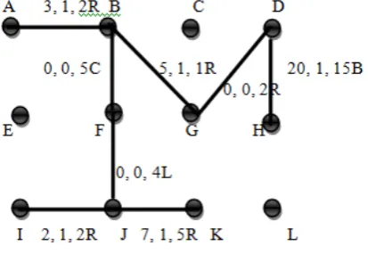
In a PCB the interconnection between the terminals are equipped with a electrical component of the specified capacity. Such a PCB is called a printed circuit assembly (PCA). The graph corresponding to a PCA (Figure 7) is called an edge labeled graph. Each edge of the graph has two labels one indicating capacity of the interconnection and the other indicating the capacity of the component. Sometimes the edge labeled graphs has three labels. The first label indicating the capacity of the interconnection, the second indicating the presence of the electrical component (either 0 or 1) and the third indicating the capacity of the component as shown in the figure

Figure – 16: Graph of a PCA (Labeled PCB)

Figure – 17: Graph of a PCA and its corresponding PCA

From the above examples we see that by using the definition of a dummy vertex, dummy edge and labeled edge of a graph representing a PCB, we can uniquely represent the graph of the electrical network and conversely.

An electrical version of Kuratowski’s theorem is a complete network is short circuited with ten electrical component as shown in the figure

Let us drawn an electrical network for Kuratowski’s complete graph with five vertices

Figure – 18: Graph of a PCA and its corresponding PCA

SESSION-4:

In this session we see that how some theorems in graph theory finds its natural application to electrical networks/circuits and conversely. Here we verify the theorem1 by taking an example and represent its corresponding electrical circuit.

Figure – 19: An Eulerian digraph

From the figure we see that the given digraph is an Eulerian digraph which is connected and balanced (i.e d+(v) = d-(v)) Conversely the given digraph which is connected and balanced is an Eulerian digraph. Thus verifying the theorem.

We first formulate theorem 1 in terms of electrical networks and also translate the Eulerian digraph in figure 16 to electrical networks/circuits and see how the theorem1 holds. In this connection we observe that

• When an electrical network is energized with an voltage supply there is flow of current across each electrical component in the network, thus resulting in a closed and connected network.

• Flow along an edge refers to flow of current between two terminals (potential difference between the two terminals).

• At each terminal we see that the sum of currents entering a node is equal to sum of current leaving that node.

The electrical version of theorem 1 is

Theorem 1.1: An electrical network/circuit is an electrical Eulerian network if and only if the network is connected.

Note: The condition in the theorem that the graph is balanced is automatically satisfied by Kirchhoff current law in a PCB.

We now demonstrate the verification of the theorem 1 by constructing the circuit for the given Eulerian digraph (figure 19).

Figure – 20: The electrical circuit for the Eulerian digraph (figure 16)

From the figure 17 we see that the electrical network/circuit is connected and balanced [KCL].Conversely we see that a network which is connected and balanced is an electrical Eulerian network .Thus verifying the theorem1.1

Figure – 21: A closed electrical network/circuit

Note: When an electrical network is translated to its corresponding graph the theorem 1 holds good only when the graph has vertices of even degree (theorem 2).

The corresponding digraph is given in the following figure

Figure – 22: The digraph of the electrical network (figure 21)

Observations: We see that the given digraph is Eulerian diagraph which is connected. The number of indegree and outdegree for each vertex in the digraph is given from the following table

Vertex Indegree Outdegree

1 1 1

2 2 2

3 1 1

4 2 2

5 2 2

6 1 1

From the table we see that at each vertex indegree is equal to outdegree. Hence the given digraph is balanced. Thus we see that given a digraph it is Eulerian if and only if it connected and balanced.

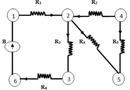
Now let us demonstrate how theorem 4 of electrical network can be translated in terms of graphs.

Figure – 23: An electrical network

Following are the steps involved solve the given electrical network to an equivalent series network with Thevenin’ voltage VTH and equivalent resistance RTH to find the voltage and current flow across the resistor of 12Ω.

Step-1: Disconnect the 12Ω resistor from the terminal A and B, then the network is as follows.

Figure – 24: An electrical network with Thevenin’s voltage VTH

Step-2: With the load terminals A and B open, the open circuit voltage VOC is equal to the voltage drop across the 6Ω resistor because point A is at the same potential as at point C. This voltage drop is the Thevenin’s voltage VTH across the terminals A and B.

Calculation of VTH

VTH = VCD = I x 6 where VCD is the voltage drop across the terminals Cand D and I is the current in the circuit. I = 36(3 +6) = 4 A

Therefore VTH = 4 x 6 = 24V

Step-3: Replace the battery with a short circuit resulting in no internal resistance in the circuit and the equivalent resistance RTH of the circuit is calculated.

Calculation of RTH

We have resistor R1 in series with the resistor R3 and in parallel with the resistor R2. Therefore the equivalent resistance of the circuit is given by RTH = 4 + 6₆₊₃×3 = 6Ω.

Step-4: Having found the Thevenin’s voltage VTH and the equivalent resistance RTH, the circuit is connect back in series with the source as shown.

Figure – 26: An equivalent circuit for the electrical network (Figure 23)

Let us interpret the theorem 4 in terms of graphs and see how the theorem holds.

The graph theoretical version of theorem 4 is

Theorem 4.1: Any linear graph G can be replace by its equivalent graph G/ having lesser number of edges.

We now demonstrate the verification of the theorem 4 by constructing the graph for the electrical network (figure 23).

Figure – 27: Graph corresponding to the electrical network in figure 23

Now by applying the steps involved in Thevenin’d theorem we get the equivalent graph for which we can calculate the induced current across any particular edge.

Figure – 28: Equivalent graph for the graph in figure 26

Note: The converse is not unique.

CONCLUSION

REFERENCES

1. Alexander , C ,K., Sadiku , M , N.,: Fundamental of electric circuit , New York , MaGraw – Hill, 2004 2. Carson, A, B., Circuits: Engineering concepts and analysis of linear electric circuits, Standford, C.T .Brooks

cole, 2000.

3. Douglas Brent West, Introduction to graph theory, Prentice –Hall of India, private limited, 2014. 4. Foulds, L, R.,: Graph theory application, Springer science and Business media, 1995.

5. Frank Harary, Graph theory, Addison – Wesley, MA, 1969.

6. Narsingh Deo, Graph theory with application to Engineering and Computer science, Prentice –Hall of India, private limited, 1990.

7. Sampathkumar, E.,Sriraj,M,A , Vertex labeled/colored graphs, matrices and signed graph: Information and System Sciences, Vol. 38(2013),No-1-4,pages 113-120.

8. Theraja, B,L,: Basic electronics, First edition, S.Chand & company Ltd, 2012.

Source of support: Nil, Conflict of interest: None Declared.