ISSN 2307-7743 http://scienceasia.asia
APPLICATION OF CONE-GRID SCHEME FOR SOLVING BURGERS EQUATION
MAHMOUD A.E. ABDELRAHMAN
Abstract. The cone-grid scheme for the Burgers equation is introduced, which gives exact
unique solutions. The Riemann solution for the Burgers equation is the building blocks for this scheme. To validate this method and assess its accuracy, front tracking scheme is also applied to the same model. These two schemes are compared by interesting numerical examples, where the explicit solutions are known.
1. Introduction
In this paper we consider the Burgers equation, which given in the following form :
(1.1) ut+
u2
2
x
= 0,
which we can write in the form
(1.2) ut+uux = 0.
The numerical solution of Burgers equation is so importance due to the equations appli-cation in the approximate theory of flow through a shock wave travelling in a viscous fluid and in the Burgers model of turbulence.
The front tracking and the cone-grid schemes could serve as a common numerical technique to solve several scientific and engineering problems due to avoiding the specific eigenstruc-ture of the problem [1]. In fact the Riemann solution for the Burgers equation is the basic ingredients for these schemes. These schemes have also high order accuracy in smooth re-gions of the simulated flow and resolve sharp discontinuous profiles in the shock rere-gions.
In [1] we presented a new schemes for the first time, namely the cone-grid scheme. Here we will show that the Burgers equation equations give an surprisingly explicit algebraic solu-tion. The cone-grid scheme also gives a powerful shock resolusolu-tion. Hence the cone-grid and front tracking schemes enable us to give an instructive comparison with each other as well as with well known exact solutions, for example the exact Riemann solutions. Two numerical examples studies are carried out.
Key words and phrases. Cone-grid scheme, Burgers Equation, conservation laws, shock waves, entropy conditions, rarefaction waves.
c
2016 Science Asia
In this paper, the cone-grid scheme is implemented for solving Burgers equation in one space dimension. For validation and comparison, the numerical results of front tracking schemes is also presented [3].
The paper is organized as follows: Section 2 gives a brief description of the Burgers equation. The one-dimensional cone-grid scheme is briefly presented in Section 3. In Section 4, one-dimensional numerical test problems are given. Finally, in Section 5 the conclusions are summarized.
2. The Riemann Problem
A Riemann problem for the Burgers equation, consists of a conservation law,
(2.1) ut+
u2 2
x
= 0,
together with a piecewise constant data having a single discontinuity,
(2.2) u(t, x) =
(
u−, x≤0,
u+, x >0.
The form of the solution depends on the relation between u− and u+.
• Case1. If u− > u+, in this case there is a unique weak solution,
(2.3) u(x, t) =
(
u− xt < s
u+ xt > s
,
where
(2.4) s= u−+u+
2
is the shock speed, the speed at which the discontinuity travels.
• Case 2. If u− < u+, in this case there are infinitely many weak solutions. One of these is again (2.3) and (2.4) in which the discontinuity propagates with speed s. Another weak solution is the rarefaction wave
(2.5) u(x, t) =
u−, xt < u−
x
t, u−< x t < u+
ur, xt > u+
,
For more details about the Burgers equation we refer to the textbooks [2], [4] and [5].
3. Cone-grid scheme
In this section, the cone-grid scheme is derived [1]. The one-dimensional Burgers equation for numerical purposes may be written down in the dimensionless “vector form ”,
u′ − u′ + ˜ Ri e m an n s o lu ti o n light cone u− u+ Ω xj,k−1
tj−1 tj tj+1
xj,k
xj,k+1x
t
u
Figure 1. Balance
re-gions [1] .
slope-Λ ≤-1
slope Λ≥ 1 α′ α β′ β 0 T x
2(M+N) grid cells of length ∆x output domain t Figure 2. Computational domain [1].
In this section we review the cone-grid scheme, which is discretized in time and space. This scheme is based on the integral conservation laws in terms of curve integrals acclimatized to the choice of the numerical time and space grids. Moreover we will prove that this scheme admits a unique weak solution for the Burgers equation.
This scheme is very interesting and can be obtained easily from the conservation laws on a cone-grid. We describe a fixed time step ∆t >0 and calculate the spatial mesh size ∆xin terms of the natural Courant-Friedrichs-Lewy (CFL) condition, which is satisfied.
We consider the Riemann solution of the Burgers equation inside the cone depicted in the Figure 1 in order to derive the cone-grid scheme. For the construction of the cone-grid scheme, we use the conservation laws with respect to the computational domain depicted in Figure 1, namely
(3.2)
I
∂Ω
u(t, x)dx−F(u(t, x))dt = 0.
3.1. The computational domain. Before applying the scheme, it is necessary to discretize the computational domain. The computational domain is the trapezium in Figure 2. Recall
λ:= max
a≤u≤b|f
0 (u)| .
Given are α and β ∈ R, withα < β, T >0 and M ∈N, which give the number of grid cells for the half of the space interval [α, β], i.e.
(a) The spatial mesh size is
(3.3) ∆x:= β−α
xj,k Ω + j,k
Ω−j,k
ν1
ν2
ν3 ν4
tj−1 tj tj+1
∆t u+
u−
u′
+
u′
− x
t
Figure 3. Balance cell[1].
(b) The number
(3.4) N :=
T
∆x
=
2λT M β−α
is the smallest integer such thatλ . T ≤N·∆x, where the ceiling functiondye is the smallest integer larger than or equal y.
(c) Put ∆t:= 2TN. ThenT = 2N∆t. Hence, using 1 and 2 we have
(3.5) λ <Λ := ∆x
2∆t =
∆x·N
T ,
where the CFL-condition is satisfied. N gives the grid cells number’s for the half of the time interval [0, T] and ∆t the time step size i.e. the interval [0, T] divided into 2N sub intervals of length ∆t.
(d) We have the time discretization tj =j ·∆t for j ∈ {0, ...,2N}.
(e) We define the quantities
(3.6) α0 =α−T ·Λ, β0 =β+T ·Λ,
which give the bounds of the trapezium domain on the x-axis to avoid the artificial numerical boundary effects, see Figure 2. The spatial intervals [α0, α], [β, β0] split intoN sub intervals of length ∆x.
(f) At time tj−1 we define the grid points
xj,k =α0+ (j−1) Λ·∆t+ (k−1) ∆t, j = 1, ...,2N + 1, k= 1, ...,2(M +N)−j+ 2.
We note that the quantitiesxj,k determine all points of each balance cell in Figure
1. Especially we can easily check that x1,1 =α0 and x1,2(M+N)+1 =β0 at initial time
t0 = 0 as well asx2N+1,1 = α and x2N+1,2M+1 =β at final time t2N =T, which give
3.2. The construction of the solution. In this section we consider a restriction to spatial grid points that gives the left corner points of each balance cell in Figure 1 as well as in Figure 3. In these balance cells we will solve the local Riemann problems. For the left corner-point
ν1 given by ν1 = (tj−1, xj,k) in Figure 3 we solve the local Riemann problem
ut+uux = 0,
u(tj−1, x) =
u− if x≤xj,k
u+ if x > xj,k
for t > tj−1 and assume that the numerical solution inside the parallelogram is given by
u(t, x).
Especially the constant value ofu(t, x) along the cord connectingν1withν3will be denoted by ˜
u. Consider the triangular balance regions Ω+j,k and Ω−j,k , spanned by the points ν1, ν3, ν4 and ν1, ν2, ν3, respectively, see Figure 3 . On each cord ν2ν3 and ν3ν4 we replace the numerical solution by the unknown constant values u0− and u0+, which require that
(3.7)
Z
∂Ω∓j,k
udx−F(u) dt= 0.
For the balance region ∂Ω+j,k, using 3.5 we obtain:
(3.8) u0+−u+− 1 Λ
h
2 F(˜u)−F(u0+)−F(u+)
i = 0,
i.e. an implicit equation for u0+.
For the balance region∂Ω−j,k we obtain in the same way the following implicit equation for
u0−:
(3.9) u0−−u−+ 1 Λ
h
2 F(˜u)−F(u0−)−F(u−) i
= 0.
The new statesu0∓turn out to be uniquely calculated by using 3.8, 3.9 and the CFL-condition Λ≥1.
Note that for fixed values of α,β and T the quantity Λ in (3.5) depends on M, such that we can also rewrite it in the form Λ = ΛM. Then we conclude from (3.3), (3.4) that
lim
M→∞ΛM = 1. Complete derivation of the scheme introduced in [1].
Lemma 3.1. Let be u−≤u+. Then equation (3.8) has a unique solution u
0
+ ∈[˜u, u+], and (3.9) has a unique solution u0−∈[u−,u˜].
Proof. For u− = u+ it follows u− = u+ = ˜u = u
0
+ = u
0
−, hence assume u− < u+. By the formal replacements F 7→ −F,u− 7→u+ and u
0 − 7→u
0
+ equation (3.9) reduces to (3.8) . It is thus sufficient to prove the existence and uniqueness foru0+:Assume first thatu0+ < u00+
are two different solutions. Then
u00+−u0+ =−2∆t ∆x(F(u
00
+)−F(u
0
+)) >0,
and
u00+−u0+ = −2∆t ∆x(F(u
00
+)−F(u
0
+))
= 2∆t ∆x
F(u00+)−F(u0+)
u00+−u0+
(u00+−u0+)
≤ 2∆t ∆x λ (u
00
+−u
0
+)
< (u00+−u0+)
from the CFL-condition, which is a contradiction. It remains to show the existence for u0+ : It follows from the convex-hull construction of ˜u that
(3.10) F(˜u) = min
u−<u<u+
F(u).
DefineB : [˜u, u+]7→Rby
B(u) = u−u+−2 ∆t
∆x(F(˜u)−F(u)−F(u+)).
Then from the CFL-condition:
B(˜u) = u˜−u++ 2 ∆t
∆x(F(u+)−F(˜u))
≤ u˜−u++ 2 λ ∆t
∆x(u+−u˜)
= (˜u−u+).(1−2 λ ∆t
∆x)
| {z }
>0
≤0
(3.11)
and from (3.10) :
(3.12) B(u+) = 4
∆t
∆x(F(u+)−F(˜u))≥0.
Then from (3.11), (3.12) and the mean value theorem we obtainB(u0+) = 0 for an appropriate
−1
1
t= 1
0
−1 1
x
t
−1
1
t= 1
0
x
t
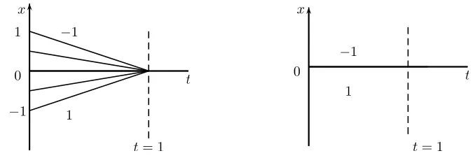
Figure 5. Two different initial data give the same solution at t= 1 .
4. Numerical examples
In this section we introduce numerical examples for the solution of Burgers equation. We use the exact Riemann solution, cone-grid and front tracking schemes for the comparison. We will show that how the cone-grid is powerful scheme to solve Burgers equation.
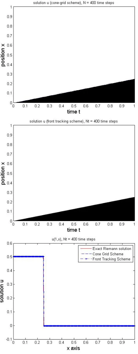
Example 4.1. Single shock solution of the Burgers equation.
In this example we test our cone-grid and front tracking schemes for a single shock problem. We supplied initial data to the program for which we know that a single shock solution results from the Rankine-Hugoniot jump conditions. We select the initial data and the space-time range such that the shock exactly reaches the left lower corner at the time axis. Figure (4)1,2 represent the plots of the solution in the time range 0 ≤ t ≤ 1 and in the space range 0≤ x≤1. The figures shows that cone-grid and front tracking schemes captures this shock in exactly the same way as predicted by the RankineHugoniot jump conditions. The Figure 4 3 presents the solution at the fixed time t = 1 for the same initial data. The Riemannian initial data is chosen as
u= 0.25∗(1−sign(x))
where 400 mesh points are considered here. In this example we found that our cone-grid and front tracking schemes gives a sharp shock resolution. This is a good test for the front tracking scheme, and its success indicates that the entropy inequality is satisfied.
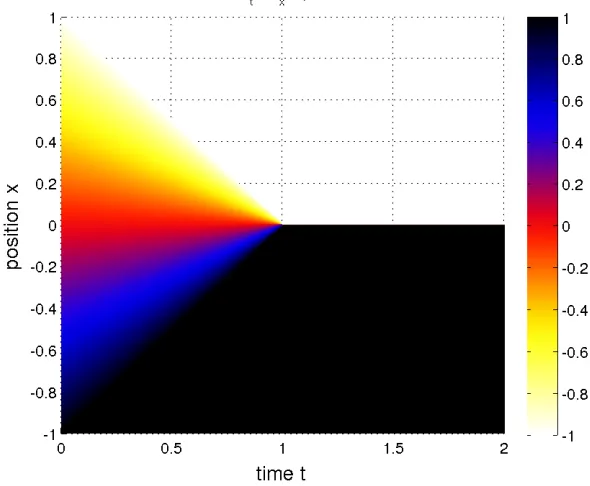
Example 4.2. An example of the irreversibility for the Burgers equation.
Figure 6. Burgers solution for 0< t <2.
We define u1(t, x) to be a solution of the equation (2.1), which present the compression wave, for 0 ≤t < 1 we set
(4.1) u1(t, x) =
1, x≤t−1,
x
t−1, t−1< x≤1−t,
−1, x >1−t.
We define u2(t, x) to be a solution of the equation (2.1), which present the single shock, we set
(4.2) u2(t, x) =
(
1, x≤0,
−1, x >0.
Theu1,2 are depicted in Figure (5). It is easy to check that they are all solutions, moreover, each of u1,2 satisfies the entropy condition.
Thus they are all correct solutions. The point that we wish to emphasize here is that all of these solutions coincide at t= 1:
(4.3) u(1, x) =
(
1, x≤0,
−1, x >0.
We emphasize again that all of these solutions are the right ones, in that they belong to the class of solutions, which are uniquely determined by their initial values. But this uniqueness is only in the direction of increasing t. Two solutions in this class which agree at t= 1 must be equal for all t > 1, but need not be equal for t < 1. It is in this strong sense that solutions of conservation laws do not have backward uniqueness.
The numerical simulation in Figure 6 serve for illustration the non-backward uniqueness using cone-grid scheme.
5. Conclusions
In this paper we described the cone-grid scheme for the Burgers equation numerically. Moreover, we have shown that this scheme admits a unique solution. The cone-grid scheme also gives a powerful shock resolution.
We implemented the cone-grid and front tracking schemes numerically. Hence, we introduce numerical test examples for the solution of the Burgers equation. For the interesting com-parison we use the exact Riemann solutions for the cone-grid scheme as well as for the front tracking scheme. Finally, the numerical examples are given.
References
[1] M.A.E. Abdelrahman and M. Kunik, A new Front Tracking Scheme for the Ultra-Relativistic Euler Equations, J. Comput. Phys. 275 (2014), 213-235.
[2] R. Courant and K. O. Friedrichs,Supersonic flow and shock waves, Springer, New York, 1999.
[3] M. Kunik, Lecture Note on Numerics for Hyperbolic Conservation Laws, Otto-von-Guericke University Magdeburg, (2012).
[4] R.J. LeVeque. Numerical Methods for Conservation Laws, Birkh¨auser Verlag Basel, Switzerland, 1992.
[5] J. Smoller. Shock Waves and Reaction-Diffusion Equations, Springer-Verlag New York Heidelberg Berlin, 1st edition, 1994.
![Figure 3. Balance cell[1].](https://thumb-us.123doks.com/thumbv2/123dok_us/7820737.2087551/4.612.215.399.71.240/figure-balance-cell.webp)