Spatial Analysis of the Effect of Noise on the Prices and Value of Residential Real Estates

Rados³aw Cellmer*

Spatial Analysis of the Effect of Noise

on the Prices and Value

of Residential Real Estates

1. Introduction

A steadily growing number of areas exposed to noise and the resulting detri-mental effects on the usable value and the prices of real estate may pose a signifi-cant problem in the process of managing real estate in urban areas.

Pursuant to the provisions of the EU Environmental Noise Directive 2002/49/EC, the key document for the assessment and management of environ-mental noise, and the Polish Environenviron-mental Protection Law, Poland is under obli-gation to perform acoustic audits and develop action plans for areas where noise levels exceed the relevant limit values.

The provisions of the Environmental Protection Law place county administra-tors under the obligation to develop and update noise maps every five years. The maps support the assessment of exposure to noise, they identify the main sources of noise and areas where the relevant limit values are exceeded. The information presented in noise maps serves merely as guidance on the degree of noise emis-sions in a given area, and it indirectly points to the resulting decrease in real estate prices. Information on the harmful effects of excessive noise on local property markets, in particular transaction prices and real estate prices, would significantly contribute to the development of effective action plans to enhance the usable value and prices of urban property.

The aim of this study was to present the methodology and the results of spa-tial analyses investigating the impact of noise on the average prices of residenspa-tial real estate in the city of Olsztyn in north-eastern Poland.

13

* University of Warmia and Mazury, Department of Real Estate Management and Regional Devel-opment, Olsztyn, Poland

2. Literature Review

Noise generated by street traffic is one of the most detrimental factors that af-fect the usable value of urban space and, consequently, real estate prices. The im-pact of noise on market prices may be assessed by analyses of primary sources, such as market surveys, as well as statistical models investigating cause and effect relationships, mostly regression models [25]. The advantages of market surveys over econometric models have been discussed by Smith and Mansield [23]. None-theless, market surveys often deliver subjective information regarding noise an-noyance, and the respondents are frequently unable to relate the above factor to the economic value of property [22]. Unlike surveys, statistic models rely on trans-action prices which reflect the actual decisions made by market participants and not only their readiness to make purchase decisions. It should be noted, however, that analysis results are also largely determined by the choice of variables and the functional form of the model. The first regression models accounting for the effect of road traffic noise on property prices have been developed many years ago by Nelson [20], Hughes and Sirmans [13], Bateman et al. [5], Wilhelmsson [29] and Huang and Palmquist [12]. As rightly noted by Bateman et al. [5], regression mod-els illustrating the effect of noise on prices aim to explain price variability with the use of selected property characteristics, including annoyance caused by exposure to road traffic. Bateman points out that prices are determined by the specific at-tributes of the local market, and, above all, they reflect the relationship between demand and supply which are very difficult to quantify. The above author pres-ents detailed results of modeling the effects of noise on property prices, including the demand for peace and quiet, for different market segments.

The noise depreciation sensitivity index (NSDI) is a robust measure of noise effects on real estate prices. NSDI determines the percentage depreciation in prop-erty prices per 1 dB increase in noise levels. According to Nelson [20] and Bate-man et al. [5], NSDI ranges from 0.4% to 0.5% for apartments on average. Similar analyses were carried out on the land market to show NSDI values as high as 1.3% [15]. NSDI values were also discussed by Blanco and Flindell [6] in a review of studies performed in the US, Canada and selected European cities. The use of spatial autoregressive models to determine NSDI values on the housing market was also discussed by Theebe [25] on the example of Amsterdam. Theebe argues that noise intensity and property prices are not always bound by a linear correla-tion. He supports his claim by stating that the sound intensity level expressed in decibels is a logarithmic, and not a linear, measure of noise intensity.

Other price-forming factors also significantly contribute to the effects of envi-ronmental noise. Real estate may vary substantially with regard to its legal and physical attributes. According to the regressive modeling approach, real estate

prices reflect variations such as size, age, technical condition and standard, which, when combined with other environmental factors, support the development of a correct model [6]. In a study modeling the effect of noise on property prices, Brandt and Maening [7] analyzed 20 attributes related to the real estate and its lo-cation, and his approach significantly improved the fit of the model. In Brandt’s study of the city of Hamburg, NSDI was determined at 0.23% at the significance level of 0.01.

In the above models, the noise effect on prices is generally regarded to be a stationary phenomenon which does not change in space. The above statement leads to the assumption that the two factors are bound by the same correlation at every point of the analyzed area. An alternative hypothesis, postulating that those dependencies vary in space, can also be proposed.

The principles for the spatial modeling of price-forming factors have been dis-cussed by Dubin [10] and Pace et al. [21]. The above authors examined the residu-als from a regression analysis to search for variables that have not been accounted for in the model and whose value is determined by location. Spatial correlations between noise intensity and prices were also investigated by Anderson et al. [2] who relied mostly on traditional regression models, but also noted that modeling errors are regularly distributed in space.

Spatial analyses can significantly enhance model significance, and they can accurately reflect the dependencies on the real estate market. To date, few authors have performed spatial analyses with the involvement of geographically weighted regression and geostatistical methods. For this reason, this study emphasizes the use of the above methods as tools that support an evaluation of spatial variation in noise effects on real estate prices.

3. Materials and Methods

The impact of environmental noise on the usable value and prices of residen-tial real estate was assessed with the involvement of both statistical and geostatistical methods. In the first stage of the study, a map of unit prices of apart-ments was developed by kriging interpolation. The above approach supported a comparison of the spatial distribution of prices and noise levels in the examined locations. ANOVA tests were performed to evaluate the impact of noise on real es-tate prices. To determine the spatial correlations between prices and noise inten-sity, a geographically weighted regression model (GWR) was built, and the spatial distribution of the strength and significance of the analyzed relationships was identified. Cokriging interpolation was used to generate a price distribution map where noise intensity was input as an additional variable.

The use of geostatistical methods in spatial analyses of the real estate market has been discussed by Anselin [3], Haining [11] and Leuanghton et al. [19]. The venture point for investigating spatial correlations on the property market can be the assumption that the interactions between the studied objects in space are char-acterized by spatial auto-correlation. Spatial auto-correlation is defined as the de-gree of correlation between a variable in a given location and the value of that variable in a different location. The problem of spatial auto-correlation on the real estate market has been discussed by Basu and Thibodeau [4], Ismail et al. [14], who analyzed the spatial distribution of residuals from a regression analysis by calculating semivariograms. Tu et al. [26] relied on the spatial auto-correlation phenomenon to suggest guidelines for the determination of property boundaries based mostly on spatial factors. The above authors also demonstrated that the spa-tial segmentation of the housing market can be performed with the use of the same method.

Kriging is a geostatistical method that provides the best, unbiased linear mators of a regionalized variable. Sample data (measuring points) inside the esti-mation area (sample search area) is assigned respective weight, referred to as kriging weight factors, in such a way as to minimize the mean squared error of es-timation (kriging variance). This method assigns greater weight to points situated closer to the observer, but weights are determined using a variogram or a semivariogram calculated from a classical semivariance estimator [4, 24]:

$( ) ( ( ) ( )) g h ni z si h z si n = + -=

å

wherez(si+ h) andz(si) are the values of the analyzed attribute at points separated by distanceh, and nis the number of the pairs of points separated by distance h. The semivariogram function, developed by mapping semivariance values depend-ent on distanceh in the chart, describes the structure of variability in the studied population. The weighted mean is determined using the below estimator:

$ _{( )} Zv w Z xi i i N = =

å

The weights determined by the semivariogram are assigned to produce esti-mators that are unbiased and characterized by minimal variance, referred to as kriging variance.

The most popular kriging estimators include ordinary kriging, which is used when the means are unknown, and simple kriging, which is applied in non--stationary models with a known mean for the entire population or for computing

local estimates of the mean. According to many experts [9, 24, 28, 31], kriging is the best method for interpolating non-heterogeneous natural phenomena because kriging algorithms contain procedures ensuring the minimization and random distribution of errors (the estimator is unbiased, which implies that negative and positive errors are balanced out). Kriging accounts for general data trends, and it is a useful method when data is not uniformly distributed. Kriging interpolation supports the estimation of the searched value at any point of the analyzed area. With the use of the above procedure, unit value can be estimated separately for each point, where points0, at which value is appraised, may be the geometric

cen-ter of any building containing the apartments in the studied area.

Co-kriging is a natural extension of the kriging technique when multi--dimensional data is available. The main variable is estimated in a given location based on auxiliary data and variables in the neighborhood. When prices and noise levels are highly correlated, their values can be used in conjunction to estimate ev-ery variable in succession. The ordinary co-kriging estimator represents the linear combination of weightswai with variables situated in the neighborhood of the

esti-mated pointx0[27]: Zi x w Z x i ni i N 0 0 1 1 * _{( )= ( )} = =

å

å

Co-kriging is generally applied when sufficient quantities of data relating to the main variable are not available, but there are vast quantities of reliable data on the spatial distribution of the additional variable which is significantly correlated with the main variable. The researchers have concluded that noise intensity can be an additional variable.

The relationship between prices and noise levels can be illustrated with the use of a classical regression model. In general, regression models fail to directly ac-count for potential interactions (spatial auto-correlation) between the intensity of a given phenomenon in space, and they assume that the price shaping process in geographical space is stable [17]. In this case, the significance of parameters in clas-sical regression models is not affected by the spatial structure of the studied phe-nomenon, which could lead to the misinterpretation of results [8], in particular on the assumption that real estate markets are characterized by spatial heterogeneity.

Various methods of accounting for the spatial structure of the studied phe-nomenon in regression models have been discussed in literature [3, 11]. One of the reviewed methods proposes to assign weights to observations which, owing to their location in space, could have a theoretically greater impact on the analyzed phenomenon than other observations. The above can be expressed with the use of geographically weighted regression.

Geographically weighted regression (GWR) is used on the assumption that the modeled parameters can be estimated separately at every point in space for which the values of the dependent variable and the independent variable are known. The interactions between the studied objects in space are often characterized by the ob-servation that elements found close to one another are more similar than objects that are far apart. The above principle can be used to estimate the modeled param-eters in a given location on the assumption that the observations made at points closer to the studied object will have greater weight than the more distant observa-tions [8]. A standard GWR model equation will take on the following form:

yi =b0( ,x yi i)+b1( ,x yi i)× +xi ei, (4)

or, for many independent variables:

yi =b0( ,x yi i)+b1( ,x yi i)×x1i +b2( ,x yi i)×x2i+ +... bm( ,xi y xi) mi + ei,

fori= 1, 2, ...,n (5)

The value of the modeled parameters is determined by location which, in this case, is expressed by coordinates (xi, yi). The parameters of the GWR model are es-timated similarly to classical models, but the weights of observations determined by location are taken into account:

$_{( , ) ( )} ( ) ( ) bx yi i X W X X W Y T i T i = -1 ₍₆₎

whereW(i)is the matrix of weights that are a function of the distance between the

location described by coordinates (xi, yi) and the location of every observation point. The above matrix takes on a diagonal form, and its elements can be ex-pressed in various ways, mostly [17]:

w d h ij ij = -æ è çç ö_ø÷÷ é ë ê ê ù û ú ú 1 2 2 (7)

where dij is the distance between locations i and j, and h is the bandwidth. The above parameter indicates the spatial range that generates observations for the cal-culations, indicating thatwij= 0 fordij> h.

The GWR model produces a series of fields mapped by the estimated parame-ters. The differences in the value of those parameters in space suggest that de-pendent variables’ effect on the indede-pendent variable and, consequently, the spa-tial heterogeneity of the examined phenomenon are characterized by local vari-ance [8]. Since parameter estimation takes place at selected points in space, local variance at any given point may be determined by spatial interpolation, and the result may be presented in map form (such as an isarithmic map).

4. General Characteristics of Source Data

Analyses were carried out in the city of Olsztyn in north-eastern Poland. Olsztyn has an estimated population of 180,000, and it covers the area of more than 88 km2. Environmental factors play an important role in the investigated re-gion owing to an abundance of natural features, including lakes and forests within Olsztyn’s administrative boundaries. The main source of noise is road traffic, and it is intensified in the afternoon in the city’s busiest streets. The annoyance effects of railway and industrial noise are less profoundly experienced.

The main source of information on noise intensity is a noise map which de-scribes the present and forecast acoustic environment of the area, including a graphic presentation in the form of several data layers on a base map [16]. Noise maps are developed to assess the acoustic climate of the examined region and to develop noise abatement programs [18].The information on noise intensity levels for the studied area was obtained from a noise map of Olsztyn kept by the Envi-ronmental Protection Department of the Olsztyn Municipal Office. Basic noise data is presented on the map in the form of indicatorsLDWNandLN.LDWNindicates

long-term averaged noise levels in decibels, determined for all the corresponding periods of a year at various times of the day, andLNdenotes long-term averaged

noise levels determined for all night time periods throughout the year. Noise maps also feature information on areas threatened by noise (road traffic, industrial and railway noise) as well as data on noise emission limits (Fig. 1).

Level of noise 45–50 dB 50–55 dB 55–60 dB 60–65 dB 65–70 dB 70–75 dB more than 75 dB

Fig. 1.Section of a noise map for the city of Olsztyn (LDWNfor road traffic)

Information on the spatial distribution of noise data, mainly theLDWN

indica-tor of traffic noise intensity, was used in the analysis.

Apartment prices were supplied by the Register of Real Estate Prices and Values kept by the Department of Geodesy and Real Estate Management at the Olsztyn Municipal Office. The analysis covered more than 1100 transactions com-pleted in 2008–2010. The real estate market was relatively stable in the examined period, and no significant price changes were noted over time. The unit prices of the analyzed apartments ranged from PLN 1663 to 7980/ m2_{, and the average price}

was below PLN 4400/ m2_{(Fig. 2).}

In view of Olsztyn’s specific spatial structure, the highest number of transac-tions was registered in central and southern parts of the city which have been pre-dominantly zoned for the construction of residential apartments.

5. Results and Discussion

In the initial study aiming to determine the spatial correlations between noise intensity and average transaction prices, the spatial distribution of prices was ana-lyzed by ordinary kriging. The resulting empirical variogram (Fig. 3) points to the presence of a spatial auto-correlation in the studied area, therefore, the least squares approach was applied to fit the theoretical model. A spherical model with a nugget effect was used.

Fig. 2.Empirical distribution of unit apartment prices

Basic statistics Valid n Mean Median Minimum Maximum Variance Std. deviation 1110 4379.28 4335.21 1662.71 7980.03 750811.80 866.49

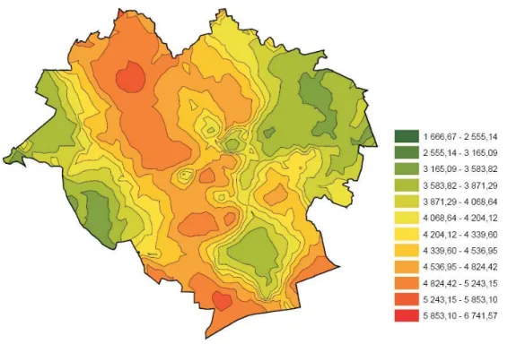
The resulting cartographic presentation (Fig. 4) and a noise map (Fig. 1) sup-port a direct comparison of average prices and noise levels at every point of the analyzed area. 0 500 1000 1500 2000 2500 3000 3500 4000 Lag Distance 0 100000 200000 300000 400000 500000 600000 Nugget effect: error variance: 329320 Spherical model: scale: 267570 length: 2491.23

Fig. 3.Variogram of average unit prices of apartments with the fit theoretical model

Fig. 4.Analysis of the spatial distribution of average apartment prices with the use of

Noise intensity data is not directly related to apartments which can differ sub-ject to their location inside a building. For this reason, it has been assumed that the determined noise level will apply to the entire building. This approach could pose significant problems because various parts of the building could be exposed to different levels of noise. To compensate for that shortcoming, the maximum, minimum and average noise levelLDWNwas determined for each building

contain-ing the analyzed apartments. The performed analyses accounted mostly for maxi-mum noise levels to which the building is exposed.

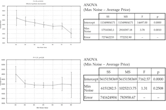
The impact of noise on apartment prices was assessed with the use of the ANOVA test, a statistical method for determining the presence of differences be-tween means in several populations. This method estimates the probability with which the analyzed factors could explain the differences between the observed means in groups. The purpose of the ANOVA test in this study was to verify whether noise levels significantly affect apartment prices. As part of the analysis, the general variance in the dependent variable was divided into inter-group and intra-group variance [1]. When a given type of variance is compared against resid-ual variance, i.e. random error variance (using Snedecor’s F-distribution), the re-sult indicates whether the analyzed factor (noise intensity) significantly affects transaction prices.

F=3.78, p=0.0010 Effective hypothesis decomposition

45 50 55 60 65 70 75

Max Noise Value 3600 3800 4000 4200 4400 4600 4800 5000 5200 F=1.31, p=0.25 30 35 40 45 50 55 60

Min Noise Value 3600 3800 4000 4200 4400 4600 4800 5000 5200 5400 A verage Price A verage Price

Fig. 5.Results of the analysis of variance (ANOVA)

ANOVA

(Max Noise – Average Price)

SS MS F p Intercept 11349804171 11349804171 14697.00 0.0000 Max Noise 17510383,1 2918397.18 3.78 0.0010 Error 727462233 772252.90 – – ANOVA

(Min Noise – Average Price)

SS MS F p

Intercept 5615158369 5615158369 7162.57 0.0000 Min

Noise 6151282.5 1025213.75 1.31 0.2508

The results of the ANOVA test indicate that noise levels contribute to a signifi-cant variation in the unit prices of apartments in Olsztyn (Fig. 5). Maximum noise levels were a significant parameter at the level of 0.001.

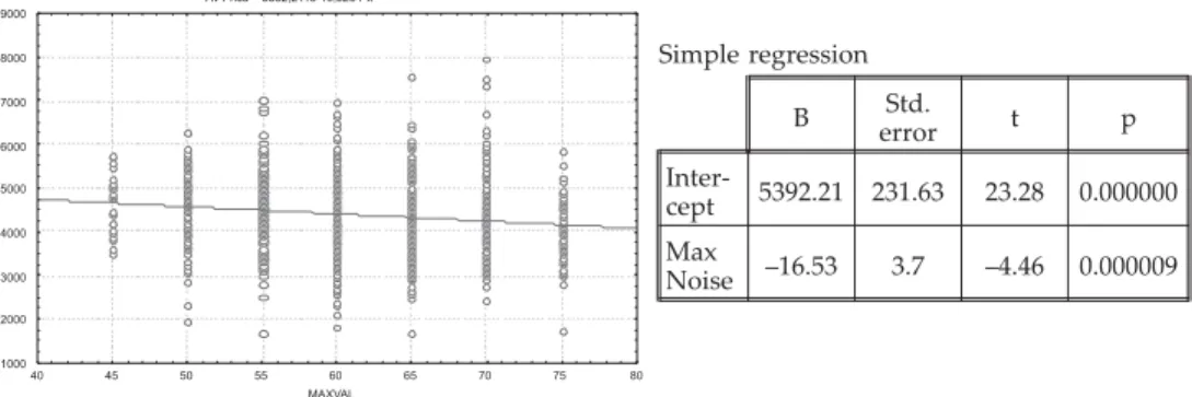
The maximum noise level was the most significant parameter in buildings characterized by varied noise intensity. Pearson’ correlation coefficient between maximum noise intensity and average prices reached –0.135, and it was significant below the level of 0.05. The results of a simple regression analysis suggest that unit prices decrease by PLN 16.53/m2_{per every 1 dB increase in noise intensity}

(Fig. 6).

The value of NSDI was estimated at 0.36%. and it is consistent with the find-ings reported by Nelson [20], Bateman et al. [5] and Theebe [25]. Despite a low co-efficient of determination at 0.19, the analyzed dependency can be assumed to be statistically significant. In our study, we analyzed the data from the entire sur-veyed area. Detailed investigations revealed that a better fit of the model would be obtained if every residential estate in the studied area were analyzed separately.

Preliminary analyses confirm that noise intensity could significantly contribute to variations in the usable value and, consequently, the unit prices of apartments. The studied parameter’s influence could vary subject to individual location.

The spatial distribution of prices is affected by numerous factors, including lo-cation, predominant type of construction, proximity of transport routes and resi-dential safety. Noise intensity is most profoundly manifested on a micro scale, i.e. within a small district or residential estate. For this reason, a geographically weighted regression model can be used to determine spatial correlations in detail. The unit price of an apartment was the dependent variable in the model, whereas the maximum noise level, expressed by indicator LDWN, was the independent variable. The results of the GWR analysis are presented in table 1.

Av Price = 5392,2118-16,5264*x 40 45 50 55 60 65 70 75 80 MAXVAL 1000 2000 3000 4000 5000 6000 7000 8000 9000 A verage Price

Fig. 6.Results of a regression analysis of average prices and maximum noise intensity

Simple regression B Std. error t p Inter-cept 5392.21 231.63 23.28 0.000000 Max Noise –16.53 3.7 –4.46 0.000009

The effect of noise intensity on apartment prices is spatially differentiated, as demonstrated by the slope of the regression line. The spatial distribution of re-gression parameter â1and the fit of the model measured by the coefficient of

de-terminationR2are shown in figure 7.

In regions marked by the lowest noise intensity, the value of coefficient â1 reached –2.917 PLN/dB, and in areas that are most affected by noise, it was equal to –29.206 PLN/dB, which corresponds to NSDI values in the range of 0.07% to 0.67%. The local coefficient of determination ranged from 0.001 to 0.131.

Environmental noise had the greatest influence on real estate prices in the south-eastern parts of Olsztyn which comprise mostly residential estates. In the above area, maximum noise intensity did not exceed 60 dB, excluding apartments

Table 1.General results of the GWR analysis

Intercept (b0) Error (b0) Max val. (b1) Errorb1 LocalR2

Min 4252.98 304.33 –29.206 4.681 0.001

Max 6046.36 850.12 –2.917 14.042 0.131

Average 5391.69 376.08 –15.803 6.030 0.032

Fig. 7.Spatial analysis of the strength of noise effects on prices and the fit of a statistical

in the immediate vicinity of the main street. Noise had a slightly less profound ef-fect on prices in estates situated closer to the city center despite a high degree of spatial variation in noise pollution levels. The above could be attributed to the fact that potential buyers who opt for apartments in downtown Olsztyn are more will-ing to accept the annoyance effects of urban noise.

The spatial distribution of the goodness of fit of the GWR model is similar to that observed in the relationship between noise and prices. The most significant correlations were reported in areas where noise had the greatest impact on real es-tate prices.

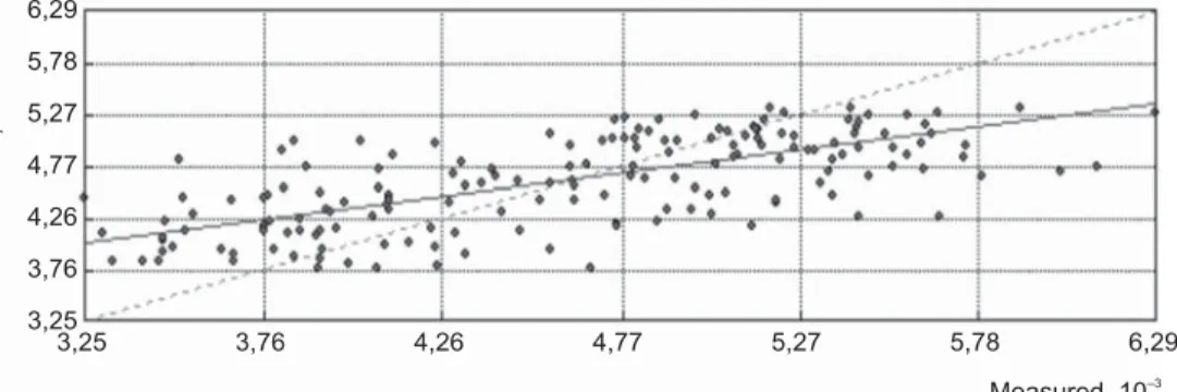
To account for the fact that price data is often incomplete and that transac-tions are unevenly distributed in space, the final map of apartment prices was de-veloped by co-kriging based on the correlations between transaction prices and noise intensity. The resulting map presents the spatial distribution of apartment prices in view of noise levels (Fig. 8). Co-kriging methods supported the estima-tion of average prices in areas that are covered by the noise map but where no transactions were registered. This approach improved the fit of the interpolated space to the existing data.

The differences between the results of kriging and co-kriging interpolation are significant only when the main variable (transaction price) is significantly spatially correlated with the additional variable. Therefore, the most reliable results are noted in areas where the GWR model best fits market data. It should be noted,

Fig. 8.Comparison of interpolation results by ordinary kriging and co-kriging with the

however, that real estate prices are not always easy to model, and the results can be burdened with relatively high error. The relationship between transaction prices and the modeled values is illustrated in figure 9.

6. Conclusions

The results of this study indicate that road traffic noise significantly impacts the usable value and, consequently, the prices of real estate. The presented meth-odology supports the determination of the quantitative effects of environmental noise on apartment prices and the generation of maps illustrating the influence of noise on the spatial distribution of prices. The performed analyses validate the usefulness of selected geostatistical methods in studies evaluating the effect of en-vironmental factors on local real estate markets. The applied GWR models sup-port the assessment of the spatial variation in noise effects on prices. The use of co-kriging methods for interpolating average prices in view of noise levels contrib-utes to the accuracy of maps of average real estate prices.

The information on the spatial variation in noise effects on prices provides valuable inputs for the initiation of measures to mitigate noise and prevent a de-crease in the usable value and prices of real estates.

References

[1] Aczel A.: Complete Business Statistics. 2nd ed., Richard D. Irwin Inc., Burr Ridge, Illinois 1993.

[2] Andersson H., Jonsson L., Ögren M.:Property Prices and Exposure to Multiple Noise Sources: Hedonic Regression with Road and Railway Noise. Environmental Resource Economic, vol. 45, 2010, pp. 73–89.

Fig. 9.Relationship between transaction prices and values obtained from a theoretical

[3] Anselin L.:Advances in Spatial Econometrics.Springer, Berlin 2004.

[4] Basu S., Thibodeau T.G.: Analysis of spatial autocorrelation in housing prices. Journal of Real Estate Finance and Economics, 17, 1998, pp. 61–85.

[5] Bateman I., Day B., Lake I., Lovett A.:The Effect of Road Traffic on Residential Property Values: A Literature Review and Hedonic Pricing Study. Study for Scot-tish Executive Development, 2001.

[6] Blanco J.C., Flindell I.:Property prices in urban areas affected by road traffic noise. Applied Acoustics, vol. 72, 2011, pp. 133–141.

[7] Brandt S., Maening W.:Road noise exposure and residential property prices: Evi-dence from Hamburg. Transportation Research, Part D 16, 2011, pp. 23–30. [8] Charlton M., Fotheringham S.: Geographically Weighted Regression. National

Centre for Geocomputation, Maynooth (Ireland) 2009.

[9] Davis J.C.: Statistics and Data Analysis in Geology. John Wiley & Sons, New York 1986.

[10] Dubin R.A.: Predicting House Prices Using Multiple Listings Data. Journal of Real Estate Finance and Economics, vol. 17, no. 1, 1998, pp. 35–59.

[11] Haining R.:Spatial Analysis of Regional Geostatistics Data. Cambridge Univer-sity Press, 2003.

[12] Huang J.C., Palmquist R.B.:Environmental Conditions, Reservations Prices, and Time on the Market for Housing. Journal of Real Estate Finance and Economics, vol. 22, no. 2/3, 2001, pp. 203–219.

[13] Hughes W.T., Sirmans C.E.:Traffic Externalities and Single-Family House Prices. Journal of Regional Science, vol. 32, no. 4, 1992, pp. 487–500.

[14] Ismail S., Iman A., Kamaruddin N., Mohd H.: Spatial autocorrelation in hedonic model: Empirical evidence from Malaysia. International Real Estate Sym-posium “Benchmarking, Innovating and Sustaining Real Estate Market Dy-namics”, Kuala Lumpur (Malaysia) 2008.

[15] Kim K.S., Park S.J., Kweon Y.: Highway traffic noise effects on land price in an urban area. Transportation Research, Part D 12, 2007, pp. 275–280.

[16] Kubiak J.:Kartograficzne sposoby prezentacji zjawisk akustycznych na przyk³adzie wybranych map tematycznych. [in:] Sirko M., Cebrykow P. (red.),Prace i studia kartograficzne, Oddzia³ Kartograficzny PTG, Lublin 2007, pp. 101–109. [17] Kulczycki M., Ligas M.: Zastosowanie analizy przestrzennej do modelowania

danych pochodz¹cych z rynku nieruchomoœci. Studia i Materia³y Towarzystwa Naukowego Nieruchomoœci, vol. 15, nr 3–4, 2007, pp. 145–154.

[18] Kwiecieñ J., Szopiñska K., Sztubecka M.: Problem ochrony przed ha³asem na terenach zurbanizowanych na przyk³adzie miasta Bydgoszcz. Ekologia i Technika vol. XVIII, nr 4, 2010, pp. 205–212.

[19] Leuangthong O., Khan K.D., Deutsch C.V.: Solved Problems in Geostatistics. John Wiley & Sons, 2008.

[20] Nelson J.P.: Highway Noise and Property Value: A Survey of Recent Evidence. Journal of Transport Economics and Policy, vol. 16, no. 2, 1982, pp. 117–138. [21] Pace R.K., Barry R., Sirmans C.F.: Spatial Statistics and Real Estate. Journal of

Real Estate Finance and Economics, vol. 17, no. 1, 1998, pp. 5–13.

[22] Schkade D.A., Payne J.W.: How People Respond to Contingent Valuation Ques-tions. A Verbal Protocol Analysis of Wilingness to Pay for an Environmental Regu-lation. Journal of Environmental Economics and Management, vol. 26, no. 1, 1994, pp. 88–109.

[23] Smith V.K., Mansfield C.:Buying Time: Real and Hypothetical Offers. Journal of Environmental Economics and Management, vol. 36, no. 3, 1998, pp. 209–224.

[24] Stach A.: Analiza i modelowanie struktury przestrzennej. [in:] Zwoliñski Z. (red.), GIS – platforma integracyjna geografii, Bogucki Wydawnictwo Nauko-we, Poznañ 2009, pp. 115–144.

[25] Theebe M.:Planes, Trains and Automobiles: The Impact of Traffic Noise on House Prices. Journal of Real Estate Finance and Economics, vol. 28, 2004, pp. 209–234.

[26] Tu Y., Sun H., Yu S.:Spatial autocorrelations and urban housing market segmenta-tion. Journal of Real Estate Financial and Economy, vol. 34, 2007, pp. 385–406.

[27] Wackernagel H.:Cokriging versus kriging In regionalized multivariate data analy-sis.Geoderma, vol. 62, 1994, pp. 83–92.

[28] Weber D., Englund E.J.: Evaluation and comparison of spatial interpolators. Mathematical Geology, vol. 24, no. 4, 1992, pp. 381–391.

[29] Wilhelmsson M.: The Impact of Traffic Noise on the Values of Single-family Houses. Journal of Environmental Planning and Management, vol. 43, no. 6, 2000, pp. 799–815.

[30] Kucharski R. (red.):Wytyczne opracowania map akustycznych. Instytut Ochrony Œrodowiska, Warszawa 2006.

[31] Zimmerman D., Pavlik C., Ruggles A., Armstrong M.P.:An experimental com-parison of ordinary and universal kriging and inverse distance weighting. Mathe-matical Geology, vol. 31, no. 4, 1999, pp. 375–390.