Service Functions Technology Overview

(1)

55

3

Service Functions Technology Overview

Worthless.

—Sir Airy, 1842, regarding the analytical engine [1].

The following sections discuss basic Ethernet concepts and the Ethernet service elements in each of the service function groups:

• Service logic defi ning connectivity, fl ow defi nition, and interface types; • Service transport technology;

• Service reliability and protection; • Service quality of service; • Service performance;

• Service management and verification;

• Interconnectivity between the customer and providers networks.

3.1 Service

Logic

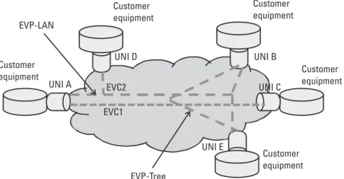
Service logic defines the way UNIs are interconnected (i.e., the logic of the service, the flow of the traffic, and the connectivity between edge of the services or UNIs). More importantly, each type of Ethernet service has certain proper-ties that define how the service operates. Thus, each service has distinguishing characteristics and is targeted for the specific tasks (read service). Table 3.1 sum-marizes the types of Ethernet services.

(2)

3.1.1 E-Line Service

The E-line service is a service in which each EVC has associated exactly one pair of UNIs. The E-line service maybe port-based (EP-line) or virtualized (EVP-line). In the Ethernet private line (EPL) service, each UNI has associated only one EVC. Thus, each UNI is associated only with one other UNI. All service frames [4] that ingress at one UNI should be transported to the other UNI. The E-line EPL service architecture is depicted in Figure 3.1 and the related EVC UNI map in Table 3.2

In the EVPL E-line service, each UNI may have associated multiple EVCs and multiple UNIs. However, one EVC is still associated with a pair of UNIs. Each EVC is a considered a separate flow and may have different characteristics defined in its EVC profile. Subsequent sections will detail these aspects of the EVCs. All frames ingressing at one UNI into one EVC will egress at the other UNI associated with this EVC. Frames that are not associated with a specific

Table 3.1 MEF Ethernet Services [2] Service Type [3] Port-Based Service

VLAN-Based (Virtualized Service) E-line (point-to-point [p2p] EVC) Ethernet private line (EPL) Ethernet virtual private line

(EVPL) E-LAN (multipoint-to-multipoint

[mp2mp] EVC)

Ethernet private LAN (EP-LAN) Ethernet virtual private LAN (EVP-LAN)

E-tree (rooted multipoint [p2mp] EVC)

Ethernet private tree (EP-TREE) Ethernet virtual private tree (EVP-tree)

Figure 3.1 EP-line port-based service.

Table 3.2

EVC UNI Map for the EP-Line Service

EVC UNIs

(3)

EVC should not be admitted to this EVC. This condition achieves a virtual [5] separation of the flows in each EVC; hence the name—virtual connection. This separation property resembles the dedicated physical circuit of TDM technol-ogy. However, in the case of EVC the circuit, the connection is virtualized (i.e., logical, not physical). The EVPL service architecture is depicted in Figure 3.2.

The EVC-UNI map [6] for the EVPL service contains also (as EPL) one EVC two UNIs as in Table 3.3.

3.1.2 E-LAN Service

The E-LAN services associate one EVC with multiple UNIs. The EP-LAN ser-vices can be port-based (EP-LAN) or virtualized (EVP-LAN). E-LAN serser-vices are depicted in Figure 3.3 and Figure 3.4.

The EP-LAN service has different operational properties from EVP-LAN services that need to be understood by the customer buying this service. In the EP-LAN services frames entering one of the UNIs will be transferred to another UNI on this EVC based on the frames MAC addresses. The network support-ing such service must allow frames to be switched to the specific destination egress UNI based on the frame’s MAC DA. In the Ethernet technology the function allowing this switching is called bridging. How and where the bridg-ing function is implemented in the network is dependent on the underlybridg-ing

Table 3.3 EVC Map for the EVPL Service EVC UNIs

EVC1 UNI A UNI B EVC2 UNI A UNI C EVC3 UNI A UNI D Figure 3.2 EVPL service.

(4)

Ethernet technology, and it should be of lesser concert to the customer buying MEBH service.

The EP-LAN service (Figure 3.3) is a port-based service, which means that all frames (tagged or untagged) arriving at a UNI may be transported to their destinations, if permitted to enter EVC. There is only one EVC associated with the UNIs. On Figure 3.3 the EP-LAN EVC connects four UNIs. In this Figure 3.3 EP-LAN service.

(5)

service, service frames can travel from any UNI to any UNI in the EVC. Thus, broadcast, multicast, and unknown unicast (BMU) frames are sent to all UNIs. Known unicast frames will be sent to their specific destinations, once these are learned. The EP-LAN service, as with all bridged services, requires careful engineering to prevent BMU [7] storms. The EVC UNI map for the service in Figure 3.3 is illustrated in Table 3.4.

The E-LAN service offered over a multiplexed UNI, denoted as the EVP-LAN service, is depicted in Figure 3.4.

The EVP-LAN service is a virtualized EP-LAN service (i.e., the service allows the coexistence of different EP-LAN-EVCs on the same UNI). As pre-sented in Figure 3.4 on UNI A and UNI D, there are two EVP-LANs. Each EVP-LAN has a unique EVC associated with it. Most of the properties of the EP-LAN service are preserved in the EVP-LAN service. Service frames coming to the UNI from the customer side will be mapped to the specific EVP-LAN EVC based on the EVC map. Frames not present in the EVC map will be dropped. Untagged frames, if no mapping specifies the EVC on which they could be transported, will be dropped. The EVP-LAN service is a port-multi-plexed service; more than one EVC may exist on one port, and one EVP-LAN EVC UNI map is illustrated in Table 3.5.

The EVP-LAN can be combined with any other virtualized service as depicted in Figure 3.5. In Figure 3.5 the EVP-LAN service coexists with EVPL on UNI A. As in the EP-LAN service, in the EVP-LAN service UNIs belong-ing to the specific EVP-LAN can send frames (BMU) to any of the UNIs par-ticipating in the EVP-LAN. On the specific UNI only frames with the VLAN IDs that are associated with the EVP-LANs associated with this UNI (via EVC maps) will be transported. All other frames as well as untagged frames will be dropped, unless special provisions are made to map such frames to the specific EVP-LAN EVC.

Table 3.4 EP-LAN EVC UNI Map EVC UNIs

EVC1 UNI A, UNI B, UNI C, UNI D

Table 3.5 EVP-LAN EVC UNI Map EVC UNIs

EVC1 UNI A, UNI C, UNI E EVC2 UNI A, UNI B, UNI D EVC3 UNI D, UNI C, UNI F

(6)

In combining the diffident virtualized service, like EVP-LAN and EVPL, on a single UNI the properties of the EVCs are preserved. This means that the traffic in each EVC is separated, each EVC is either p2p or mp2mp, and each EVC may have different attributes. The EVC UNI maps define which frames are mapped to which EVC and which are dropped. Each EVC is also a separate broadcast domain containing the BMU traffic. The EVC UNI map for the EVP-LAN and EVPL service is presented in Table 3.6.

3.1.3 E-Tree Service

The E-tree is the third generic Ethernet service supported in MEF Ethernet net-works. As with other services, the E-tree service maybe port-based (EP-TREE) or virtualized (EVP-TREE). The EP-tree service is represented in Figure 3.6.

In the EP-tree service one UNI is defined as a root of the tree, and other UNIs are defined as leaves. The root UNI can send any traffic to any of the leaves. The leaf UNIs can send traffic only to the root UNI. Thus, leaves cannot communicate between themselves. In such a service the BMU traffic is greatly reduced, as the traffic of such type between leaves UNIs is blocked. The root UNI has therefore a critical role in the EP-tree service, as it is only through

Table 3.6

EVP-LAN and EVPL Service EVC UNI Map

EVC UNIs

EVC1 UNI A, UNI C EVC2 UNI D, UNI F EVC3 UNI A, UNI B, UNI E

(7)

this UNI that leaf UNIs can communicate. The EP-tree EVC UNI map is presented in Table 3.7

To increase the resiliency of the service, one may implement the EP-tree with two or more roots (as in Figure 3.7). In such a construct, called multiroot tree, if the primary root UNI fails the other root UNI can take over the func-tions of the primary root, preserving the continuity of service.

As with all Ethernet services, the EP-TREE service can be virtualized as the EVP-tree. The EVP-tree construct allows coexistence of multiple virtualized Ethernet services on the same UNI as illustrated in Figure 3.8; one could design multiplexed EVP-trees or a combination of other virtualized services. Table 3.8 presents the EVC UNI map for this service.

The EVP-tree services preserve the E-tree properties and behavior (with the exception of the all-to-one bundling) and can be, as with other multiplexed services, combined with other virtualized Ethernet services. An example of such a combination of virtualized services is presented in Figure 3.9. The service EVP-LAN as 2 is implemented on the same UNIs as the EVP-tree EVC-1. Table 3.9 provides the EVC UNI map for the service. Other combinations of virtualized services are also possible.

Table 3.7 EP-Tree EVC UNI Map EVC UNIs

EVC 1 UNI A (root), UNI B (leaf), UNI C (leaf), UNI D (leaf) Figure 3.6 EP-tree service.

(8)

Figure 3.7 Multiroot EP-tree.

Figure 3.8 EVP-tree service.

Table 3.8 EVP-Tree EVC UNI Map EVC UNIs

EVC 1 UN A (root), UNI B (leaf), UNI C (leaf), UNI E (leaf) EVC-2 UNI D (root), UNI C (leaf), UNI E (leaf)

(9)

3.1.4 Services in Multiprovider Architecture

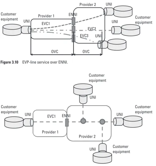
The canonical Ethernet service types (E-LAN, E-tree, and E-line) are also avail-able in the multiservice provider architecture. The definitions of the services do not change. What changes is the detailed design of the service, depending on the location of specific OVCs and UNIs. Next, we present examples of two canonical services, E-line and E-LAN, from the previous section in the multi-service provider environment. Figure 3.10 presents the EVP-line multi-service over the ENNI, and Figure 3.11 presents the EVP-LAN service over ENNI. The presented services are deployed over two service providers. But they can be in a similar way extended over multiple providers. The design of the multiprovider service is, or should be, transparent to the customer of the MEBH service. The definitions of the ENNI related service attributes is a responsibility of the pro-viders of the OVCs.

The service in Figure 3.10 uses three EVPL EVCs. The EVCs span two service providers; each EVC is therefore composed of two OVCs. The mode by which the service providers interface with each other should be transparent to the customer. The providers would interface with a single ENNI rather than with three, one per EVC, as depicted in Figure 3.10. Each EVC is p2p. They Figure 3.9 EVP-LAN and EVP-tree coexisting on the same network.

Table 3.9 Mixed EVC EVC UNI Map EVC UNIs

EVC1 UNI A (root), UNI B (leaf), UNI C (leaf), UNI E (leaf) EVC2 UNI A, UNI D, UNI B, UNI E

(10)

share on the near side one UNI, but each one has a different UNI on the far side. Each EVC may have different attributes.

Figure 3.11 represent the EP-LAN service over the ENNI. The service is offered by two providers. The providers are interfacing with a single ENNI.

The service characteristics of the specific service type should not change, re-gardless of whether the service is provided over the single or multiple providers [8].

3.1.5 Layer 2 Control Protocol (L2CP)

L2CP filtering rules define the characteristics of the EVC and UNI, and, as they are the function of the service logic, they are discussed in this section.

Figure 3.10 EVP-line service over ENNI.

(11)

The Layer 2 Control Protocol (L2CP) term refers to the traffic flows that carry the information about the status of services or network [9]. The L2CP frames have a MAC destination address (DA) within the range 01-80-C2-00-00-00 through 01-80-C2-00-00-0F and 01-80-C2-00-00-20 through 01-80-C2-00-00-2F. The treatment of L2CP frames is addressed by standard IEEE 802.1ad-2005 Provider Bridge. Three actions are defined for the L2CP frame on the UNI: tunnel, peer, or discard.

Discard means that the UNI will discard ingress L2CP frames [10]. Peer means that the MEN will actively participate with the protocol [11]. For ex-ample, LACP/LAMP, link OAM, port authentication, and E-LMI might be peered by the UNI. Tunnel means that service frames containing the protocol will be transported across the MEN to the destination UNI(s) without change [12]. What follows is a simplified description of the L2CP processing rules as stated in MEF 6.1.1 [13].

The MEF 6.1.1 is mostly concerned with the L2CP frames falling within the 01-80-C2-00-00-00 to -0F MAC DA. The control protocols with their Ethertype using these MAC DAs are listed in Table 3.10.

These L2CP protocols are standard protocols defined by the standard fo-rums with well-specified properties and with applications to the Ethernet ser-vices in general, not for the specific platform. One word of caution: sometimes the boundary between the standard protocol and the vendor-specified protocol may be a bit fuzzy. Some vendors created protocols that later on became stan-dardized (like E-LMI).

The action (tunnel, peer, or discard) for each L2CP service frame will be decided using a two-step logic based, first, on the frame’s MAC DA and then on the frame’s Ethertype and subtype or LLC code. The logic for processing of the L2CP service frames is presented in the flow chart in Figure 3.12.

Thus, if for the specific frame, based on the frame’s MAC DA, Table 3.11 mandates tunneling, the frame must be tunneled. If for this frame, based on

Table 3.10

L2CP Control Protocols in MEF 6.1.1 Protocol Type Ethertype/Subtype

STP/RSTP [14]/MSTP [15] NA [16]

PAUSE [17] 0x8808

LACP|LAMP 0x8809/01|02

Link OAM 0x8809/03

Port authentication [18] 0x888E

E-LMI [19] 0x88EE

LLDP [20] 0x88CC

PTP Peer-Delay [21] 0x88F7

(12)

the frame’s MAC DA, Figure 3.12 mandates peer or discard, the action for the L2CP frame is based on the frame’s protocol type (defined by the Ethertype and Figure 3.12 L2CP processing steps [23].

Table 3.11 L2CP Processing—Step 1 Destination MAC Address

L2CP Action for EPL, EP-Tree, EP-LAN

L2CP Action for EVPL, EVP-Tree, EVP-LAN

01-80-C2-00-00-00 [24] Must tunnel Must not tunnel (additional requirements may apply as per the specifi c service type) 01-80-C2-00-00-01 through

01-80-C2-00-00-0A

Must not tunnel (additional requirements may apply as per the specifi c service type)

01-80-C2-00-00-0B Must tunnel 01-80-C2-00-00-0C Must tunnel 01-80-C2-00-00-0D Must tunnel

01-80-C2-00-00-0E Must not tunnel (additional requirements may apply as per the specifi c service type)

(13)

subtype or LLC code) and is specified in subsequent, service specific tables— Table 3.12 and Table 3.13.

Outside of this group of protocols there is a whole gamut of protocols whose treatment is not defined so precisely. These protocols fall into the cat-egory of vendor-specific protocols, and their processing on the UNI will differ from platform to platform. For the detailed account of the L2CP processing as specified by MEF, the reader should consult the standard.

The processing of the L2CP traffic on the ENNI is the subject of the ongoing work in MEF (as of 2013).

3.2 Service

Transport

3.2.1 Ethernet Technology

Ethernet technology is specified by the IEEE standards 802.3 and 802.1. The IEEE 802.3 [25] defines the technology that supports the IEEE 802.1 [26] ar-chitecture. In rare cases, a network engineer designing the Ethernet service deals with the Ethernet technology only; usually the Ethernet service is offered in the complex networking environment. Thus, to fully understand the environ-ment in which the Ethernet service is delivered, it is necessary to provide even a limited view of the networking context of the Ethernet services. The selection of the technology over which Ethernet service is delivered will have a definite

Table 3.12

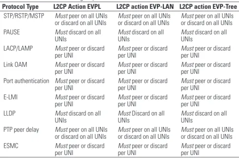
L2CP Processing Requirements for Virtualized Ethernet Services

Protocol Type L2CP Action EVPL L2CP action EVP-LAN L2CP action EVP-Tree STP/RSTP/MSTP Must peer on all UNIs

or discard on all UNIs

Must peer on all UNIs or discard on all UNIs

Must peer on all UNIs or discard on all UNIs PAUSE Must discard on all

UNIs

Must discard on all UNIs

LACP/LAMP Must peer or discard per UNI

Must peer or discard per UNI

Link OAM Must peer or discard per UNI

Port authentication Must peer or discard per UNI

E-LMI Must peer or discard per UNI

LLDP Must discard on all UNIs

Must Discard on all UNIs

PTP peer delay Must peer on all UNIs or discard on all UNIs

Must peer on all UNIs or discard on all UNIs ESMC Must peer or discard

per UNI

(14)

impact on the services—it may limit its service features or allow for its smooth growth and evolution.

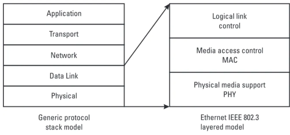
The context of networking technologies is usually presented in a form of protocol stack, or functional layers as seen in Figure 3.13 [27]. The protocol stack is an abstract representation of networking protocols and their physical realizations.

Each layer in the stack has a set of defined functions and interfaces, or service access points (SAPs), to the layers above and below. Layers communi-cate only through these interfaces by passing up or down the stack PDUs. The

Table 3.13

L2CP Processing Requirements for Port-Based Ethernet Services

Protocol Type L2CP Action EPL L2CP Action EP-LAN L2CP Action EP-Tree STP/RSTP/MSTP Must peer on all UNIs or

discard on all UNIs

Must peer on all UNIs or discard on all UNIs PAUSE MUST discard on all

UNIs

LACP/LAMP Must peer or discard per UNI

Link OAM Must peer or discard per UNI

Port authentication Must peer or discard per UNI

E-LMI Must peer or discard per UNI

LLDP Must peer or discard per UNI

PTP peer delay Must peer or discard per UNI

Must peer on all UNIs or discard on all UNIs ESMC Must peer or discard

per UNI

(15)

isolation of layers allows implementation of the functions on the specific layer independent of other layers.

We can briefly characterize each of the layers as having the following functions. Application layer functions are responsible for user applications and interfaces. The transport layer is responsible for flow control among other func-tions. The network layer is responsible for packet forwarding and routing. The data link layer is responsible for packet forwarding between network entities. The physical layer is responsible for physical (hardware) encoding and decoding as well as transmission management.

The IEEE Ethernet standards define physical and logical aspects of Ether-net technologies in the data link and physical layers defined as in Figure 3.14. The Ethernet service uses facilities and functions of the data link layer—layer 2. That is why Ethernet service is called a layer 2 service.

For the purpose of this book it is sufficient to provide only the brief char-acteristics of each of the IEEE 802.3 layers. The physical layer defines how the bits are transfer over the physical (wireline or wireless) media. It also specifies the physical connectivity or interfaces on the devices connected to the Ethernet. The data link layer from the generic protocol stack is composed of the media access control (MAC) and logical link control (LLC) sublayers. The MAC sub-layer supports data encapsulation, media access management and transmission control, and other functions. The LLC layer primarily supports flow control and multiplexing or frames, and it provides the interface to upper protocol lay-ers [28].

Native Ethernet uses the IEEE Ethernet protocol stack—physical and data link layers. In carrier networks, however, Ethernet service may be pres-ent in several locations in the stack depending on the design of the service and transport. In addition, the Ethernet service context may be different in the

(16)

access, handoff, and core segments of the MEBH service as depicted in Figure 3.15.

Figure 3.16 presents the network design in which the Ethernet service is delivered over the MPLS [29] transport network over the Ethernet transport. The service provider will interact only with the lower Ethernet layer, in most cases. The provider has to be aware of the design (or a composition) of the transported frame, as quite often unexpected problems in the service may have a root cause in the lower layer design. Of course, the MPLS protocol stack in Figure 3.16 is greatly simplified. The detailed protocol stack would list all of the MPLS components and complexities of transport.

The service architect must be cognizant of the Ethernet frame context for many reasons. One is that the networking technology in which Ethernet services are embedded impacts the way the services behave—among aspects impacted are performance, resiliency, fault propagation, restoration, and QoS. Why is that so? It is because each technology has its own control plane, manage-ment plane, and signaling plane methods and resources. And these specificities must be recognized to fully understand the end-to-end service. The following sections introduce the most common networking technologies in which the Ethernet service is delivered.

3.2.2 Transport Technologies

The networking technologies employed with Ethernet service are presented in Figure 3.17. Ethernet may be delivered over wireline or wireless media. We leave out the wireless technology from further discussion and focus on

(17)

line. Wired technology may support coaxial, copper, or fiber media. Over these media one may use TDM, SONET/SDH, switching, and PON technologies. Provider backbone bridging (PBB) and multiprotocol label switching (MPLS) provide layer 2 transport functions for the Ethernet technology mediating often between the lower transport layers and the Ethernet service. Thus, they are not equivalent to TDM, SONET/SDH, and PON.

The following descriptions of different technologies are far from being comprehensive and are intended only to highlight the most important features relevant, in author’s view, to the MEBH service design, meaning the support for Ethernet service attributes. Such an approach, by its nature, leaves out vast amount of technical details and introduces simplifications in representing oth-erwise complex technologies—reader beware!

3.2.2.1 Ethernet over SONET/SDH (EoS)

EoS refers to the Ethernet service supported over the synchronous optical net-work (SONET/SDH)/ synchronous digital hierarchy (SDH) transport tech-nologies. SONET is predominantly North American standard. SDH is used outside of North America. In the EOS architecture, Ethernet frames are sent Figure 3.16 Ethernet Service over MPLS.

(18)

over the SONET/SDH link encapsulated into the generic framing procedure [30] (GFP) block that maps the asynchronous Ethernet flows into the synchro-nous the SONET/SDH stream. GFP mapping is a generic mapping procedure that can be used to map packets into the SONET/SDH frames. The mapping drops the Ethernet frame control fields, improving the efficiency of the trans-port. The SONET/SDH technology provides the guaranteed bandwidth and robust protection mechanisms.

In SONET/SDH the main transport is implemented using the multiples of STS-1 containers of roughly 50 Mbps. The actual payload capacity is lower. For fined granularly (less than STS-1) one can use VT1.5 containers of 1.6 Mbps. The combinations of STS-1 or VT1.5 containers are called virtual con-catenation groups (VCG) with STS1 combinations called high-order VCGs and with VT1.5 called low-order VCG. Examples of rates offered by EoS ser-vice are provided in Table 3.14.

The Ethernet bandwidth [32] or the actual Ethernet layer (layer 2) band-width depends on the packet size (service frame size). As the Ethernet over SONET/SDH uses GFP encapsulation (12 bytes), the actual payload band-width is reduced by the overhead percentage. For example, STS1 50.112 Mbps payload rate has to be reduced for 512 bytes frames by 512/(512+12) = 0.977 or 97.7 percent, giving 48.77 Mbps Ethernet or service frame throughput.

EoS guarantees high QoS quality of the service (no overprovisioning), ro-bust protection architectures, roro-bust OAM plane, and very fast (within 50 ms) recovery times. It is suited for EPL and EVPL (point-to-point) Ethernet servic-es. At present (2013), the SONET/SDH technology is going out of favor. The main reasons for this are lack of bandwidth flexibility that is available with layer 2 technologies, relatively high cost of the infrastructure, no support for classes of service, lesser efficiency as compared to packet-based technologies, and no support for overprovisioning. All these limitations should not prevent anyone from seeing EoS technology service as delivering reliable and matured service.

Table 3.14

Examples of SONET/SDH Payload Rates SONET/SDH Frame Format/ Optical Carrier Level [31] SDH Level and Frame Format Payload Bandwidth (Mbps) STS-1/OC-1 STM-0 50.112 STS-3/OC-3 STM-1 150.336 STS-12/OC-12 STM-4 601.344 STS-48/OC-28 STM-16 2,405.376 STS-192/OC-192 STM-64 9,621.504 STS-768/OC-768 STM-256 38,486.016

(19)

EOS technology can be used both in the access and core transport seg-ments of the MEBH service in a variety of topologies (e.g., point-to-point or ring). EoS technology is defined by ITU (SDH) and ANSI (SONET/SDH) standards [33].

3.2.2.2 Ethernet over Cable

EoCable or EthernetoHFC refers to the technology specified by data over cable service interface specification (DOCSIS) [34] for high-speed data transfer over the hybrid fiber-coaxial (HFC) media, which combines optical fiber and coaxial cable. Data signal in HFC technology is encoded over the radio frequency. The data signal is converted into the modulated RF signal and back by the modem device at the customer premises and in the head-end equipment on the other end, respectively. Cable industry typically uses 42–750-MHz RF range, 5–42 MHz for upstream data, and 54–860 MHz for downstream transmission as 6-MHz wide channels. A single 6-MHz channel can support multiple data stream or multiple users with layer 2 (LAN) protocols. Different modulation techniques are used, including quadrature phase shift keying (QPSK) upstream and quadrature amplitude modulation (QAM 64-256) downstream.

Management of different traffic flows is provided with QoS features in-troduced in DOCSIS 1.1. Depending on the DOCSIS release, the throughput (maximum usable throughput without the overhead) may range from 38 Mbps per channel or multiples of it (n × 38 Mbps) in DOCSIS 3.0 downstream to 27 Mbps or multiples of it (n × 27 Mbps). No maximum number of channels (n) is defined. The EoHFC network has a tree topology. Thus, the capacity of the connection is shared among the users. The amount of bandwidth available to the user depends on many factors, among them the number of users, type of traffic, and noise in the cable plant.

3.2.2.3 Ethernet over Wavelength Division Multiplexing (EoWDM)

Ethernet over WDM is a catch term that includes Ethernet transport over opti-cal technologies such as EoOTU, EoDWDM, and Ethernet over fiber (EoF). Ethernet over optical transport network (OTU [35]) uses a new technology defined to optimize the transport of multiple service over the DWDM me-dia. The OTU technology is specified in two ITU standards, ITU G.706 and G.798. It is referred to quite often as a digital wrapper, as it allows the transport of Ethernet, video, SONET/SDH, fiber channel, and others over the common transport unit (OTU) at different speeds ranging from 2.48 Mbps to 100 Mbps (OTU-1 at 2.7 Gbps, OTU-2 at 10.7 Gbps, OTU-3 at 43 Gbps, or OTU-4 at 112 Gbps). The OUT rates are provided in Table 3.15.

The OTU technology offers several advantages such as multiplexing of the client signals, improving the bandwidth efficiency, transparent encapsula-tion of a client signal (Ethernet traffic is encapsulated in to the GFP or GFP-T

(20)

frame), OAM facilities, and 50 msec restoration of transmitted signal. It is es-sentially point-to-point technology.

EoF refers to the Ethernet technology delivered over optical fiber in native format in the variety of interface media and fiber connector options—mul-timode and single mode fiber with a variety of speeds such as Fast Ethernet, 1GiGE, 10 GiGe, and higher.

EoDWDM refers to Ethernet over dense wavelength division multiplex-ing (DWDM) or packet-based transport technology over DWDM. EoDWDM uses OTU wrapping, offering more efficient use of the available bandwidth in comparison to TDM technology. DWDM technology extends from access to the core. By accommodating Ethernet in its native format and with combing of the layer 2 features, it allows for better grooming of traffic by mapping layer 2 flows directly into wavelengths. Additional advantages such as end-to-end man-agement, monitoring, and reducing the complexity of equipment presents the EoDWDM as a less costly and more efficient alternative to the other transport solutions.

3.2.2.4 Ethernet over DSL

Digital subscriber loop (DSL) is a technology that adapts the existing copper-based connections for high-speed data access. The current DSL speeds are reaching past 100 Mbps. The limitation of the technology is its dependence on the distance. As the distance from the head-end office to the customer end point increases, the capacity diminishes significantly. Another feature of the DSL technology is its asymmetry, in particular in earlier released versions. High-end DSL speeds are supported over 10–14Kft, with the maximum speed supported over < 10 Kft distance from the CO. The DSL may reach up to 24 Kft but with significantly reduced bandwidth. DSL bandwidth dependency on the distance is heavily dependent on DSL technology. See Table 3.16 for details of DSL transport.

Table 3.15 OTU Rates and Client Signals

OTU Type

OTU Rate (Gbps)

OTU Payload

Rate (Gbps) Client Signals

OTU1 2.6661 2.48832 STM-1/OC-3, STM-4/OC-12, STM-16/OC-48, GbE,

OTU1e 11.049 10.3215 10GbE LAN

OTU2 10.709 9.9953 STM-64/OC-192, 10GbE WAN, 10GbE LAN (GFP),

OTU2e 11.095 10.356 10GbE LAN

OTU3 43.018 40.150 STM-256/OC-768, 40GbE OTU4 111.80997 104.35597 100GbE

(21)

3.2.2.5 Ethernet over Passive Optical Networks (EoPON)

EoxPON technology refers to the class of access technologies called passive ac-cess technologies. The name comes from the use of the passive optical splitters in the network that enable the use of a single laser for several subscribers. The splitter distributes the signal among customer connections downstream (toward the customer) toward the optical network termination (ONT) unit at the cus-tomer premises. Upstream, the ONT uses the allocated time slots (TDM). The EoxPON technology has several variants including Ethernet-PON (EPON) [37], gigabit (GB) PON (GPON), 10-GB Ethernet PON (10GEPON) [38], or wave-division multiplex PON (WDM-PON). Prevailing installations are that of GPON technology [39]. Current GPON technology offer 2.5 Gbps toward the customer and 1.25 Gbps upstream. With a 32-fold splitter, this potentially may offer the up to 78 Mbps downstream and 39 Mbps upstream. The EPON technology may deliver the service over a 20-km range and with different splitters (16-fold or less), and the bandwidth to the customer may be increased even to 1 Gbps.

3.2.2.6 Ethernet over TDM

EoTDM refers to the Ethernet over TDM n × T1(DS1)/E1 (bonded T1), T3(DS3) (45 Mbps), or its derivatives. This technology is sometimes referred to as Ethernet over copper (EoC). The EoTDM is delivered over the twisted pair cable. A T1 circuit delivers 1.544 Mbps. With bonded technology (which essentially allows aggregating multiple T1 circuits, augmenting the available bandwidth in multiples of T1), one may bond up to eight T1s offering 12 Mbps. Above eight T1s, the bonding becomes less economic. Above 40–50 Mbps, it is more cost-efficient to move to fiber from copper-based technology. EoTDM is precisely the technology from which mobile providers are migrat-ing. As a reminder, T1 and similar technologies haven proven to be outage

Table 3.16 Selected DSL Technologies [36]

Family ITU Name Ratifi ed Maximum Speed

ADSL G.992.1 G.dmt 1999 7 Mbps down; 800 Kbps up

ADSL2 G.992.3 G.dmt.bis 2002 8 Mbps down; 1 Mbps up

ADSL2plus G.992.5 ADSL2plus 2003 24 Mbps down; 1 Mbps up

SHDSL (updated 2003) G.991.2 G.SHDSL 2003 5.6 Mbps up/down VDSL G.993.1 Very-high-data-rate DSL 2004 55 Mbps down; 15 Mbps up VDSL2 -12 MHz long reach G.993.2 Very-high-data-rate DSL 2 2005 55 Mbps down; 30 Mbps up VDSL2 -30 MHz short reach G.993.2 Very-high-data-rate DSL 2 2005 100 Mbps up/down Vectored VDSL2 G.993.5 2011 ₁₂₀₊_Mbps

(22)

prone and expensive, and thus not suitable for the demands and requirements of the MEBH service needed for LTE.

3.2.2.7 Ethernet over MPLS

Ethernet over MPLS [40] is not technology in the sense of SONET/SDH, OTN, TDM, or PON. It is a packet-based packet technology at the protocol stack at the 2.5 layer that offers to some extent client-agnostic, packet-based transport supporting aggregation, protection, and the rich set of SOAM func-tions. MPLS itself needs layer 2 (data link layer) and layer 1 (physical layer). Thus, it is often combined with the SONET/SDH, OTU, or Ethernet at layer 1 and 2. The EoMPLS architecture provides carrier-grade functions such as resiliency, protection, QoS, traffic engineering, and complex control plane and SOAM facilities not supported to the same extent by the Ethernet itself. EoM-PLS was positioned as a competitive technology to the pure layer 2 tunneling architecture offered by provider backbone bridging (PBB) known as well as mac-in-mac architecture [41] EoMPLS and PBB designs could be considered in several, but not all, aspects functionally equivalent.

3.2.3 Comparison of Different Technologies

With the variety of networking technologies (SONET/SDH, OTU, HFC, xPON xDSL, fiber, TDM) that Ethernet can be delivered over in access and core of the network the customer has sometimes a difficult decision trying to understand the choices and their impact on the service.

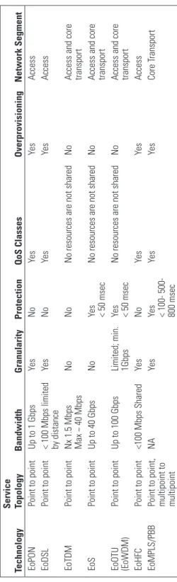
Table 3.17 summarizes the discussed technologies and their most impor-tant attributes. There is a clear separation for technologies into those that can be used in access segment and those that can be used in the core and handoff. In access, Ethernet may be provided over xPON, xDSL, fiber, TDM, HFC, SONET/SDH, and of course EoF. Technologies in access differ significantly by the granularity and limitation of the bandwidth available. Most of the ac-cess technologies are point to point. Some of them support CoS classes, some provide only one class of service, and some would allow overprovisioning. In the core and the handoff segments, Ethernet may be provided over SONET/ SDH, OTU, and fiber. These technologies scale up to over 10 GiGe, allow-ing different levels of aggregation and multiplexallow-ing. These technologies usually provide the protection (node and network) support < 100 ms restoration times. The transport technologies such as SONET/SDH and OTU may be enhanced by providing the packet awareness on the edges of the service or in the inter-mediate points. MPLS or PBB technologies add layer 2 features enhancing the service. However, they do require transport technologies underneath.

Figure 3.18 depicts the several modes of delivery of Ethernet services; the options are not exhaustive. As we indicated we have excluded wireless access,

(23)

Table 3.17

Ethernet Delivery T

echnologies and Their Support for Key Ethernet Service Features

Technology Service Topology Bandwidth Granularity Protection QoS Classes Overprovisioning Network Segment EoPON Point to point Up to 1 Gbps Ye s N o Yes Ye s Access EoDSL Point to point < 100 Mbps limited by distance Ye s N o Yes Ye s Access EoTDM Point to point Nx 1.5 Mbps Max ~ 40 Mbps No No

No resources are not shared

No

Access and core transport

EoS Point to point Up to 40 Gbps No Ye s < 50 msec

No

EoOTU (EoWDM) Point to point Up to 100 Gbps Limited; min. 1Gbps Ye s < 50 msec

No

EoHFC Point to point <100 Mbps Shared Ye s N o Yes Ye s Access EoMPLS/PBB

Point to point, multipoint to multipoint

NA Ye s Yes < 100- 500- 800 msec Ye s Yes Core T ransport

(24)

which may in some circumstances provide a valid transport technology option (in the access segment of the service in particular). MPLS may be extended over to the access and handoff segments. The core transport may include more complex combinations of layers such as Ethernet over pseudowires [42], over MPLS, over Ethernet and over OTU. Does this matter? It does, as each tech-nology has its limitations or advantages (i.e., certain technologies do not sup-port some service attributes or supsup-port them only in a limited way. Knowing the context of the MEBH service will tell us more about the ability of MEBH service to support the service requirements than any other information. In ad-dition, the overall Ethernet service properties are the result of the properties of the networking environment in which the Ethernet service is delivered. It is dif-ficult to predict exactly how the properties of specific technologies underlying the service will affect the overall service. It is difficult, but it does not mean that it can, or should, be ignored.

3.3 Service

Protection

3.3.1 Terminology

We begin with discussing the key concepts [43] describing resiliency and pro-tection design and service. The terms are not standardized and may be used and Figure 3.18 Ethernet delivery technologies data path.

(25)

interpreted in different ways. Thus, further discussion is beneficial to agree on what they mean.

3.3.1.1 Path

A path is a sequence of connected nodes and links with designated ingress and egress UNI and is capable of transferring traffic between ingress and egress CEs. Working path is the path used to forward service frames. Primary path is the preferred path for forwarding service frames between two or more UNIs. Backup path is a path that exists to carry service frames only if a failover event occurs on a primary path. Standby backup path is a backup path that is es-tablished prior to a failover event to protect a primary path. When a failover event is controlled by the customer, then the standby backup path will be a pre-established EVC.

3.3.1.2 Disjoint Path

For a service provider it means a pair of paths that do not share a common trans-port resources, such as links and nodes, other than ingress and egress UNIs. For a customer it means a pair of paths that do not share a common UNI.

3.3.1.3 Facilities

This is a physical resource in the transport network, such as a node, link, or path.

3.3.1.4 Protection

This is the architectural feature of a transport network that provides failure detection and failover from a primary service path to a backup service path or standby node when a failover event occurs. Protection switching is an action that redirects the traffic away from a working primary service path to a backup service path or standby node when a failover event occurs (e.g., a layer 2 switch-ing deployed as the protection method). Protection method is a mechanism that performs protection switching. Protection architecture is a transport network ar-chitecture that provides link, node, path protection, and/or other facilities upon a failover event on a primary service path. Reliability is a somewhat similar term defined as the ability of the system to operate uninterrupted (i.e., survive failures) [44].

3.3.1.5 Resiliency

This is a qualitative description of the capacity of a transport network to with-stand or recover from failed or degraded transport paths and facilities.

(26)

3.3.1.6 Redundancy

This is an architectural feature of a transport network that provides diverse facilities, such as standby nodes or standby paths over some or all of a primary service path.

3.3.1.7 Recovery

This is the action taken after a failover event whereby a node, link, or path is reinstated to its original state of performance.

3.3.1.8 Restoration

This is a state in which the primary service path has recovered from a failover event, but is not forwarding packets because the backup path remains the work-ing path.

3.3.1.9 Reversion

This is the state of failover recovery in which the primary service path has be-come the working path so that it is forwarding packets. Protection switching may or may not support reversion. If supported, must occur after restoration.

3.3.1.10 Domain

This is a group of arbitrarily connected transport facilities, possibly with some common characteristics (same administration, same technology, same risk).

3.3.1.11 (Shared) Risk Domain

This is a group of transport facilities, which could be a node, a link, a building, or the combination of any of these sharing the same risk.

3.3.1.12 Shared Risk Group (SRG)

SRG is a set of facilities sharing a common physical resource, including links and nodes (i.e., sharing a common risk). SRG is a composite of SRLG, SRNG, SRDG [45]. Shared risk link group is a group of links sharing the same risk do-main. Shared risk node group is a group of nodes sharing the same risk dodo-main. Shared risk domain group is a group of transport facilities sharing the same risk domain.

3.3.1.13 Diversity

Diversity is the architectural feature of a transport network that supports dis-joint shared risk groups (SRG) facilities for a primary service path. The concept of shared risk domains is illustrated in Figure 3.19 [46].

As an example we can differentiate several SRGs on the diagram. UNI-1, UNI-2, and UNI-3 are in SRNG with node NUNI-1, as the failure of the node N1 would interrupt the service to these UNIs. Node N1, link L1, and node

(27)

N2 are in the SRDG, as they are placed in the same location and are subject to possibly the same fault conditions (e.g., flood or power outage). All services going through the link L2 (from UNI-4 and UNI-5) are in the same SRLG, as they share the same link, and the failure of this link would affect these services. Other SRGs in Figure 3.19 can also be identified.

3.3.2 Concepts

In the nutshell, the protected network must have extra facilities that can be counted on supporting service if some part of the network fails. The most el-ementary protection design is a linear protection schema protecting a link be-tween two elements, in which two elements are connected over with two sepa-rate physical facilities, one of them active, another a stand-by service to protect the active one, as illustrated in Figure 3.20. In a case of failure, the traffic is switched from the active to standby.

In essence, the linear protection illustrates the generic concept of any pro-tected service. In any variant of the propro-tected design, the service has to have working and stand-by facilities, the failure detection mechanism responsible for detecting the failure of the working facility, and the switching mechanism that would switch the traffic between the working and stand-by facilities. Of course, in the real design we have complex protection configurations such as node protection, facilities protection, and virtualized facilities. Yet, it will not be an exaggeration to say that all of protected designs in essence resemble at some level of abstraction the protection configuration in Figure 3.20.

The resiliency of the network services and MEBH is a multilayer process. As we have mentioned in the previous sections, the Ethernet service is a layered Figure 3.19 Exemplar shared risk domains.

(28)

service. Always. Even in the simplest case of the native Ethernet transport, the Ethernet layer is riding over a layer 1 (i.e., the physical layer). It is because, every network service is in its essence a physical phenomenon. Thus, the resiliency of the Ethernet service is also a layered concept. This means that the resiliency of the Ethernet service is dependent on the resiliency of the layers below it. And, obviously, the resiliency of the layers above the Ethernet layer (that carry the services) depends on the resiliency of the Ethernet layer and all the layers below. Higher layers cannot recover before lower layers recover. Thus, the total recovery time of a given layer is a sum of recovery times of lower layers. As well, each layer has so called timeout or hold-off time. The timeout is a time interval a services at the given layer can survive the lack of connectivity. For the service to be resilient or protected, its hold-off time should be longer than the recovery times of layers below them. Or, the recovery times of lower layers should be shorter (in sum) than the time-outs of the services on the layers above. If the lower layers have longer recovery times than time-outs of the layers above, the services at the higher layers cannot be protected. This concept is presented in Figure 3.21.

The layer recovery times (Ti) add up to the total recovery time. If, as on

the diagram (B) of Figure 3.21 the hold-off time of the service at the layer x+1 is longer than the sum of recovery times of lower layers, then the service is protected. If, on the other hand, as on the diagram (A) the hold-off time of the service at the layer x+1 is shorter than the sum of recovery times of lower layers, then the service is not protected.

It is usual to compare any recovery times (of layers below layer 3) to the recovery time of SONET/SDH technology, which is around 50 milliseconds. Technologies of higher layers usually have longer recovery times—in a range of several hundred milliseconds to several seconds.

Some insights into the recovery process will foster better understanding of the protection processes. The recovery process is a series of events with time intervals between each event. Thus, the overall recovery time of the service is Figure 3.20 Link protection.

(29)

a sum of the component times of the recovery events. The recovery process is defined by the following events:

• Impairment event (Ie); • Fault detection event (Fde); • Hold-off event (Hoe);

• Connectivity restoration event (CRe); • Service restoration event (Sre).

At some point in time (T) the network element or service fails (Ie)—this is termed an impairment event and the time of the event is Tie. The event is detected—this is termed a fault detection event (Fde). The time of this event is TFde. The control plane waits for certain time before the recovery process is ini-tiated—this is called a hold-off event (Hoe). The hold-off event is terminated at time THoe. The recovery is completed and the connectivity is restored, which is a connectivity restoration event (CRe). This event happened at TCRe. After the connectivity is restored, the service may be restored, which is called service restoration event (SRe) at time TSRe [47]. Thus, the overall recovery time from failure to service recovery is the sum of all times listed above., and, one would add, at all layers carrying the service. This process is illustrated at Figure 3.22.

With some generalization, one may say that at every protocol layer the sequence of restoration events is similar.

(30)

Why it is important to recognize multievent, multilayered nature of the restoration process? It helps the provider and the customer to understand the impact of particular elements of the restoration process on the service and fine-tune the design. What counts for the customer is not necessarily the restoration of the connectivity at the lower layers but the restoration of his service. Even if the connectivity between the elements providing the service can be restored quite quickly (TCRe), the service itself (TSRe) may take a long time to be up again.

In some architecture, even if the connectivity at the transport layers (usu-ally layer 1 or 2) may be restored under several hundred milliseconds, the res-toration of the service (at layers 2+) may take 10 or more minutes [48] if the service has been lost. Imagine losing wireless service over a large geographical area for this period of time during rush hour. It certainly looks bad for the wire-less service. Thus, it may be the case that fine-tuning the fault detection and hold-over timers at the transport layers may save the provider long minutes of service blackouts, not to mention the poor PR and lost customers! How it is done? If the transport (or in general lower layers) can restore the layer-specific services within the hold-off time of the higher service layers, these layers may not declare the fault event and return to the service without interruption (i.e. without going into the full, long restoration process).

The protection design may be covering the UNI-to-UNI segment of the network, the UNI only, or any subsegment of the service. The better service protection is: less failures will affect the service and the service will recover in the shorter amount of time. To say it differently, protected service has high up time or availability.

Availability [49] of the service is expressed in the number of nines. Car-rier grade networks are generally targeted to provide five nines (or higher) Figure 3.22 Restoration events and timing.

THoe

TCRe

(31)

availability. Five nines means that out of some period of time, usually one year, the facility will be operation 99.999 percent of time. Table 3.18 provides the number of nines and the expected down time in a year, month, and week. One needs to understand that the number of nines expresses the long-term average behavior, not necessarily observable during a single reference period.

3.3.3 Estimating Availability

Availability is an elusive number and notoriously difficult to determine precise-ly. You could calculate the availability of service based on past experience. But this approach will tell us what did happen, not necessarily what will happen. In network design we want to be able to predict the resiliency of the design, before it is implemented, and compare different designs with respect to their reliability. The following method does just this. But a word of caution: as with any attempts to guess the future, this one is condemned to be as reliable as reading tea leaves. Yet it is “sanctioned” by the engineering praxis and imparts to the engineering estimates some aura of rational process. Availability is an es-timate of the uptime. Five nines (0.99999) availability in a year means that the object with this availability will be functioning 0.99999 of a year, or, it will not be operational for five minutes in a year. This number can be associated with any element of the network. The networks can be at the level of abstraction presented as a construct of the parallel and serial objects connected together as in Figure 3.23.

Each object can be assigned its availability, interpreted as the probability of being in the operational state during the specific time. The overall end-to-end availability of such a construct may be estimated using a simple math as illustrated here.

Table 3.18

Availability Rating and Outage Times Availability (Percent) Downtime per Year Downtime per Month* Downtime per Week 90 percent (“one nine”) 36.5 days 72 hours 16.8 hours 99 percent (“two nines”) 3.65 days 7.20 hours 1.68 hours

99.5 percent 1.83 days 3.60 hours 50.4 minutes

99.8 percent 17.52 hours 86.23 minutes 20.16 minutes 99.9 percent (“three nines”) 8.76 hours 43.2 minutes 10.1 minutes 99.95 percent 4.38 hours 21.56 minutes 5.04 minutes 99.99 percent (“four nines”) 52.56 minutes 4.32 minutes 1.01 minutes 99.999 percent (“fi ve nines”) 5.26 minutes 25.9 seconds 6.05 seconds 99.9999 percent (“six nines”) 31.5 seconds 2.59 seconds 0.605 seconds * 30 days per month

(32)

The objects A and B are connected together in series. Each object has availability of 0.9999. The availability of objects in series is estimated by the following formula:

A =Π A_i

where A_i is the availability of the i parallel component. Thus, the availability of the A and B object is

A = 0.9999 * 0.9999 = 0.9998

The objects C, D, and E are connected together in parallel. Each object has availability of 0.99. The availability of objects in parallel is estimated by the following formula:

A = 1 − π[1− Ai]

where Ai is the availability of the i component.

Thus, the availability of the objects C, D and E is

A = 1 − [1 − 0.99] * [1 − 0.99] * [1 − 0.99] = 0.999999

Thus, the summary availability of components can be substituted for the individual components; as a result, we have the series of components in series and the resultant availability is

A = 0.9998 * 0.999999 * 0.9999 = 0.99969

In principle every network can be reduced to such a calculation. Of course, the biggest problem is now how to interpret such a number in terms of the actual network behavior.

(33)

Availability [50] if not derived from the theoretical calculations [51] is estimated based on the past history of events. Two concepts are used here—that of mean time between failures (MTBF) and mean time to repair (MTTR). MTBF is the time the system or service has been operational [52]. MTTR is the average time it takes for the system or service to recover from failure. Avail-ability for the specific system or service is calculated in the following way:

A = MTBF/(MTBF + MTTR) × 100

In essence, the formula expresses the ratio of up time to total time elapsed. As with all statistical measures, this one is not the measure observable in a limited number of instances. It is an expected value over the long observation period. Thus, from time to time the highly reliable services and networks may fail (and they do) but do not lose their availability rating in the long run [53].

3.3.4 Protected Service Architectures

Many variants of network architecture can assure the reliability of the service. In general, the reliable service requires a resilient network. But it is not always the case. The highly resilient service may be implemented on the less resilient net-work. It means that the service with, for example, the five nines availability can be implemented on the network with the four nines availability rating. Follow-ing are some examples of resilient designs offerFollow-ing different levels of protection.

Figure 3.24 presents a design where the EVC has a unprotected handoff and an unprotected access facilities. The only protection offered here is the in-herent protection offered by the MEN network. In other words, the resiliency of this design relies on the availability of the MEN network.

Table 3.19 summarizes the resiliency features of this design.

Figure 3.25 illustrates the protected handoff design. This design uses a single EVC but two handoff points. Only one handoff point is active at the

(34)

time. The other is used as a backup facility. Table 3.20 summarized features of this design.

Figure 3.26 illustrates a design that uses two EVCs and two handoff points. Thus, in principle the transport and handoff points are protected through inde-pendent paths. Of course, for this schema to work the two EVCs should not be in the same SRG facilities. Table 3.21 details the resiliency of this design.

Figure 3.27 presents the protected access, transport, and handoff seg-ments. The service between the UNIs has two paths to traverse—one is active, and one is stand by. This is of course the most expensive protection mechanism. Table 3.22 details the resiliency of this design.

Figure 3.28 presents the variant of the design from Figure 3.27, where the protection facilities are provided by another carrier. Quite often this type of the design is used by customers demanding the ultimate failure resiliency. A design like this not only has to have independent dual paths, but it also has

Table 3.19

Failure Analysis—Single EVC Design Network

Segment Protection Failure Impact Access No protection in an access

segment.

Access to the CPE at UNI affected; service interrupted.

Transport Protection based on the MEN network design.

End-to-end service interrupted. If the MEN offers resiliency, the service may recover depending on the MEN resiliency design. The restoration time of several hundreds of milliseconds should suffi ce for most services with the exception of highly sensitive applications (e.g., emulated T1 (CES) pseudo wires). Handoff No protection in a handoff

segment.

Handoff affected all EVCs at this UNI. End to end EVC is protected only from the

failures in the MEN transport to the extent that the MEN network implements the resilient design.

Service is vulnerable to failures at handoff and access UNIs. MEN design may protect the service from transport failures. Such designs have usually less than four nines resiliency rating.

(35)

two different networks, assuming their independence, isolating events in one network from operations of the other one.

Of course, one may have dual access protection without the protection of the transport and handoff. Or, one may protect the access facilities but not handoff or transport. One may also protect part of the transport only. Thus, the possible combinations of protection design are many, and what is presented here are canonical cases only. The decision how to implement the protection design as it was discussed depends on which part of the network supporting the service is the most critical one to the service overall continuity [54].

Figure 3.26 Two EVCs with two handoffs. Table 3.20 Dual Handoff Architecture Network

segment

Transport Protection based on the MEN network design

End-to-end service interrupted. If the MEN offers resiliency, the service may recover depending on the MEN resiliency design. The restoration time of several hundreds of milliseconds should suffi ce for most services with the exception of highly sensitive applications (e.g., emulated T1 (CES) pseudo wires). Handoff Dual handoff to the customer

premises

If handoff fails, the service should switch to the standby handoff interface and the service should recover within the specifi ed interrupt time The restoration time of several hundreds of milliseconds should suffi ce for most services with the exception of highly sensitive applications (e.g., emulated T1 (CES) pseudo wires).

End to end EVC is protected from the failures in the MEN transport by the network protection mechanism and at the handoff by the dual handoff.

The overall service resiliency is improved as part of the service has parallel facilities. Such designs have usually around four nines resiliency rating with the resiliency of the handoff above four nines.

(36)

3.3.5 Implementation

The protection is expensive: it requires redundant facilities. Thus, in building protection in the network, one must exercise the sound judgment to strike a balance between redundancy, a required level of protection, and expected avail-ability. One way to evaluate the effect of the protection design is to calculate the hypothetical cost of offering the protection to the number of megabits per second protected. For example, if the protection is built to protect the UNI interface with a 100-Mbps interface, the cost of the protection mechanism will be allocated to the UNI bandwidth of 100 Mbps. If the protection mechanism is built to protect a 10,000-Mbps UNI, the cost will be allocated to 10,000 Figure 3.27 Two EVCs with dual access, dual handoff, and protected transport.

Table 3.21

Two EVCS and Two Handoff Design Network

segment.

Transport Protection is achieved by dual transport paths—one active, one stand by.

End-to-end service interrupted. If the MEN offers resiliency, the service may recover depending on the MEN resiliency design The restoration time of several hundreds of milliseconds should suffi ce for most services with the exception of highly sensitive applications (e.g., emulated T1 (CES) pseudo wires). Handoff Dual handoff to the customer

premises.

If handoff fails, the service should switch to the stand-by handoff interface, and the service should recover within the specifi ed interrupt time. The restoration time of several hundreds of milliseconds should suffi ce for most services with the exception of highly sensitive applications (e.g., emulated T1 (CES) pseudo wires).

End to end EVC is protected from the failures in the MEN transport and at the handoff by the dual handoff.

The service protection is improved considerably as the service has two parallel paths that are not in the same SRG (this is the assumption). The service should be protected from the failure in transport and handoff segments. Such designs have usually greater than four nines resiliency rating.

(37)

Mbps. Thus, protecting access interfaces is expensive and rarely done. But the protection of the aggregated handoff interfaces is less expensive per bit, and

Table 3.22

Two EVCs with Dual Access, Transport, and Handoff Facilities Network

Segment Protection Failure Impact

Access Dual access. Access to the CPE at UNI protected by the dual access facilities. If the stand-by and active paths do are not in SRG facilities, then the failure of one path should not affect the service. The restoration time of several hundreds of milliseconds should suffi ce for most services with the exception of highly sensitive applications (e.g., emulated T1 (CES) pseudo wires). Transport Protection is achieved by dual

transport paths—one active, one stand by.

If the stand-by and active paths do are not in SRG facilities, then the failure of one path should not affect the service. The restoration time of several hundreds of milliseconds should suffi ce for most services with the exception of highly sensitive applications (e.g., emulated T1 (CES) pseudo wires). Handoff Dual handoff to the customer

premises.

If handoff fails, the service should switch to the stand-by handoff interface and the service should recover within the specifi ed interrupt time. The restoration time of several hundreds of milliseconds should suffi ce for most services with the exception of highly sensitive applications (e.g., emulated T1 (CES) pseudo wires).

End to end EVC is protected from the failures in the MEN transport and at the handoff by the dual handoff.

The service is protected by two parallel paths, earning the high protection rating. Such systems may achieve fi ve nines or six nines resiliency rating.

(38)

that is why it is more frequently deployed. Other ways to evaluate the effective-ness of the protection is to compare number of EVCs projected or a number of UNIs protected. Of course, there is a common-sense interpretation of these metrics as well: it makes more sense to invest into the protection of facilities with many services riding on them rather than the protection of facilities with a small amount of services. This concept is illustrated in Figure 3.29. Protect-ing individual UNIs with a sProtect-ingle EVC and 100-Mbps bandwidth is much less cost effective than protecting a handoff UNI with many EVCS and 10 Gbps of combined traffic. The hypothetical protection curve for Mbps and EVCs is provided in Figure 3.30.

3.3.6 Measuring Resiliency

Resiliency of every property of the service of network can be measured. Apart from the availability, other metrics can be used to characterize the operational characteristics of the network. The metrics [55] for this purpose are not widely used, but their understanding would be beneficial for the customer, as these metrics characterize (and provide insights into) the network protection design and its impact on the service. Of course, the metrics listed here are not an ex-haustive list of metrics available for this purpose.

3.3.6.1 Failover Packet Loss

This is the amount of packet loss produced by a failover event until the failover completes, where the measurement begins when the last unimpaired packet is

(39)

received by the tester on the protected primary path and ends when the first unimpaired packet is received by the tester on the backup path.

3.3.6.2 Reversion Packet Loss

This is the amount of packet loss produced by reversion, where the measure-ment begins when the last unimpaired packet is received by the tester on the backup path and ends when the first unimpaired packet is received by the tester on the protected primary path .

3.3.6.3 Failover time

This is the amount of time it takes for the failover to complete so the backup path is established as a working path.

3.3.6.4 Reversion Time

This is the amount of time it takes for reversion to complete so that the primary path is restored as the working path.

3.3.6.5 Additive Backup Delay

This is the amount of increased forwarding delay resulting from data traffic traversing the backup path instead of the primary path. Additive backup delay is calculated using the formula shown here:

(

)

(

)

Additive Backup Delay Forwarding Delay Forwarding Delay Backup Path Primary Path

= −

(40)

While these metrics maybe difficult to measure in real services, one may use these concepts to quantify the properties of the network. For example, one may establish as part of the service specification a maximum failover time and reversion time required for the service on failure event. One may also explicitly request that the additive backup delay is bound by the same limits as a delay time on the primary path.

3.4 Quality of Service

The quality of service (QoS) mechanisms are designed to manage transport of service frames through the network assuring some level of consistency in treat-ing of packets in case of congestion (observe that fully provisioned networks such as SONET do not have similar QoS mechanisms, as they do not need to resolve congestion conditions). Depending on the class of service (CoS) as-signed to service frames, these mechanisms may pass certain frames ahead of others, delay some of them, or drop them. In general QoS mechanisms enforce service parameters grouped under the concept of QoS service classes. Service frames with a so called high QoS class get better performance characteristics than do frames with lower CoS classes. The specific CoS class of a frame may be signaled in the network using the PCP field in the Ethernet VLAN tag (in-band signaling) or imposed by the out-of-band provisioning. The QoS characteristics of the service are organized into the QoS profiles or QoS policies. The QoS profile includes bandwidth parameters and flow performance characteristics per class of traffic. The following sections describe elements that constitute the QoS profiles as well as mechanisms that enforce QoS policies [56].

3.4.1 Bandwidth Concepts

The bandwidth or transmission rate is the number of traffic units (bits, bytes, octets, frames, or packets) per second transmitted over the interface. The trans-mission rate may be expressed in bits per second, frames or packets per second, or octets per second. Depending on which transmitted bits are counted toward the rate, we can define protocol transmission rate (counting bits of the specific protocol only), physical transmission rate (counting all the bits passing through the interface), or service transmission rate (counting only the bits that are part of the service). Bits per second can be used to characterize both physical media and services. Frames are most often used to characterize services. The frame used to characterize the transmission rate may include all or some aspects of the protocol the service frame belongs to. In the Ethernet services we define the concept of the service frame. The service frame includes all the fields in the Ethernet II frame from the first bit of the MAC DA address field to the last bit of the FCS field, but it excludes the control fields PRE, SDF, and IFG. The

(41)

control fields are referred to as Ethernet protocol overhead. For the same bit rate, one will get different frame rates depending on whether one counts frames with or without the overhead.

Frames are transmitted with certain rate of frames per second. The maxi-mum long-term average rate of transmission for which the delivery of frames is guaranteed is called committed information rate (CIR) and is characterized by bits per second. CIR approximates the transmission in which frames are sent with relatively equal interframe intervals as illustrated in Figure 3.31.

Figure 3.31 illustrates the transmission rate of 8 frames per second (fps) of 100 bits per frame, or 800 bits per second, or 100 octets per second. The same rate of transmission may be achieved when the frames are transmitted over shorter than 1-second time frames followed by the periods of no transmission, as illustrated in Figure 3.32.

In this case, all frames are transmitted in a fraction of a second followed by the period of no transmission. Such a transmission is called bursting (op-posed to the uniform transmission from the previous example) or back-to-back transmission. The parameter that defines the ability of the interface to transmit burst of traffic is called committed burst size (CBS). CBS is measured in bytes.

3.4.2 Bandwidth Enforcement 3.4.2.1 Policing

The bandwidth is defined by CIR, CBS, EIR, and EBS parameters. We have explained already CIR as a long-term average guaranteed bit rate and CBS as a number of bytes that can be transported back to back without violating CIR. The excess information rate (EIR) and the corresponding excess burst size (EBS)

Figure 3.31 Transport of service frames at regular intervals.