Fully Implicit Time Stepping Can Be Efficient on Parallel Computers

Fully Implicit Time Stepping Can Be Efficient on Parallel

Computers

Brandon Cloutier1_{, Benson K. Muite}2_{, Matteo Parsani}3

c

The Authors 2019. This paper is published with open access at SuperFrI.org

Benchmarks in high performance computing often involve a single component used in the full solution of a computational problem, such as the solution of a linear system of equations. In many cases, the choice of algorithm, which can determine the components used, is also important when solving a full problem. Numerical evidence suggests that for the Taylor–Green vortex problem at a Reynolds number of 1600, a second order implicit midpoint rule method can require less computational time than the often used linearly implicit Carpenter–Kennedy method for solving the equations of incompressible fluid dynamics for moderate levels of accuracy at the beginning of the flow evolution. The primary reason is that even though the implicit midpoint rule is fully implicit, it can use a small number of iterations per time step, and thus require less computational work per time step than the Carpenter–Kennedy method. For the same number of timesteps, the Carpenter–Kennedy method is more accurate since it uses a higher order timestepping method.

Keywords: incompressible Navier–Stokes equations, parallel computing, spectral methods, time stepping.

Introduction

Benchmarks in parallel computing are often micro-benchmarks or computationally expensive components of full applications, such as solvers for linear systems. It is often the case that the choice of numerical method can be as important as the optimization of the component subroutines. To be able to compare different choices of numerical methods, full application benchmarks are also very useful. The International Workshops on High Order Computational Fluid Dynamics methods [7, 12] are a conference series with the aim of comparing the speed and accuracy of computational fluid dynamics software for solving particular well defined problems. One of the considered cases is the Taylor–Green vortex at a Reynolds number of 1600. This is a case where there is a vortex instability which is difficult to compute correctly using low resolution or a poor numerical method [24]. While there are a wide range of spatial discretization methods suitable for solving the Navier–Stokes equations, Fourier spectral methods are a class of methods where the choice of time stepping procedure on the effectiveness of solving a partial differential equation can be easily investigated [20]. By comparing two different time stepping regimes, one can also determine whether discretization methods which have conserved discrete analogues of the continuum conserved quantities are well suited for approximating turbulent flows, and will be useful in engineering applications where time and cost to solution are important.

Following this introduction, Section 1 introduces the incompressible Navier–Stokes equa-tions; the numerical algorithms which use the Fast Fourier transform as a component are de-scribed in the Section 2. A description of the massively parallel computational platform used is in Section 3. The results of the computational experiments are described in Section 4. This is then followed by the conclusion.

1_{University of Michigan, Ann Arbor, Michigan, USA} 2_{Tartu ¨Ulikool, Tartu, Estonia}

1. Incompressible Navier–Stokes Equations

The incompressible Navier–Stokes equations written in dimensionless form are:

∂u

∂t +u· ∇u=−∇ ·p+

1

Re∆u, ∇ ·u= 0, (1)

where u ∈ _R3 _{is the velocity vector and p ∈}

R is the pressure. Here Re denotes the Reynolds

number that characterizes the flow and it is defined as

Re = ρref|uref|Lref

µref

, (2)

where ρref, |uref|, Lref, µref and are the (constant) density of the fluid, the modulus of a

representative velocity, a characteristic length and the dynamic viscosity, respectively.

2. The Numerical Method

A Fourier spectral method is used to perform a direct numerical simulation of the Taylor– Green vortex for the incompressible Navier–Stokes equations. For the Taylor–Green vortex flow, given the periodic square box [−mπ, mπ]3 (which defines the computational domain) and the initial velocity field, the representative length scale and velocity module are set equal to the mul-tiplem of the “standard” box width 2π (i.e.,Lref =m) and the maximum velocity component

of the initial flow field.

The parallel codes are available at [9, 10]. They use MPI and are similar to the example programs available at [4]. The library 2DECOMP&FFT is used for the domain decomposition and the parallel fast Fourier transforms [21].

In both implicit midpoint rule (IMR) and Carpenter–Kennedy [5] (CK) time stepping schemes, the time advancement is done in Fourier space and the nonlinear terms are calcu-lated by transforming to real space, multiplying and then transforming back to Fourier space. Following [6], we do not de-alias our schemes because the simulations are fully resolved. Visual-ization is done using Octave [15], Matlab, Python (Matplotlib [19]), Paraview [2] and VisIt [8].

2.1. Implicit Midpoint Rule

The implicit midpoint rule is

un+1,j+1−un

δt +

un+1,j+un

2 · ∇

un+1,j+un

2

= ∇

∆−1 ∇ ·

(un+1,j+un)· ∇(un+1,j+un)

4 + ∆

un+1,j+1+un

2Re , (3)

where j is the iterate andn is the timestep. Note that the implementation of the IMR in this study uses fixed point iteration with the stopping critera that the change between successive iterations is less than 10−10_{in the sum of thel}∞ _{norms of the components of the individual flow} field components. The method requires three levels of storage for un+1,j+1_,un+1,j _{and u}n_{, and}

uses 15 Fast Fourier Transforms per iteration.

The IMR method also has discrete analogues for energy and enstrophy dissipation:

1 2

Z

Ω

d(u·u)

dt =−

1

Re

Z

Ω

Z

Ω

un+1·un+1−un·un

2δt =−

1 4Re

Z

Ω

∇ un+1+un· ∇ un+1+un, (5)

1 2

Z

Ω

d(ω·ω)

dt =−

1

Re

Z

Ω

∇ω· ∇ω, (6)

Z

Ω

ωn+1·ωn+1−ωn·ωn

2δt =−

1 4Re

Z

Ω

∇ ωn+1+ωn

· ∇ ωn+1+ωn

. (7)

2.2. Carpenter–Kennedy Method

The CK method consists of splitting the equation into linear and nonlinear parts,

l(u) = 1

Re∆u, (8)

g(u) =−u· ∇u+∇

∆−1(∇ ·[u· ∇u]) (9)

and then solving the linear part implicitly, and the nonlinear part explicitly, using the steps detailed in Algorithm 1, where in line 5

α= [0.0,0.1496590219993,0.3704009573644,0.6222557631345,0.9582821306748,1.0],

β = [0.0,−0.4178904745,−1.192151694643,−1.697784692471,−1.514183444257]

and in line 6

γ = [0.1496590219993,0.3792103129999,0.8229550293869,0.6994504559488,0.1530572479681].

The algorithm requires two levels of storage h and u and uses 70 FFTs per timestep. Thus, if the IMR method requires 4 or fewer iterations per timestep, it can require less time to complete than the CK method.

Algorithm 1 The CK time stepping algorithm for the 3D incompressible Navier-Stokes

equa-tions

1: input un

2: u=un 3: h=0

4: for k= 1 to 5 do

5: h←g(u) +βkh µ←0.5δt(αk+1−αk)

6: Solve v−µl(v) =γkδth+µl(u) for v

7: u←v

8: end for

9: un+1 =u

3. Computational Platform

Numerical experiments have been performed on a variety of computational platforms, which are listed in the acknowledgements. The results reported here were obtained on Hazelhen [18] a Cray XC 40 supercomputer with dual IntelR _XeonR _{CPU E5-2680 v3 (30M Cache, 2.50 GHz)} processors per node. This supercomputer uses an Aries interconnect [17]. As this computer has a network where congestion effects can change runtime, reported results were run on 768 cores for which repeated short runs showed that the typical standard deviation in the runtime was 20% [3], see also Fig. 10. Access to a computer system with a network that isolates communication for a particular job to a particular subnetwork (such as found on supercomputers with torus networks) was not available for this study.

The source codes [9, 10] were compiled with GCC GNU Fortran compilers using the Cray provided wrappers (ftn) and optmization flag -O3. 2DECOMP&FFT [21] was used as the parallel Fourier transform and domain decomposition library, with FFTW 3.3.4.7 as the one dimensional Fast Fourier transform library.

4. Results

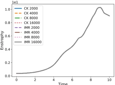
To ensure verifiability of the computed results, the benchmark case requires production of data for the kinetic energy (Fig. 1), kinetic energy dissipation rate (Fig. 2) and enstrophy (Fig. 3) evolution for the Taylor–Green Vortex between times of 0 and 10. Also required is a plot of the midplane vorticity (Fig. 4) at a time of 8, when the enstrophy and kinetic energy dissipation rates are at their peaks. Reference values for these are given by the organizers to allow for comparison with submitted solutions. Many previous submissions have typically reported solutions with 2-3 digits of accuracy. The programs and data to produce all figures except Fig. 4 are in [11].

0 2 4 6 8 10

Time

0.09 0.10 0.11 0.12

Kin

eti

c e

ne

rgy

CK 2000 CK 4000 CK 8000 CK 16000 IMR 2000 IMR 4000 IMR 8000 IMR 16000

0 2 4 6 8 10

Time

0.0 0.2 0.4 0.6 0.8 1.0 1.2

Kin

eti

c e

ne

rgy

di

ssi

pa

tio

n r

ate

1e−2

CK 2000 CK 4000 CK 8000 CK 16000 IMR 2000 IMR 4000 IMR 8000 IMR 16000

Figure 2. Kinetic energy dissipation rate. Legend indicates time stepping scheme and number

of timesteps

0 2 4 6 8 10

Time

0.2 0.4 0.6 0.8 1.0

En

str

op

hy

1e1

CK 2000 CK 4000 CK 8000 CK 16000 IMR 2000 IMR 4000 IMR 8000 IMR 16000

Figure 3. Enstrophy. Legend indicates time stepping scheme and number of timesteps

4.2. Comparison between the Implicit Midpoint Rule and Carpenter–Kennedy Methods

The IMR requires 15 fast Fourier transforms per iteration, while the CK method requires 70 iterations per timestep. Thus for a single timestep, if 4 or fewer iterations are needed, the IMR method will require less time to solution than the CK method. The IMR method is a second order method, while the CK method is a third order method, though for high Reynolds number flows, behaves like a fourth order method. Nevertheless, the IMR method should be good at capturing statistical behavior of turbulent flows.

−3 −2.5 −2 −1.5

−1 −0.5 0

5 10 15 20 25 30

Figure 4.Isocontours of the midplane vorticity at a time of 8, due to symmetry only a quarter

of the midplane is shown

0 2 4 6 8 10

Time

10 20 30 40 50 60

Ite

rat

ion

s

IMR 2000 IMR 4000 IMR 8000 IMR 16000

Figure 5. Iterations required for convergence to the required tolerance for the IMR scheme

during the temporal flow field evolution. Legend indicates the number of timesteps

Table 1.Performance on Hazelhen [18]. All computations are done from a time of 0

to a time of 10 on 768 cores for a 5123 discretization

Method Time steps Time(s) Core hours FFTs/Timestep

IMR 2000 10369 2212.1 254.8

CK 2000 2513 536.1 70

IMR 4000 8295 1769.6 112.7

CK 4000 5176 1104.2 70

IMR 8000 13199 2815.8 88.9

CK 8000 10722 2287.4 70

IMR 16000 21918 4675.8 72.45

0 2 4 6 8 10

Time

0 1 2 3 4

En

str

op

hy

1e−3

CK 2000 - IMR 16000 CK 4000 - IMR 16000 CK 8000 - IMR 16000 CK 16000 - IMR 16000 IMR 2000 - IMR 16000 IMR 4000 - IMR 16000 IMR 8000 - IMR 16000

Figure 6. Differences between the enstrophy computed with the IMR scheme using 16000

timesteps and CK and IMR schemes. Legend indicates the number of timesteps

0 2 4 6 8 10

Time

−1 0 1

En

str

op

hy

1e−6

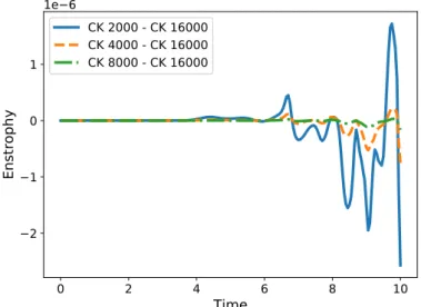
CK 2000 - CK 16000 CK 4000 - CK 16000 CK 8000 - CK 16000

Figure 7.Differences between the enstrophy computed with CK schemes. Legend indicates the

number of timesteps

Finally, Fig. 10 shows that for the first 20 timesteps of a 2000 timestep run, the IMR and CK methods have the same runtime.

Conclusions

0 2 4 6 8 10

Time

0 1 2 3 4 5

Kin

eti

c e

ne

rgy

di

ssi

pa

tio

n r

ate

1e−6

CK 2000 - IMR 16000 CK 4000 - IMR 16000 CK 8000 - IMR 16000 CK 16000 - IMR 16000 IMR 2000 - IMR 16000 IMR 4000 - IMR 16000 IMR 8000 - IMR 16000

Figure 8.Differences between the kinetic energy dissipation rates computed with the IMR and

CK schemes. Legend indicates the number of timesteps

0 2 4 6 8 10

Time

−2 −1 0 1 2

Kin

eti

c e

ne

rgy

di

ssi

pa

tio

n r

ate

1e−9

CK 2000 - CK 16000 CK 4000 - CK 16000 CK 8000 - CK 16000

Figure 9. Differences between the kinetic energy dissipation rates computed with the CK

method. Legend indicates the number of timesteps

transform, such as finite difference or finite element methods, to give moderate accuracy results with relatively low computation times.

Relying on classical schemes may be inappropriate, especially for computationally costly simulations where statistical reproducibility but not point wise accuracy is required. Thus in addition to semi-implicit schemes such as the Carpenter–Kennedy method, fully implicit schemes should also be considered as they may be computationally efficient [23]. This is because for time evolutionary schemes (as opposed to stationary problems as considered in other studies [1, 13, 22]), a good initial iterate obtained from the numerical approximation at the previous time step can make the number of iterations required for convergence of the iterative scheme small. In the atmospheric simulations [25] it has also been observed that implicit schemes may give a faster time to solution than explicit schemes, despite having lower scalability and a lower floating point efficiency.

102 ₁₀3 ₁₀4

Cores

Tim

e (

s)

CK IMR

Figure 10. Strong Scaling for the first 20 timesteps of a 2000 timestep run modified from [3].

Error bars represent maximum and minimum runtimes

is challenging to find studies that combine both domain specific and high performance com-puting knowledge. Domain specific community benchmarking efforts, such as the International Workshop on High Order Computational Fluid Dynamics serve as a very useful complement to traditional high performance computing benchmarks such as Linpack [14]. Such efforts will become much more relevant in the future as most scientific computing will necessarily be parallel.

Acknowledgements

We thank the reviewers for their constructive comments, and Koen Hillewaert and David Ketcheson for helpful advice. We thank the participants of the 2013 HiOCFD workshop [12] for feedback on an earlier version of this work that enabled greater examination of the numerical results. BKM thanks Arieh Iserles for pointing out the geometric properties of the implicit midpoint rule and Charles Doering, Jos´e Gracia, Hans Johnston, Ning Li, Peter Van Keken, Divakar Viswanath and Jared Whitehead for helpful discussion. BKM was partially supported by HPC Europa 3 (INFRAIA-2016-1-730897). The computational resources used to build and test the programs were:

• Flux operated at the University of Michigan.

• Keeneland initial delivery system operated by Georgia Tech and the National Institute for Computational Sciences.

• Noor operated by KAUST information technology services.

• Shaheen and Shaheen II operated by the KAUST Supercomputing Laboratory.

• Hazelhen and Kabuki at HLRS.

Flow field visualization was aided by an extended collaborative support allocation from the extreme digital science and discovery environment (XSEDE) which is supported by National Science Foundation grant number OCI-1053575. We thank Mark Vanmoer for help with this.

References

1. Adams, M.F., Brown, J., Shalf, J., Straalen, B.V., Strohmaier, E., Williams, S.: HPGMG 1.0: A benchmark for ranking high performance computing systems. Tech. Rep. LBNL 6630E, Lawrence Berkeley National Laboratory, Berkeley, California, USA (2014). https:

//escholarship.org/uc/item/00r9w79m, accessed: 2019-07-17

2. Ahrens, J., Geveci B., Law C.: ParaView: An End–User Tool for Large Data Visualization, In the Visualization Handbook. Edited by Hansen C.D. and Johnson C.R., Elsevier (2005).

http://www.paraview.org/, accessed: 2019-06-24

3. Aseeri, S., Muite, B.K., Takahashi, D.: Reproducibility in Benchmarking Parallel Fast Fourier Transform based Applications. In: Companion of the 2019 ACM/SPEC International Con-ference on Performance Engineering, ICPE ’19, 7-11 April 2019, Mumbai, India. pp. 5–8. ACM (2019), DOI: 10.1145/3302541.3313105

4. Balakrishnan, S., Bargash, A.H., Chen, G., Cloutier, B., Li, N., Malicke, D., Muite, B.K., Quell, M., Rigge, P., San Roman Alerigi, D., Solimani, M., Souza, A., Thiban, A.S., West, J., van Moer, M.: Parallel Spectral Numerical Methods. http://en.wikibooks.org/wiki/

Parallel_Spectral_Numerical_Methods, accessed: 2019-06-24

5. Carpenter, M.H., Kennedy, C.A.: Fourth–Order 2N–Storage Runge–Kutta schemes, NASA Langley Research Center Technical Memorandum 109112.https://ntrs.nasa.gov/search.

jsp?R=19940028444 (1994), accessed: 2019-07-17

6. Canuto, C., Hussaini, M.Y., Quarteroni, A., Zang, T.A.: Spectral methods fundamentals in single domains, Springer (2010), DOI: 10.1007/978-3-540-30726-6

7. Cenaero: Fifth International Workshop on High–Order CFD Methods. https://how5. cenaero.be/, accessed: 2019-06-24

8. Childs, H., Brugger, E., Bonnell, K., Meredith, J., Miller, M., Whitlock, B., Max, N.: A contract–based system for large data visualization, IEEE Visualization 2005, 190–198, (2005).

https://wci.llnl.gov/codes/visit/, accessed: 2019-06-24

9. Cloutier, B.: MPI Fortran Implicit Midpoint Rule Incompressible Navier–Stokes Solver. https://github.com/bcloutier/PSNM/blob/master/NavierStokes/Programs/

NavierStokes3dFortranMPI/navierstokes_IMR.f90, accessed: 2019-06-24

10. Cloutier, B.: MPI Fortran Carpenter-Kennedy Incompressible Navier–Stokes Solver. https://github.com/bcloutier/PSNM/blob/master/NavierStokes/Programs/

NavierStokes3dFortranMPI/navierstokes.f90, accessed: 2019-06-24

11. Cloutier, B., Muite, B.K., Parsani, M.: Fully Implicit Time Stepping can be Efficient on Parallel Computers [Data set], Zenodo, DOI: 10.5281/zenodo.2667709

12. Deutsches Zentrum f¨ur Luft- und Raumfahrt (DLR): Second International Workshop on High–Order CFD Methods. https://www.dlr.de/as/desktopdefault.aspx/tabid-8170/

13. Dongarra, J., Heroux, M., Luszczek, P.: HPCG benchmark: a new metric for ranking high performance computing systems. The International Journal of High Performance Computing Applications 30(1), 3–10 (2015), DOI: 10.1177/1094342015593158

14. Dongarra, J., Luszczek, P., Petitet, A.: The LINPACK benchmark: Past, present and future. Concurrency and Computation: Practice and Experience 38(9), 803–820 (2003), DOI: 10.1002/cpe.728

15. Eaton, J. W., Bateman, D., Hauberg, S., Wehbring, R.: GNU Octave version 4.2.1 man-ual: a high–level interactive language for numerical computations. https://www.gnu.org/

software/octave/doc/v4.2.1/ (2017), accessed: 2019-06-24

16. Elcott, S., Tong, Y., Kanso, E., Schr¨oder, P., Desbrun, M.: Stable, circulation– preserving, simplicial fluids. ACM Transactions on Graphics 26(1), 4 (2007), DOI: 10.1145/1189762.1189766

17. Faanes, G., Bataineh, A., Roweth, D., Court, T., Froese, E., Alverson, B., Johnson, T., Kopnick, J., Higgins, M., Reinhard, J.: Cray Cascade: A scalable HPC system based on a Dragonfly network. In: SC’12: Proceedings of the International Conference on High Perfor-mance Computing, Networking, Storage and Analysis, 1–9 (2012), DOI: 10.1109/SC.2012.39

18. H¨ochstleistungsrechenzentrum Stuttgart (HLRS): Hazelhen. https://www.hlrs.de/

systems/cray-xc40-hazel-hen/, accessed: 2019-06-24

19. Hunter, J.D.: Matplotlib: A 2D graphics environment. Computing in Science and Engineer-ing 9(3), 90–95 (2007), DOI: 10.1109/MCSE.2007.55

20. Ketcheson, D.I., Mortensen, M., Parsani, M., Schilling N.: More efficient time integration for Fourier pseudo–spectral DNS of incompressible turbulence, arXiv: 1810.10197v1, accessed: 2019-07-17

21. Li, N., Laizet, S.: 2DECOMP&FFT – A highly scalable 2D decomposition library and FFT interface, Cray User Group 2010, Edinburgh, UK. http://www.2decomp.org/pdf/

17B-CUG2010-paper-Ning_Li.pdf, accessed: 2019-07-17

22. M¨uller, E.H., Scheichl, R., Vainikko, E.: Petascale solvers for anisotropic PDEs in atmospheric modelling on GPU clusters. Parallel Computing 50, 53–69 (2015), DOI: 10.1016/j.parco.2015.10.007

23. Parsani, M., Van den Abeele, K., Lacor, C. and Turkel, E.: Implicit LU–SGS algorithm for high–order methods on unstructured grid with p–multigrid strategy for solving the steady Navier–Stokes equations. Journal of Computational Physics 229(3), 828–850 (2009), DOI: 10.1016/j.jcp.2009.10.014

24. van Rees, W.M., Leonard, A., Pullin, D.I., Koumoutsakos, P.: A comparison of vortex and pseudo–spectral methods for the simulation of periodic vortical flows at high Reynolds numbers. J. of Computational Physics 230, 2794–2805 (2011), DOI: 10.1016/j.jcp.2010.11.031