DYNAMIC PROGRAMMING APPROACH TO TESTING RESOURCE ALLOCATION PROBLEM FOR MODULAR SOFTWARE

DYNAMIC PROGRAMMING APPROACH

TO TESTING RESOURCE ALLOCATION

PROBLEM FOR MODULAR SOFTWARE

P.K. Kapur

1

P.C. Jha

1

A.K.

Bardhan

1

Abstract

Testing phase of a software begins with module testing. During this period modules are tested independently to remove maximum possible number of faults within a specified time limit or testing resource budget. This gives rise to some interesting optimization problems, which are discussed in this paper. Two Optimization models are proposed for optimal allocation of testing resources among the modules of a Software. In the first model, we maximize the total fault removal, subject to budgetary Constraint. In the second model, additional constraint representing aspiration level for fault removals for each module of the software is added. These models are solved using dynamic programming technique. The methods have been illustrated through numerical examples.

Key words:Software Reliability, Non Homogeneous Poisson Process, Resource Allocation, Dynamic Programming

1. Introduction

Growth in software engineering technology has led to production of software for highly complex situations occurring in industry, scientific research, defense and day to day life. Consequently, the dependence of mankind on computers and computer-based systems is increasing day by day. Any failure in these systems can cost heavily in terms of money and/or human lives. Though high reliability of hardware part of these systems can be guaranteed, the same cannot be said for software. Therefore a lot of importance is attached to the testing phase of the software development process, where around half the developmental resources are used [8]. Essentially testing is a process of executing a program with the explicit intention of finding faults and it is this phase, which is amendable to mathematical modeling. It is always desirable to remove a substantial number of faults from the software. In fact the reliability of a software is directly proportional to the number of faults removed. Hence the problem of maximization of software reliability is identical to

1

that of maximization of fault removal. At the same time testing resource are not unlimited, and they need to be judiciously used. In this paper we discuss and solve such a management problem of allocation of testing resources among modules, through a Software Reliability Growth Model (SRGM). A Software Reliability Growth Model (SRGM) is a relationship between the number of faults removed from a software and the execution time/CPU time/calendar time. Several attempts have been made to represent the actual testing environment through SRGMs [1,4,5,9]. These models have been used to predict the fault content, reliability and release time of a software. SRGMs have also been used to manage the testing phase. Again large software consists of modules. Often these modules are developed independently and each module may contain different number of faults and that of different severity. Therefore distinct SRGMs should be used to represent the testing process of each module, as testing for these modules are done independently. An SRGM with testing effort [9] has been chosen to represent the fault removal process for the two optimization problems discussed in this paper.

The first optimization model (P1) maximizes the total number of faults expected to be removed, when available testing resource is known. The management normally aspires for some reliability level that can be translated in terms of number of faults removed. In the second optimization model (P2) we add a constraint in (P1) in terms of minimum number of faults aspired to be removed from each module. Dynamic programming technique is used to solve these problems. This is the first time that this has been done in software engineering, according to our knowledge. Dynamic programming approach, which is easy to solve and understand provides global optima for these problems. The methodology discussed in the paper has been illustrated through numerical examples.

Notations

N : Number of modules in the Software (>1)

ai : Expected number of faults in the ith module (i=1,2,…,N) bi : Proportionality constant for the ith module

xi(t) : Current testing effort expenditure at testing time t

and

=

∫

t i i

t

x

w

dw

X

0

)

(

)

(

for ith module

Xi, Z : The amount of testing resource to be allocated to the i

th

module and total testing resource available.

mi(t) : Number of faults removed in (0,t] the ith module,

mean value function of NHPP, i = 1,…,N T : Total testing time

Xi* : Optimal value of Xi , i = 1,…,N

fn(Z) : Optimal number of faults removed upto nth modules (i.e.

aio : Aspiration level of ith module (i.e. number of faults desired to be

removed from ith module)

pi : The minimum proportion of total faults to be removed from

ith module.

2. Mathematical

Modelling

2.1 Resource Allocation Problem

Consider a software having N modules, which are being tested independently for removing faults lying dormant in them. The duration of module testing is often fixed when scheduling is done for the whole testing phase. Hence limited resources are available, that need to be allocated judiciously. If mi faults are expected to be

removed from the ith module with effort Xi, the resulting testing resource allocation

problem can be stated as follows [5,6].

max

∑

= N

i i

m

1

subject to

∑

=

=

N i

i

Z

X

1

,

X

_i

≥

0

, i = 1,…,N … … (P1)

Above optimization problem is the simplest one as it considers the resource constraint only. Later in this paper, we incorporate additional constraints to the basic model. For solving (P1) a functional relationship between fault removal and resource consumption is required, which is discussed in the following section.

2.2 SRGM For Modules

A Software Reliability Growth Model explains the time dependent behavior of fault removal. As modules are tested independently distinct SRGMs would represent their reliability growth. The influence of testing effort can also be included in the SRGMs [9]. In this paper we discuss the resource allocation problem using such a SRGM for the modules.

Model Assumptions

2. A module is subject to failures at random time caused by faults remaining in the software.

3. On a failure, the fault causing that failure is immediately removed and no new faults are introduced.

4. Fault removal phenomenon is modelled by Non Homogeneous Poisson Process (NHPP).

5. The expected number of faults removed in

(

t,t+∆t

)

to the current testing resource is proportional to the expected remaining number of faults. Under assumption 5, following differential equation may easily be written for ith module

))

(

(

)

(

)

(

t

m

a

b

t

x

t

m

dt

d

i i i i

i

−

=

, i = 1,…,N …. … (1)

Solving equation (1) with the initial condition that, at t = 0, Xi(t) = 0, mi(t) = 0 we get

)

1

(

)

(

_i b X (t)

i

t

a

e

i i

m

=

−

− , i = 1,…,N … … (2)

To describe the behaviour of testing effort, either Exponential or Rayleigh function has been used [5,9]. Both can be derived form the assumption that, " the testing effort rate is proportional to the testing resource available".

[

(

)

]

)

(

)

(

t

X

t

c

dt

t

dX

i i i

i

₌

_α

₋

_{, i = 1,…,N … … (3)}

where ci(t) is the time dependent rate at which testing resources are consumed, with

respect to the remaining available resources. Solving equation (3) under the initial condition

X

(

0

)

=

0

we get

















−

=

∫

t i i

i

t

c

k

dk

X

0

)

(

exp

1

)

(

α

, i = 1,…, N … … (4)

When

c

(

t

)

=

β

, a constant

)

1

(

)

(

_i t

i

t

e

i

X

=

α

−

−β , i = 1,…,N … … (5)

If

c

(

t

)

=

β

.

t

, (1) gives a Rayleigh type curve

)

1

(

)

(

2

2 t i

i

i

e

t

X

β

α

−

−

=

, i = 1,…,N … … (6)

2.3 Estimation Of Parameters

The testing effort data are given in the form of testing effort

)

...

(

_{1 2 n}

k

x

x

x

x

<

<

<

consumed in time

(

0

,

t

_i

]

;

i

=

1

,

2

,..,

n

. The testing effort model parameters αi and βi can be estimated by the method of least squares as

follows.

Minimize

∑

[

]

=

−

n

i

i

X

X

1

ˆ

subject to

X

ˆ

_n

=

X

_n(i.e. the estimated value of testing effort is equal to the actual value).

Once the estimates of αi and βi are known, the parameters of the SRGMs (2) for the

modules can be estimated through Maximum Likelihood Estimation method using the underlying Stochastic Process, which is described by a Non Homogeneous Poisson Process. During estimation, estimated values of αi and βi are kept fixed. If

the fault removal data for a module is given in the form of cumulative number of faults removed yj in time (0,tj]. The likelihood function for that module is given as

[

]

∏

=

− −

− −

− − ₋

−

−

=

n

j

t m t m j

j

y y j i j i i

i i i

i i j i j

j j

e

y

y

t

m

t

m

W

y

b

a

L

1

)) ( ) ( ( 1

1 1 ₁

)!

(

)

(

)

(

)

,

/(

,

(

3. Optimal Allocation Of Resources

From the estimates of parameters of SRGMs for modules, the total fault content in the software

∑

=

N i

i

a

1

is known. Modules testing aims at removing maximum number of them, within available resources. Hence (P1) can be restated as

Maximize

∑

∑

=

− =

− =N

i

X b i

N i

i

i X a e i i

m

1 1

) 1

( )

(

Subject to

_X

_Z

N

i

i

≤

∑

=1

,

X

_i

≥

0

i = 1, … , N … (P1A)

{

(

1

)

}

max

)

(

1 1

1 1

1

1 bX

Z X

e

a

Z

f

− =

−

=

{

(

1

)

(

)

}

max

)

(

₁

0 n n

X b n

Z X

n

Z

a

e

f

Z

X

f

n n

n

−

+

−

=

− ₋ ≤

≤ , n = 2,…,N … (7)

To index the modules, they can be arranged in descending order of their values of aibii.e.

a

₁

b

₁

≥

a

₂

b

₂

≥

...

≥

a

_N

b

_N. Through this approach resources are allocated

to the modules sequentially. But for some values of Z (Z < Zr) one or more modules with higher index number i.e. having lower detectability may not get any allocation. We summarize this result in the following simple theorem.

Theorem - 1

If for any n = 2,…,N;

n n n n Z

b

a

V

e

n 1 1 1

1

≤

−µ −

≤

µ

− − , then values

of

X

_n

,

X

_n+1,

...

X

_N are zero and problem reduces to (n-1) stage problem with

























−

+

=

₋ − −

− r r

r r r r r r

b

a

V

Z

b

X

₁ 1 1

1

log

1

_µ

µ

µ

, r = 1,…,(n-1) … (8)

where

∑

=

=

i j j i

b

1

)

1

(

1

µ

and

∏

=

=

i j b j j i

i

V

a

b

i j

1

( _{/ )}

)

(

µ

µ

, i = 1,…,N

Proof of the theorem is given in appendix.

As a result of the above allocation procedure, some modules may not be tested at all. This situation is not advisable. Again management often aspires to achieve certain minimum reliability level for the software and that for each module of the Software i.e. a certain percentages of the fault content in each module of the Software is desired to be removed. Hence (P1) needs to be suitably modified to maximize removal of faults in the software under resource constraint and minimum desired level of faults to be removed from each of the modules in the software. The resulting testing resource allocation problem can be stated as follows:

∑

∑

= = −

−

=

N i N i X b i

i

a

e

i i

m

1 1

)

1

(

max

subject to 0

)

1

(

b X _{i i i}

i

i

a

e

p

a

a

∑

=

≤

N

i

i

Z

X

1

,

X

_i

≥

0

, i = 1, … , N … (P2)

(P2) can be solved using Dynamic Programming Approach either by reducing the dimensionality of the problem through Lagrange multiplier or converting to (P1) by substitution. We first consider the dimensionality reduction in Dynamic Programming Approach [2] as follows.

{

}

[

]

∑

=

−

−

₊

₋

₋

−

=

N

i

i X b i

i X b i

X

X

a

e

a

e

a

i i i

i

1 0

)

1

(

)

1

(

)

,

(

min

max

φ

α

α

α

subject to

X

Z

N i

i

≤

∑

=1

X

_i

,

α

_i

≥

0

i = 1, … , N (P3)

Where

α

_i (i = 1, … , N) is Lagrange multiplier for ith constraint corresponding to the ith module. The above problem can be solved by Dynamic Programming approach in which Kuhn-Tuckker optimality conditions are obtained at each stage [2]. At any stage αi (i = 1,…,N) can be zero or non-zero depending upon

ineffectiveness or effectiveness of constraint respectively. Hence each stage has two possibilities and corresponding to each possibility of preceding stage present stage has two possibilities. So at any stage i, total number of cases is 2i-1. Infact, above problem reduces to that of finding an optimal path by searching for an optimal solution at each stage in which only one option could be chosen. This procedure does not provide a closed form solution. Hence without further elaboration of the above method, the substitution method is adopted for converting the problem (P2) to the problem (P1) as follows:

0

)

( _{i i}

i X a

m ≥ implies

0 i i

₎

1

(

i

e

b X

a

i

a

−

−

≥

Hence,

i

i Z

a a

b

X =

       

− −

≥

i i i

0

1 log

1 _{(say), i = 1, … , N}

Therefore (P2) can be restated as, Maximize

∑

∑

=

− =

− =N

i

X b i N

i

i a e i i

m 1 1

) 1

(

subject to

X

_i

≥

Z

_i

i = 1, … , N

∑

=

≤

N i

i

Z

X

1

Let

Y

_i

=

X

_i

−

Z

_i (i = 1, … , N), then (P4) can be written as the problem (P1) given below

∑

∑

= =

−

−

=

N i

N i

Y b i

i

a

e

i i

m

1 1

)

1

(

max

max

subject to

∑

∑

= =

=

−

≤

N i

N i

i

i

Z

Z

Z

Y

1 1

(say)

0

≥

i

Y

, i = 1, … , N 0 i i

i

a

a

a

=

−

, i = 1, … , N (P5)

The Problem (P5) is similar to the problem (P1) and hence using theorem-1 the problem ( P5 ) can also be solved.

If for any i = 2, … , N

i i

i i Z

b

a

V

e

i 1 1

1

≤

−µ

≤

µ

− − ,then

Y

_i

,

Y

_i+1

,...,

Y

_N are zeroes, then problem (P5) reduces to a (i−1) stage problem and its solution is given as

































−

+

=

₋ − −

+ n n

n n n

n n n

b

a

V

Z

b

Y

₁ 1 1

1

log

1

_µ

µ

µ

, n = 1,…,(i-1) … (9)

∑

−

=

−

−

=

1

1

)

(

i

n

Z n

i

V

e

n

a

Z

f

µ

… … (10)

Through equation (9) optimal allocation of resources to the modules can be calculated. In the following section we numerically illustrate these results.

4. Numerical Example

It is assumed that parameters ai and bi for the ith module (i=1,...N) are already

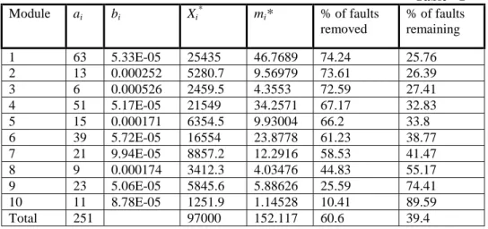
estimated using the software failure data. Consider a software having 10 modules whose parameter estimates are as given in Table-1. Suppose the total resource available for testing is 97000. First the problem (P1) is solved and from the recursion equation (7) optimal allocation of resources (Xi

*

that in some modules (module-9,10) the remaining faults after allocation is high. This can lead to frequent failure during operational phase. Obviously this will not satisfy the developer and he may desire that at least 50% of fault content from each of the modules of the Software is removed (i.e. pi=0.5 for each i = 1…10). Since faults in each module are integral values, nearest integer larger then 50% of the fault content in each module is taken as lower limit that has to be removed. The new allocation of resource along with expected number of fault removed, percentages of faults removed and faults remaining for each module after solving the problem (P2) through the problem (P5) is summarized in Table-2. The total number of faults that can be removed through this allocation is 146.8(i.e. 58.4% of the fault content is removed from the Software). In addition to the above if it is desired that a certain percentage of the total faults are to be removed then additional testing resources would be required. It is interesting to study this tradeoff and Table-3 summarizes results, where the required percentage of faults removed is 60%. To achieve this, 3000 units of additional testing effort is required. The total number of faults that can be removed through this allocation is 150.8(i.e. 60.09% of the fault content is removed from the Software). Analysis given in Tables-1, 2 and 3 help in providing the developer an insight into the resource allocation and the corresponding fault removal phenomenon and the objective can be set accordingly.

Table - 1

Module ai bi Xi* mi* % of faults

removed

% of faults remaining

1 63 5.33E-05 25435 46.7689 74.24 25.76

2 13 0.000252 5280.7 9.56979 73.61 26.39

3 6 0.000526 2459.5 4.3553 72.59 27.41

4 51 5.17E-05 21549 34.2571 67.17 32.83

5 15 0.000171 6354.5 9.93004 66.2 33.8

6 39 5.72E-05 16554 23.8778 61.23 38.77

7 21 9.94E-05 8857.2 12.2916 58.53 41.47

8 9 0.000174 3412.3 4.03476 44.83 55.17

9 23 5.06E-05 5845.6 5.88626 25.59 74.41

10 11 8.78E-05 1251.9 1.14528 10.41 89.59

Table-2

Module ai aio Zi* Yi* mi(Yi) mi* % of

faults removed

% of faults remaining

1 63 32 13300 7495.5 10.2 42 67 33

2 13 7 3064.6 1235.6 1.61 8 66.21 33.79

3 6 3 1317.3 672.1 0.89 4 64.89 35.11

4 51 26 13793 2969.7 3.56 30 57.96 42.04

5 15 8 4464.8 440.4 0.51 8 56.71 43.29

6 39 20 12565 0 0 20 51.28 48.72

7 21 11 7465.7 0 0 11 52.38 47.62

8 9 5 4652.5 0 0 5 55.56 44.44

9 23 12 14586 0 0 12 52.17 47.83

10 11 6 8978.1 0 0 6 54.55 45.45

Total 251 130 84187 12813.3 16.8 146 58.48 41.52

Table-3 Module ai aio Zi* Yi* mi(Yi) Xi* mi* % of

faults removed

% of faults remaining

1 63 32 13300 8624.7 11.74 21924.6 44 69.43 30.57 2 13 7 3064.6 1474.2 1.93 4538.82 9 68.7 31.3 3 6 3 1317.3 786.52 1.048 2103.79 4 67.47 32.53

4 51 26 13793 4134.5 5.13 17927.4 31 61.05 38.95

5 15 8 4464.8 793.16 0.984 5257.95 9 59.9 40.1

6 39 20 12565 0 0 12565.5 20 51.3 48.7

7 21 11 7465.7 0 0 7465.66 11 52.38 47.62

8 9 5 4652.5 0 0 4652.5 5 55.55 44.45

9 23 12 14586 0 0 14585.7 12 52.18 47.82

10 11 6 8978.1 0 0 8978.11 6 54.55 45.45

5.

Conclusion

In this paper we have discussed a couple of optimization problems occurring during module testing phase of software development life cycle. A dynamic programming approach for finding the optimal solution has been proposed. Using simple recursion equations it is shown how fault removal for each module and that of the software can be maximized, by judicious allocation of resources. It is observed that after certain duration of testing, fault removal becomes difficult in the sense that greater effort will be required to remove each additional fault. As the reliability of software is of utmost importance scientific decision making is required while deciding the resource budget. The tradeoff as shown in section-4 can be useful in this regard. Alternatively if the developer is not too keen on an optimal solution but is satisfied with an efficient solution, Goal Programming approach may be desirable in that case. We are further looking into this aspect.

Appendix:

Proof of the theorem-1

We have following recursion equations given in (7):

{

(

1

)

}

max

)

(

1 1

1

1

1 b X

Z X

e

a

Z

f

−

=

−

=

{

(

1

)

(

)

}

max

)

(

₁

0 n n

X b n

Z X

n

Z

a

e

f

Z

X

f

n n

n

−

+

−

=

− ₋

≤

≤ , n = 2, … , N

The above problem can be solved through forward recursion in N stages as follows. Stage-1: Let n=1 then we have

{

(

1

)

}

max

)

(

1 1

1

1

1 b X

Z X

e

a

Z

f

−

=

−

=

=

(

1

1

)

1

e

b Z

a

−

−

Stage-2: Let n=2 then we have

{

(

1

)

(

)

}

max

)

(

_{2 1 2}

2 0

2

Z

a

e

2 2

f

Z

X

f

b X

Z X

−

+

−

=

−

≤ ≤

Substituting f₁(Z−X₂) in above we have

{

(

1

)

(

1

)

}

max

)

(

_{2 1} ( )

2 0

2 b2X2 b1 Z X2

Z X

e

a

e

a

Z

f

− − −

≤

≤

−

+

−

Now let,

_F

₂

(

_X

₂

)

=

{

_a

₂

(

1

−

_e

−b2X2

)

+

_a

₁

(

1

−

_e

−b1(Z−X2)

)

}

_then

{

(

)

}

max

)

(

_{2 2}

2 0

2

Z

F

X

f

Z X ≤

≤

=

The maxima can be found through calculus. ) ( 1 1 2 2 2 2

2

(

)

b₂X₂ b₁ Z X₂

e

b

a

e

b

a

dX

X

dF

₌

−

₋

− −

The sufficiency condition can be checked through the second derivative condition:

0

)

(

_{2 ( )}

1 1 2 2 2 2 2 2 2 2 2 1 2

2

−

≤

−

=

_a

_b

_e

−b X

_a

_b

_e

−b Z−X

dX

X

F

d

The following three situations can occur.

(i)

(

)

0

2 2 2

_<

dX

X

dF

(ii)

(

)

0

2 2 2

₌

dX

X

dF

(iii)

(

)

0

2 2 2

_>

dX

X

dF

If ( ) ₀

2 2 2 _<

dX X

dF _{, then X}

2=0.

At X2=0

0

)

(

₁ 1 1 2 2 2 2

2

₌

_a

_b

₋

_a

_b

_e

−b Z

_<

dX

X

dF

i.e.

2

2

1

1

1

1

b

a

b

a

e

b

Z

<

≤

Which implies

a

₁

b

₁

>

a

₂

b

₂,in other words the detectability in module -1 is higher than module –2.

Similarly

(

)

0

2 2 2

_>

dX

X

dF

implies X2 = Z

and we have 2

1

1 1

2

2

_>

b Z

_≥

e

b

a

b

a

Hence

a

₂

b

₂

>

a

₁

b

₁, the testing resources would be allocated to module -2 first as the detectability is higher there.

Finally if

(

)

0

2

2

2

₌

dX

X

dF













−

+

=

∗ 2 2 1 1 1 2 1 2

log

1

b

a

b

a

Z

b

b

b

X

, i.e.













−

+

=

∗ 2 2 1 1 1 2 1 2

log

1

b

a

V

Z

b

X

µ

µ

and





















+

−

=

− + + =

∑

1 2

1 2 1 2 2 2 1 1

)

(

)

(

)

(

1 1 2 2 1 2 2 1 1 2 2 1

2 b b

b b b b Z b a b a i i

b

a

b

a

a

b

a

b

a

a

e

a

Z

f

i.e. ₂

2 1

2

(

Z

)

a

e

2

V

f

Z

i

i −µ

=

−

=

∑

Where 1 1 1

1

1

b

b

=

=

µ

, 1 1

a

V

=

,

2 1 2 1 2 1

2

₁

₁

1

b

b

b

b

b

b

+

=

+

=

µ





















+

=

2 2 1 2

)

(

)

(

1 1 2 2 1 2 2 1 1 2 2 b

V

b

a

V

b

a

V

a

V

µ µ µ

µ

µ

Now proceeding by induction it can be shown for nth stage,













−

+

=

₋ − − − ∗ n n n n n n n n

b

a

V

Z

b

X

₁ 1 1

1

log

1

_µ

µ

µ

and Z _n

n i

i

n

Z

a

e

V

f

−µn

=

−

=

∑

1

)

(

for n=1…N

The proof is complete.

References

1. Goel A.L., Software Reliability Models: Assumptions, limitations and applicability, IEEE Trans. On software engineering, SE-11, pp. 1411-1423, 1985.

2. Hadley, G., Nonlinear and Dynamic Programming, Addision-Wesley, Reading Mass, 1964.

3. Ichimori, T, Yamada, S. And Nishiwaki M., Optimal allocation policies for testing-resource based on a Software Reliability Growth Model, Proceedings of the Australia –Japan workshop on stochastic models in engineering, technology and management, pp. 182-189, 1993.

4. Kapur P.K. and Garg R.B.; Cost reliability optimum release policies for a software system with testing effort, OPSEARCH, vol. 27, no. 2, pp. 109-118, 1990.

6. Kapur, P.K. and Bardhan, A.K., Modelling, allocation and control of resources: an interdisciplinary approach in software reliability and marketing, Operations Research, Eds. M. Agarwal and K. Sen, Narosa Publishing House, New Delhi 2001.

7. Kubat P. and Koch H.S., Managing test procedures to achieve reliable software, IEEE Trans. On Reliability, Vol. R-32, pp. 299-303, 1983. 8. Musa J.D., Iannino A. And Okumoto K, Software

Reliability-Measurement, Prediction and Application, Mc Graw Hill, 1987.