Volume 2, Issue 4, April 2013
Abstract-Wireless sensor networks (WSNs) consist of a large number of sensor nodes that are densely deployed in a region of interest to collect data about a target or event, and to provide a variety of sensing and monitoring applications. Efficient design and implementation of wireless sensor networks has become a hot area of research in recent years, due to the vast potential of sensor networks to enable applications that connect the physical world to the virtual world. There are many characteristics that differs wireless network from wired network and these distinctions introduce the need for many different protocols of WSN at different layers i.e. Physical layer, Data Link layer, Network layer, Transport layer, Application layer. Many research works have been done on the design of low power electronic devices in order to reduce energy consumption of the sensor nodes of Wireless network. DSDV, AODV, DSR of Network Layer contribute to this factor in various ways. Advantages, Limitations and Comparison between DSDV, AODV and DSR protocols are discussed in detail throughout this paper.
Keywords: WSN , DSDV, AODV, DSR
I. INTRODUCTION
A routing protocol is a protocol that specifies how routers communicate with each other to disseminate information that allows them to select routes between any two nodes on a network. Typically, each router has a prior knowledge only of its immediate neighbors. A routing protocol shares this information so that routers have knowledge of the network topology at large. Wireless sensor network is one of the most considered factors of today’s world. Due to severe energy constraint of densely deployed network sensor nodes, to maintain network functions and management different routing techniques are needed. There are many techniques available for routing in wireless sensor network. Traditional techniques include- Flooding and Gossiping. In flooding a given node broadcasts data and control packets that it has received to the rest of the nodes in the network. This process repeats until the destination node is reached. Note that this technique does not take into account the energy constraint imposed by WSNs. As a result, when used for data routing in WSNs, it leads to the problems such as implosion which refers that-As flooding is a
blind technique, duplicating packets may keep circulate in the network, and hence sensors will receive those duplicate packet. To overcome this problem gossiping was introduced where a sensor would select randomly one of its neighbors and send the received packet to it. The same process repeats until all sensors receive this packet. Using gossiping, a given sensor would receive only one copy of a packet being sent. While gossiping tackles the implosion problem, there is a significant delay for a packet to reach all sensors in a network. Furthermore, these inconveniences are highlighted when the number of nodes in the network increases [1]. In this paper we have discussed about different routing protocols (DSDV, AODV, DSR), their significance in wireless sensor network and analyze the performance of these protocols using NS-2.
II. DESIGN ISSUES OF ROUTING PROTOCOL
The design of routing protocols in WSNs is influenced by many challenging factors. These factors must be overcome before efficient communication can be achieved in WSNs. In the following, we summarize some of the routing challenges and design issues that affect routing process in WSNs.
Node deployment:
Node deployment in WSNs is application dependent and affects the performance of the routing protocol. The deployment can be either deterministic or randomized. The sensors are manually placed and data is routed through pre-determined paths in deterministic deployment. However, in random node deployment, the sensor nodes are scattered randomly creating an infrastructure in an ad hoc manner [2]. If the resultant distribution of nodes is not uniform, optimal clustering becomes necessary to allow connectivity and enable energy efficient network operation. Inter-sensor communication is normally within short transmission ranges due to energy and bandwidth limitations. Therefore, it is most likely that a route will consist of multiple wireless hops.
Power Consumption:
Since the transmission power of a wireless radio is proportional to distance squared or even higher order in the presence of obstacles, multi-hop routing will consume less energy than direct communication. However, multi-hop routing introduces significant overhead for topology management and medium access control. Direct routing would perform well enough if all the nodes were very close to the sink. Sensor nodes are equipped with limited power
Performance analysis of DSDV, AODV and
DSR in Wireless Sensor Network
source (<0.5 Ah 1.2V).Node lifetime is strongly dependent on its battery lifetime.
Data Delivery Models:
Data delivery models determine when the data collected by the node has to be delivered. Depending on the application of the sensor network, the data delivery model to the sink can be Continuous, Event-driven, Query-driven and Hybrid [3]. In the continuous delivery model, each sensor sends data periodically. In event-driven models, the transmission of data is triggered when an event occurs. In query driven models, the transmission of data is triggered when query is generated by the sink. Some networks apply a hybrid model using a combination of continuous, event-driven and query-driven data delivery.
Node/Link Heterogeneity:
Although many applications of wireless sensor network rely on homogenous nodes, the introduction of different kinds of sensors could bring significant benefits. The use of nodes with different processors, transceivers, power units or sensing components may improve the characteristics of the network. Among other, the scalability of the network, the energy drainage or the bandwidths are potential candidates to benefit from the heterogeneity of nodes. For example, hierarchical protocols designate a cluster-head node different from the normal sensors. These cluster-heads can be chosen from the deployed sensors or can be more powerful than other sensor nodes in terms of energy, bandwidth, and memory. Hence, the burden of transmission to the BS is handled by the set of cluster-heads.
Fault Tolerance:
Some sensor nodes may fail or be blocked due to lack of power, physical damage, or environmental interference. The failure of sensor nodes should not affect the overall task of the sensor network. If many nodes fail, MAC and routing protocols must accommodate formation of new links and routes to the data collection base stations. This may require actively adjusting transmit powers and signaling rates on the existing links to reduce energy consumption, or rerouting packets through regions of the network where more energy is available. Therefore, multiple levels of redundancy maybe needed in a fault-tolerant sensor network.
Scalability:
The number of sensor nodes deployed in the sensing area may be in the order of hundreds or thousands, or more. Any routing scheme must be able to work with this huge number of sensor nodes. In addition, sensor network routing protocols should be scalable enough to respond to events in the environment. Until an event occurs, most of the sensors can remain in the sleep state, with data from the few remaining sensors providing a coarse quality.
Network Dynamics:
Most of the network architectures assume that sensor nodes are stationary. However, mobility of either BS’s or sensor nodes is sometimes necessary in many applications. Routing
messages from or to moving nodes is more challenging since route stability becomes an important issue, in addition to energy, bandwidth etc. Moreover, the sensed phenomenon can be either dynamic or static depending on the application, e.g., it is dynamic in a target detection/tracking application, while it is static in forest monitoring for early fire prevention. Monitoring static events allows the network to work in a reactive mode, simply generating traffic when reporting. Dynamic events in most applications require periodic reporting and consequently generate significant traffic to be routed to the BS.
Transmission Media:
In a multi-hop sensor network, communicating nodes are linked by a wireless medium. The traditional problems associated with a wireless channel (e.g., fading, high error rate) may also affect the operation of the sensor network. In general, the required bandwidth of sensor data will be low, on the order of 1-100 kb/s. Related to the transmission media is the design of medium access control (MAC). One approach of MAC design for sensor networks is to use TDMA based protocols that conserve more energy compared to contention based protocols like CSMA (e.g., IEEE 802.11). Bluetooth technology can also be used.
Connectivity:
High node density in sensor networks precludes them from being completely isolated from each other. Therefore, sensor nodes are expected to be highly connected. This, however, may not prevent the network topology from being variable and the network size from being shrinking due to sensor node failures. In addition, connectivity depends on the, possibly random, distribution of nodes.
Operating Environment:
In WSNs, each sensor node obtains a certain view of the environment. A given sensor's view of the environment is limited both in range and in accuracy; it can only cover a limited physical area of the environment. Hence, area coverage is also an important design parameter in WSNs.
Data Aggregation/Fusion:
Since sensor nodes might generate significant redundant data, similar packets from multiple nodes can be aggregated so that the number of transmissions would be reduced. Data aggregation is the combination of data from different sources by using functions such as suppression (eliminating duplicates), min, max and average [4]. As computation would be less energy consuming than communication, substantial energy savings can be obtained through data aggregation. This technique has been used to achieve energy efficiency and traffic optimization in a number of routing protocols.
Quality Of Service (Q o S):
Volume 2, Issue 4, April 2013
selection of routing protocols for a particular application. In some applications (e.g. some military applications) the data should be delivered within a certain period of time from the moment it is sensed.
Production Costs:
Since the sensor networks consist of a large number of sensor nodes, the cost of a single node is very important to justify the overall cost of the networks and hence the cost of each sensor node has to be kept low.
Data Latency And Overhead:
These are considered as the important factors that influence routing protocol design. Data aggregation and multi-hop relays cause data latency. In addition, some routing protocols create excessive overheads to implement their algorithms, which are not suitable for serious energy constrained networks.
Autonomy:
The assumption of a dedicated unit that controls the radio and routing resources does not stand in wireless sensor networks as it could be an easy point of attack. Since there will not be any centralized entity to make the routing decision, the routing procedures are transferred to the network nodes.
III. CLASSIFICATION OF ROUTING PROTOCOL
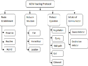
To classify Routing protocols a large number of characteristics, e.g. the routing technique, the route establishment procedure, and the protocol operation, and the generated network structure can be used. According to network structure, the routing protocols are categorized into flat, hierarchical, and location-based protocols. The protocol operation can be multi-path-based, query-based, negotiation-based, QoS-based, or coherent-based [5].The way the routing protocols establish routes in the network classifies them into three different categories. The first one is called proactive. A proactive protocol sets up routing paths and states before there is a demand for routing traffic. Paths are maintained even there is no traffic flow at that time. In reactive routing protocol, routing actions are triggered when there is data to be sent and disseminated to other nodes. Here paths are setup on demand when queries are initiated. The last group consists of hybrid protocols which combine the ideas of reactive and proactive route establishment. Routing protocols are also classified based on whether they are destination-initiated (Dst-initiated) or source-initiated (Src-initiated). Fig. 3.1 gives an overview of the routing taxonomy.
Route Establishment based routing protocol
Routing protocols can follow different strategies to enable connectivity between the nodes in the networks. Different strategies effects on the performance and lifetime of the network differently.
Three different route establishment strategies are available.
First one is proactive routing. Here, each node has one or more tables that contain the latest information of the routes to any node in the network. The proactive protocols are not suitable for larger networks, as they need to maintain node entries for each and every node in the routing table of every node. This causes more overhead in the routing table leading to consumption of more bandwidth. Examples of such schemes are the conventional routing schemes, Destination Sequenced Distance Vector (DSDV).
Figure 1: Taxonomy of Wireless Routing Protocol
Second routing protocol is Reactive protocol. These protocols do not maintain routing information or routing activity at the network nodes if there is no communication. If a node wants to send a packet to another node then this protocol searches for the route in an on-demand manner and establishes the connection in order to transmit and receive the packet. The route discovery usually occurs by flooding the route request packets throughout the network. Example of reactive routing protocol is ad hoc on-demand distance vector routing (AODV). Hybrid protocols use both reactive and proactive mechanisms to maintain existing routes or to establish new routes. Example of hybrid routing protocol is dynamic source routing (DSR). The majority of hybrid protocols can be divided into two groups. The first group does not transmit any routing information if no route is required. Only the source and the destination of an active route periodically transmit routing information in order to keep the existing routes up-to-date. The advantage of this approach compared to reactive strategies is that the routing protocol is able to quickly detect link breaks in active routes. The second group of hybrid protocols uses proactive routing mechanisms for short range communication and reactive routing techniques for long range communication. Thus, they use periodic broadcast mechanisms to establish and maintain routes to nodes which are reachable within two or three hops.
Network Structure based routing protocol
common network structures are flat, hierarchical, and location-based. In flat networks, each node typically plays the same role and sensor nodes collaborate together to perform the sensing task. Due to the large number of such nodes, it is not feasible to assign a global identifier to each node. This consideration has led to data centric routing, where the BS sends queries to certain regions and waits for data from the sensors located in the selected regions [6]. The main objective of hierarchical routing is to reduce energy consumption by classifying nodes into clusters. In each cluster, a node is selected as the leader or the cluster head. The different schemes for hierarchical routings mainly differ in how the cluster head is selected and how the nodes behave in the inter and intra-cluster domain [7].In section 3.3 we will discuss about LEACH elaborately which is a hierarchical routing protocol. Location-based protocols follow a different approach to structure the network. Nodes that are placed within a certain area are grouped instead of using a unique address for each node. Therefore, the networks scale with their size and not with the number of nodes.
Protocol Operation
Routing protocols can be also categorized with respect to their protocol operation. This kind of categorization has the advantage of being more application oriented compared to the two previously discussed taxonomies. In the following, the protocols are distinguished in negotiation-based and query-based protocols. Moreover, the protocols are grouped whether they offer multi-path or QoS support and depending on the used data processing technique. However, the protocol-based classification is not as strict as the other classifications. Thus, a routing protocol may fit into more than one category.
Initiator of Communicator
Routing protocols are also classified into destination-initiated (Dst-initiated)or source-initiated (Src-initiated). A source-initiated protocol sets up the routing paths upon the demand of the source node, and starting from the source node. Here source advertises the data when available and initiates the data delivery. A destination initiated protocol, on the other hand, initiates path setup from a destination node [8].
IV. DESTINATION-SEQUENCED DISTANCE-VECTOR ROUTING (DSDV)
The DSDV routing algorithm [Perkins 1994] is built on top of Bellman-Ford routing algorithm. There are two routing algorithms available. First one is Link-State algorithm each node maintains a view of the network topology and second one is Distance-Vector algorithm where every node maintains the distance of each destination. Distance-Vector algorithm is not suited for ad-hoc networks because it causes loops and count-to-infinity problem. The solution is to using DSDV protocol which is Destination Based and contains no global view of topology. In DSDV each node maintains routing information for all known destinations and routing
information must be updated periodically. The route labeled with the highest sequence number is always used. This also helps in identifying the stale routes from the new ones, thereby avoiding the formation of loops. DSDV allows fast reaction to topology changes. It makes immediate route advertisement on significant changes in routing table but waits with advertising of unstable routes (damping fluctuations).
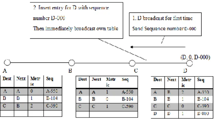
Figure 2: Table entries of DSDV routing protocol
Sequence number originated from destination. Ensures loop freeness.
Install Time when entry was made (used to delete stale entries from table)
Stable Data Pointer to a table holding information on how stable a route is. Used to damp fluctuations in network.
In DSDV each node advertises to each neighbor own routing information. These information are Destination Address, Metric (Number of Hops to Destination) and Destination Sequence Number. DSDV maintains some rules to set sequence number information. On each advertisement DSDV increases own destination sequence number (use only even numbers). If a node is no more reachable (timeout) then DSDV increases sequence number of this node by 1 (odd sequence number) and set metric = ∞.To minimize the traffic generated, there are two types of packets in the system. One is known as “full dump”, which is a packet that carries all the information about a change. However, at the time of occasional movement, another type of packet called “incremental” will be used, which will carry just the changes, thereby, increasing the overall efficiency of the system.
Volume 2, Issue 4, April 2013
Figure 4: DSDV (new node)
Figure 5: DSDV (no loops , no count to infinity)
Figure 6: DSDV (Intermediate Advertisement)
V. DSDV (FLUCTUATIONS AND SOLUTION OF FLUCTUATIONS)
If in case of Figure 1 we suppose that entry for D in A is [D, C, 14, D-100] and D makes Broadcast with Seq. Nr. D-102. If A receives from P Update (D, 15, D-102) then Entry for D in A, will be [D, P, 15, D-102], so A must propagate this route immediately. Again if A receives from P Update (D, 14,
D-102) then Entry for D in A, will be [D, Q, 14, D-102], so A must propagate this route immediately.
This can happen every time D or any other node does its broadcast and lead to unnecessary route advertisements in the network, so called fluctuations.
Figure 7: DSDV (Problem of Fluctuations)
To dump fluctuations some steps should be taken.
Record last
and avg. Settling Time of every Route in a separate table. (Stable Data)Settling Time = Time between arrival of first route and the best route with a given seq. nr.
A still must
update his routing table on the first arrival of a route with a newer seq. nr., but he can wait to advertising it. Time to wait is proposed to be 2*(avg. Settling Time).
Like this,
fluctuations in larger networks can be damped to avoid unnecessary advertisement, thus saving bandwidth.
Advantages of DSDV Routing Protocol:
DSDV protocol guarantees loop free paths.
Count to infinity problem is reduced in DSDV.
We can avoid extra traffic with incremental updates instead of full dump updates.
Path Selection: DSDV maintains only the best path instead of maintaining multiple paths to every destination. With this, the amount of space in routing table is reduced.
Limitations of DSDV Routing Protocol:
Wastage of bandwidth due to unnecessary advertising of routing information even if there is no change in the network topology.
DSDV doesn’t support Multi path Routing.
It is difficult to determine a time delay for the advertisement of routes.
It is difficult to maintain the routing table’s advertisement for larger network. Each and every host in the network should maintain a routing table
B
A
C
D
for advertising. But for larger network this would lead to overhead, which consumes more bandwidth.
VI. AD-HOC ON-DEMAND DISTANCE VECTOR (AODV) ROUTING
AODV is an “on demand routing algorithm”, meaning that it establishes paths only upon demand by source nodes. It maintains these paths as long as they are needed. Nodes that do not participate in active path neither maintain any routing information nor participate in any periodic routing table exchange. AODV established path based on route request- route reply mechanism.
Path Discovery Process:
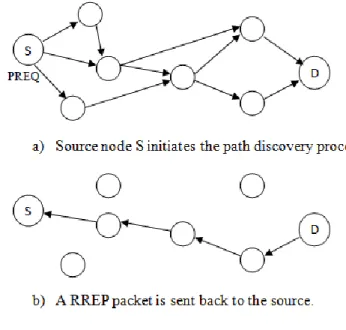
In order to discover the path, a route request message (RREQ) is broadcasted to all the neighbors which again continue to send the same to their neighbors, until the destination is reached. Every node maintains two counters: sequence number and broadcast-id in order to maintain loop-free and most recent route information. The Broadcast-id is incremented for every RREQ the source node initiates. If an intermediate node receives the same copy of request, it discards it without routing it further and if the neighboring nodes which receiving the RREQ has no route information about the destination then it will further broadcast RREQ packet in the network otherwise it will send answer by the route reply (RREP) packet to the sender from which RREQ is received. When a node forwards the RREQ message, it records the address of the neighbor from which it received the first copy of the broadcast packet, in order to maintain a reverse path to the source node. RREQ contains source address, source sequence number, broadcast_id, destination address, destination sequence number, and hop count broadcast_id uniquely identifies a RREQ, where broadcast_id is incremented when a new RREQ is issue by source.
Figure 8: Structure of a PREQ packet
Figure 9: Structure of a RREP packet
When the RREP reaches the source, the route is ready, and the initiator can use it. A neighbor that has communicated at least one packet during the past active timeout is considered active for this destination. An active entry in the routing table is an entry that uses an active neighbor. An active path is a path established with active routing table entries. A routing table entry expires if it has not been used recently. In this main content that AODV uses the route expiration technique, where a routing table entry expires within a specific period, after which a fresh route discovery must be initiated.
Figure 10: AODV Path Discovery Process
Maintaining Routes:
The nodes participating in an active route are notified by RERR (Route ERROR) packets when the next-hop link is down. The Route error propagation in AODV is achieved by all nodes participating in the route. Each one of them forwards the RERR to its predecessors. Consequently, all routing tables must be updated after this process. Nodes launches the RERR message in three cases: 1- detection of a link break for the next hop of an active route in its own routing table, 2- getting a data packet intended to a node that does not have an active route, 3- receiving a RERR from a neighbor in relation to one or more active routes. AODV uses the lifetime field to determine the expiry time for an active route. It also is also used to define the deletion time for an invalid route.
Figure 11: Structure of a RERR packet
Advantages of AODV Routing Protocol:
Reduces memory requirements and needless duplications
Volume 2, Issue 4, April 2013
Maintains loop-free routes by use of destination sequence numbers
Minimizes need for broadcast
Increases size of network depending on the number of nodes.
AODV for IPv6 is specified, built, and works
Limitations of AODV Routing Protocol:
The algorithm requires that the nodes in the broadcast medium can detect each others’ broadcasts.
Overhead on bandwidth will be occurred when an RREQ travels from node to node in the process of discovering the route info on demand, it sets up the reverse path in itself with the addresses of all the nodes through which it is passing and it carries all this info all its way.
AODV lacks an efficient route maintenance technique. The routing info is always obtained on demand, including for common case traffic.
The messages can be misused for insider attacks including route disruption, route invasion, node isolation, and resource consumption.
AODV is designed to support the shortest hop count metric. This metric favors long, low bandwidth links over short, high bandwidth links.
AODV does not discover a route until a flow is initiated. This route discovery latency result can be high in large-scale mesh networks.
VII. DYNAMIC SOURCE ROUTING (DSR)
DSR maintains some mechanism for routing packets. Firstly, to send a packet to another host, the sender constructs a source route in the packet’s header, giving the address of each host in the network through which the packet should be forwarded in order to reach the destination host. The sender then transmits the packet according to the route. When a host receives a packet, if this host is not the final destination of the packet, it simply transmits the packet to the next hop identified in the source route in the packet’s header. Once the packet reaches its final destination, the packet is delivered to the network layer software on that host.
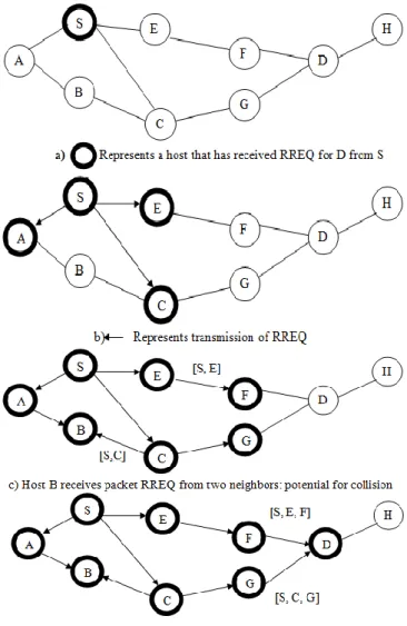
Secondly, while sending packet from one host to another, if the route is not found, the sender may attempt to discover one using the route discovery mechanism. If host S is source host and D is destination host and S initiates a route discovery in absence of route. Source host S floods Route Request (RREQ). Each host appends own identifier when forwarding RREQ.
Figure 12: Route Discovery of DSR
Figure 13: Route Reply of DSR
Thirdly, while a host is using any source route, it monitors the continued correct operation of that route. For example, if the sender, the destination, or any of the other hosts named hops along a route move out of wireless transmission range of the next or previous hop along the route, the route can no longer be used to reach the destination. A route will also no longer of work if any of the hosts along the route should fail or be powered off. This monitoring of the correct operation of a route in use we call route maintenance. When route maintenance detects a problem with a route in use, route discovery may be used again to discover a new, correct route to the destination.
Fourthly, each mobile host participating in the ad hoc network maintains a route cache in which it caches source routes that it has learned. When one host sends a packet to another host, the sender first checks its route cache for a source route to the destination. If a route is found, the sender uses this route to transmit the packet.
Advantages of DSR:
Routes maintained only between nodes who need to communicate
o reduces overhead of route maintenance
Route caching can further reduce discovery overhead
A single route discovery may yield many routes to the destination, due to intermediate nodes replying from caches
Disadvantages of DSR:
Packet header size grows with route length due to source routing
Flood of route requests may potentially reach all nodes in the network
Potential collisions between route requests propagated by neighboring nodes
o Insertion of random delays before forwarding RREQ
Stale caches will lead to increased overhead
Increased contention if too many route replies come back due to nodes replying using their local cache
o Route Reply Storm problem
VIII. COMPARISON AND EVALUATION
In this section, we compare the three routing protocol: DSDV, AODV and DSR, discussed previously. We have used simulation results to compare the protocols.
IX. SIMULATION MODEL
The experiments use a fixed number of packet sizes (512-bytes). The mobility model used is a radio propagation model. The field configurations used is 500m X 500m with different number of nodes. Here, each packet starts its journey from a random location to a random destination with a randomly chosen speed. Simulation runs for 100 simulated seconds. Identical mobility and traffic scenarios are used across protocols to gather fair results.
The Wireless scenario for this experiment looks like:
Figure 14: NAM output
X. Performance Metrics
We focus on two performance metrics which are quantitatively measured. The performance metrics are important to measure the performance and activities that are running in NS-2 simulation. The performance metrics are:
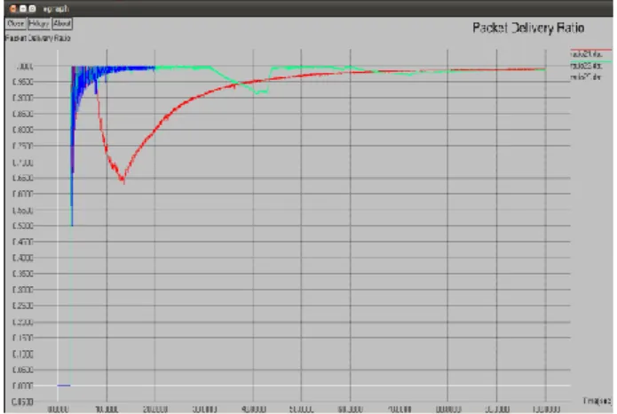
a) Packet delivery fractions (PDF): the ratio of the data packets delivered to the destinations to those generated by the CBR sources. The PDF shows how successful a protocol performs delivering packets from source to destination. The higher for the value give use the better results. This metric characterizes both the completeness and correctness of the routing protocol also reliability of routing protocol by giving its effectiveness.
Packets received by the destination node Packet Delivery Ratio=
Packets sent
Volume 2, Issue 4, April 2013
a) Packet Delivery Fraction
Figure 15(a): Packet Delivery Fraction of DSDV, AODV, DSR with 20 nodes
Figure 15(b): Packet Delivery Fraction of DSDV, AODV, DSR with 30 nodes
Figure 15(c): Packet Delivery Fraction of DSDV, AODV, DSR with 40 nodes
Figure 15(d): Packet Delivery Fraction of DSDV, AODV, DSR with 50 nodes
Figure 15(a), 15(b), 15(c), 15(d) shows the Xgraph for AODV, DSDV and DSR with nodes 20, 30, 40 and 50 respectively where red curve is for DSDV, green one is for AODV and blue is for DSR. The X-axis of the graph indicates the time and the Y-axis shows the Packet Delivery Fraction. Based on these Figures it is shown than AODV perform better as we know when the number of nodes increases, nodes become more stationary which will lead to more stable path from source to destination in case of AODV. That’s why the output curve for AODV is high having slight change in all the plotting above. DSDV performance dropped as number of nodes increase because more packets dropped due to link breaks. That’s why the curve for DSDV fluctuates so much. In figure 15 (a) it is high but in figure 15(b) it suddenly drops and increases with time, then again for node 40 it becomes high and for node 50 it drops slightly and starts to rise with the advancement of time. DSR curve in all the figures acts same as AODV.
b) Throughput
Figure 16(a): Throughput comparison with 20 connections
is AODV and blue is for DSR. The X-axis of the graph indicates the time and the Y-axis shows the throughput. As we can clearly observe from the graph, the throughput of AODV and DSR is better than DSDV. There is a steady increase of throughput in case of AODV and DSR whereas in case of DSDV it is not the same. Thus in case of Throughput, AODV performs well when compared to DSDV.
Figure 16(b): Throughput comparison with 30 connections
The above figure shows the Xgraph for AODV, DSDV and DSR with 30 connections. The X-axis of the graph indicates the time and the Y-axis shows the throughput. From this figure also we can see that throughput for AODV and DSR are better than DSDV.
The reason for this difference is the wastage of bandwidth in case of DSDV due to unnecessary advertising of routing information even if the network is in idle mode. That’s why throughput for DSDV rises at time 0.0000 then gradually decreases with the advancement of time.
REFERENCES
[1] Shio Kumar Singh, M P Singh, and D K Singh, “Routing Protocols in Wireless Sensor Networks –A Survey”, International Journal of Computer Science & Engineering Survey (IJCSES) Vol.1, No.2, November 2010.
[2] Alexander Klein, “Performance Issues of MAC and
Routing Protocols in Wireless Sensor Networks, PhD thesis, University of Würzburg,
December 2010.
[3] Kemal Akkaya , Mohamed Younis, “A survey on routing protocols for wireless sensor networks”, Ad Hoc Networks 3 (2005) 325–349
[4] S. Tilak et al., A taxonomy of wireless microsensor
network models, Mobile Computing and
Communications Review 6 (2) (2002) 28–36.
[5] B. Krishnamachari, D. Estrin, S. Wicker, Modeling data centric routing in wireless sensor networks, in: Proceedings of IEEE INFOCOM, New York, June 2002. [6] Jamal N. Al-Karaki, Ahmed E. Kamal, “Routing Techniques in Wireless Sensor Networks: A Survey”,
Year-2004, IEEE Wireless Communications, Pages: 6-28, volume-11.
[7] Luis Javier García Villalba, Ana Lucila Sandoval Orozco, Alicia Triviño Cabrera and Cláudia Jacy Barenco Abbas, “Routing Protocols in Wireless Sensor Networks”, Journal: Sensors, Year: 2009, Vol: 9, Issue: 11, Pages/record No.: 8399-8421.
[8] Rajashree.V.Biradar, V.C .Patil, Dr. S. R. Sawant, Dr. R.
R. Mudholkar, “CLASSIFICATION AND
COMPARISON OF ROUTING PROTOCOLS IN
WIRELESS SENSOR NETWORK”, Ubiquitous
Computing and Communication Journal, Special Issue on Ubiquitous Computing Security Systems, Volume:
Ubiquitous Computing Security Systems
Publishing Date: 8/20/2009.
Nasrin Hakim Mithila has received B.Sc.