Assessing Software Reliability Using Exponential Imperfect
Debugging Model
B Prameela Rani , A. Srisaila , K. Sita Kumari, M.V.D.N.S.Madhavi Student, Department of Information Technology, V.R Siddhartha Engineering college
Asst. Professor,Department of Information TechnologyV. R .Siddhartha Engg .College [email protected]
Assoc. Professor,Department of Information TechnologyV. R. Siddhartha Engg. College [email protected]
Asst. Professor, Department of Mathematics, V. R .Siddhartha Engg .College [email protected]
ABSTRACT
Software reliability is one of the most important characteristics of software quality. As the usage of software reliability is growing rapidly, accessing the software reliability is a critical task in development of a software system. So, many Software Reliability Growth Models (SRGM) are used in order to decide upon the reliable or unreliable of the developed software very quickly. The well known software reliability growth model called as Exponential Imperfect Debugging model is a two parameter Non Homogeneous Poisson Process model which is widely used in software reliability growth modeling. In this paper, we propose to apply Statistical Process Control (SPC) to monitor software reliability process. A control mechanism is proposed based on the cumulative observations of failures which are grouped using mean value function of the Exponential Imperfect Debugging model. The Maximum Likelihood Estimation (MLE) approach is used to estimate the unknown parameters of the model. The process is illustrated by applying to real software failure data.
Keywords: Exponential Imperfect Debugging model, Non Homogeneous Poisson Process, Maximum Likelihood Parameter Estimation, SPC.
1. INTRODUCTION
Software Reliability is the application of statistical techniques to data collected during system development and operation to specify, predict, estimate, and assess the reliability of software based systems. To identify and eliminate errors in software development process and also to improve software reliability, the Statistical Process Control
concepts and methods are the best choice. SPC concepts and methods are used to monitor the performance of a software process over time in order to verify that the process remains in the state of statistical control. It helps in finding assignable causes, long term improvements in the software process. Software quality and reliability can be achieved by eliminating the causes or improving the software process or its operating procedures [2].
The most popular technique for maintaining process control is control charting. Software process control is used to secure the quality of the final product which will conform to predefined standards. In any process, regardless of how carefully it is maintained, a certain amount of natural variability will always exist. A process is said to be statistically
“in-control” when it operates with chance causes of variation. On the other hand, when assignable causes
are present, the process is statistically “out
variability of the process to be controlled. The early detection of software failures will improve the software reliability. The selection of proper SPC charts is essential to effective statistical process control implementation and use. The SPC chart selection is based on data, situation and need [4]. Many factors influence the process, resulting in variability. The causes of process variability can be broadly classified into two categories, viz., assignable causes and chance causes.
The control limits for the chart are defined in such a manner that the process is considered to be out of control when the time to observe exactly one failure is less than LCL or greater than UCL. Our aim is to monitor the failure process and detect any change of the intensity parameter [10].
2. LITERATURE SURVEY
This section presents the theory that underlies exponential imperfect distribution and maximum likelihood estimation for complete data. If
“t” is a continuous random variable with pdf:
f(t; , , , , … . . ).where
, , , , … . . unknown constant
parameters which need to be estimated, and cdf: F(t).where the mathematical relationship between the
pdf and cdf is given by :f(t)=( ( ( ))).Let “a” denote
the expected number of faults that would be detected given infinite testing time in case of finite failure NHPP models. Then, the mean value function of the finite failure NHPP models can be written as: m(t)=aF(t).Where, F (t) is a cumulative distribution function. The failure intensity function λ(t) in case
of the finite failure NHPP models is given by:
λ(t)=a ( )[9].
2.1 NHPP MODEL
Non-Homogenous Poisson Process (NHPP) based software reliability growth models (SRGMs) are proved to be quite successful in practical software reliability engineering. The main issue in the NHPP model is to determine an appropriate mean value function to denote the expected number of failures experienced up to a certain time point. Model parameters can be estimated by using Maximum Likelihood Estimate (MLE). Various NHPP SRGMs have been built upon various assumptions. Many of the SRGMs assume that each time a failure occurs, the fault that caused it can be immediately removed and no new faults are introduced. Which is usually called perfect debugging. Imperfect debugging models have proposed a relaxation of the above assumption.
2.2 EXPONENTIAL IMPRFECT DEBUGGING MODEL
The exponential imperfect debugging model is the non-homogenous Poisson process (NHPP) based on software reliability growth model. Then Non-homogeneous Poisson process (NHPP) based (SRGM) are proved to be quite successful in practical software reliability engineering. The main issue in the NHPP model is to determine an appropriate mean value function to denote the expected number of failures in interval domain data.
The exponential imperfect debugging model is adopted for interval domain data based on non-homogeneous Poisson process (NHPP) which is used in accessing the reliability of developed software. Let {N (t), t>=0} be the cumulative number of software failures bytime‘t’. m(t) is the mean value function, representing the expected number of software failures
by time ‘t’.
Thus
( )
[1
(1 )]
1
bt
a
m t
e
where “a” denotes the initial number of faults contained in a program and “b” represents the
fault detection rate. In software reliability, the initial number of faults and the fault detection rate are always unknown.
2.3 MAXIMUM LIKELIHOOD ESTIMATION
In much of the literature the preferred method of obtaining parameter estimates is to use the maximum likelihood equations. Likelihood equations are derived from the model equations and the assumptions which underlie these equations. The parameters are then taken to be those values which maximize these likelihood functions. These values are found by taking the partial derivate of the likelihood function with respect to the model parameters, the maximum likelihood equations, and setting them to zero. Iterative routines are then used to solve these equations. Unfortunately, the SRGM literature is sadly lacking in advice on which iterative routines to use, and with what starting values. This is unfortunate because the accuracy of parameter estimates and thus the accuracy of the models themselves greatly depend on the ability of the iterative search methods used to overcome local minima and find good values for the parameters. If we conduct an experiment and obtain N independent observations, , , ,… . .
The likelihood function may be given by the following product:
1) 1 1
(
.log[ ( )
(
)]
( )
n
i i i i n
i
LLF
y
y
m t
m t
m t
3. PARAMETER ESTIMATION
In this section we develop expressions to estimate the parameters of the Exponential Imperfect Debugging model based on interval domain data. Parameter estimation is of primary importance in software reliability prediction.
A set of failure data is usually collected in one of two common ways, time domain data and interval domain data. In this paper parameters are estimated from the interval domain data.
In interval domain assuming that the data are given for the cumulative number of detected
errors
i
y
in a given time interval (0,t
i) where i= 1,2. .. , n and 0 < t1 < t2< ... <
t
n, then the log likelihood function (LLF) takes on the following form:1) 1
1
(
.log[ ( )
(
)]
( )
n
i i i i n
i
LLF
y
y
m t
m t
m t
3.1.EXPONENTIAL IMPERFECT DEBUGGING MODEL BASED ON INTERVAL DOMAIN FAILURE DATA
The mean value function of Exponential Imperfect Debugging model is given by
(1 )
( )
[1
]
1
bt
a
m t
e
Assuming that the data are given for the cumulative number of detected errors
i
y
in a given time interval(0,
t
i) where i= 1, 2. .. , n and 0 < t1 < t2< ... <t
n, then the log likelihood function (LLF) takes on the following form:1) 1
1
(
.log[ ( )
(
)]
( )
n
i i i i n
i
LLF
y
y
m t
m t
m t
The likelihood function of Exponential Imperfect Debugging model for interval domain data is given as,
1) 1
1
(
.log[ ( )
(
)]
( )
n
i i i i n
i
LLF
y
y
m t
m t
m t
…..(3.1.1)
Therefore
(1 )
( )
[1
]
1
bt
a
m t
e
…..(3.1.2)
By substituting the value of m(t) in equation, we get
1
(1 ) (1 ) (1 ) 1
1
( ) log[ [1 1 ] [1 ]
1 1
i ti n
n
bt b bt
i i i
a a
LLF y y e e e
. .... (3.1.3)
1
(1 ) (1 ) (1 ) 1
1
( ) log[ ( )] [1 ]
1 1
i i n
n
bt bt bt
i i i
a a
LLF y y e e e
..…(3.1.4)
Partially differentiating with respect to ‘a’ and equating to ‘0’
(1 )
1 1
1
[1
]
(
).
1
n bt n i i iL
e
y
y
a
a
0
L
a
1 (1 )
1
1
]
(
).
1
nn
i i bt
i
a
y
y
e
…..(3.1.5)By substituting the value of ‘a’ in LL
1 (1 ) (1 ) (1 )
1 1
1 1
( ).[ log n log( i i)] ( )
n n
bt bt bt
i i i i
i i
LLF y y e e e y y
…(3.1.6)
Partially differentiating with respect ‘b’ and equals to ‘0’
1
1
(1 ) ) (1 ) 1
1 (1 ) (1 ) )
1
(1 )[ ]
( ). (1 )
i i
i i i
bt bt
n
i i
i n bt bt
i
t e t e
L
y y t
b e e
…..(3.1.7)Again partially differentiating with respect
‘b’ and equals to ‘0. Then we get
1
1
(1 ) ( )
2
2 1
1 (1 ) (1 ) ) 2
1
[ ( ) .
( ) ( )(1 )
( )
i i
i i
b t t
n
i i
i i bt bt
i
t t e
g b y y
e e
.…(3.1.8)4. INTERVAL DOMAIN FAILURE DATA SETS
Data Set #1:Phase1 Test data Week
Index
Exposure time (cum system test hours)(ti)
Fault (fi) Cum. Fault
(fi)
1 356 1 1
2 712 0 1
3 1068 1 2
4 1424 1 3
5 1780 2 5
6 2136 0 5
7 2492 0 5
8 2848 3 8
9 3204 1 9
10 3560 2 11
11 3916 2 13
12 4272 2 15
13 4628 4 19
14 4984 0 19
15 5340 3 22
16 5696 0 22
17 6052 1 23
18 6408 1 24
19 6764 0 24
20 7120 0 24
21 7476 2 26
Table 4.1:Phase1 test data
Data Set #2:Phase2 Test data Week
Index
Exposure time (cum system test hours)(ti)
Fault (fi) Cum.
Fault (fi)
1 416 3 3
2 832 1 4
3 1248 0 4
4 1664 3 7
5 2080 2 9
6 2496 0 9
7 2912 1 10
8 3328 3 13
9 3744 4 17
10 4160 2 19
11 4576 4 23
12 4992 2 25
13 5408 5 30
14 5824 2 32
15 6240 4 36
16 6656 1 37
17 7072 2 39
18 7488 0 39
19 7904 0 39
20 8320 3 42
21 8736 1 43
Table 4.2: Phase2 data set
Data Set #3: WOOD (1996) release2 data set
Test week CPU hours Defects found
1 519 16
2 968 24
3 1430 27
4 1893 33
5 2490 41
6 3058 49
7 3625 54
8 4422 58
9 5218 69
10 5823 75
11 6539 81
12 7083 86
13 7487 90
14 7846 93
15 8205 96
16 8564 98
17 8923 99
18 9282 100
19 9641 100
20 10000 100
Table 4.3: Wood (1996) Release1 data set
Data Set #4: WOOD (1996) release2 data set Test week CPU hours Defects found
1 384 13
2 1186 18
3 1471 26
4 1471 34
5 2236 40
6 2772 48
7 2967 61
8 3812 75
9 4880 84
10 6104 89
11 6634 95
12 7229 100
13 8072 104
14 8484 110
16 9712 114
17 10083 117
18 10174 118
19 10272 120
20 … ….
Table 4.4: Wood (1996) Release 2 data set
4.1 CALCULATION OF RELIABILITY FOR EXPONENTIAL IMPERFECT DEBUGGING MODEL:
Solving equations in section 3.1 by Newton Raphson Method (N-R) method for the Phase 1 test data, the iterative solutions for MLEs of a, and b and are
a^=23.7
b^=0.00997 Hence, we may accept these two values as MLEs of a, and b. The estimator of the reliability
function from the equation (3.1) at any time x beyond 7476 hours is given by
[ ( ) ( )]
( /
)
m s x m sR S X
e
[ (712 1068) (712)]
( /
)
m mR S X
e
=0.977.4.2 ESTIMATED PARAMETERS AND THEIR CONTROL LIMITS
The estimated parameters and the calculated control limits of the Failure control Chart for Data Set#1, Data Set #2, Data Set #3 and Data Set #4 with the false alarm risk, ᵦ = 0.05 are given in Tables. Using the estimated parameters and the estimated limits, we calculated the control limits we calculated the control limits UCL= m(tu),CL= m(tc)
and LL= m(tL).They are used to find whether the
software process is in control or not. The estimated
values of ‘a’ and ‘b’ and their control limits are as follows.
Therefo
(1 )
( )
[1
]
1
bt
a
m t
e
Where Tu=0.99865
Tc=0.05
TL=0.00135
Where = 0.05, b=0.0090, a=38
Substitute the above values and Tu ,Tc, TL values are in place of ‘t’ in mean m(t).
Then we get the values Tu=313.6219649
Tc=68.04329
TL=0.13736
These limits are converted to m(tu), m(tc)
and m(tL) by using SPC and by substituting the
values are a=38.0 , b=0.0090 and Tu, Tc, TL in mean
m(t).Then we get control limits.
DATA SET
ESTIMAT ED PARAMET
ERS
CONTROL LIMITS
a b m(tu) m(tc) m(tL)
Phase1
Test data 23.7 0.00
97 23.66 7
11.851 3
0.0324 3
Phas2
Test data 38.0 0.00
90
37.94 92
18.937 8
0.0519 2 Wood1
Data Set 79.8 0.03
00 79.69 39.8
0.1074 5 Wood2
Data Set 101.
65
0.03 075
101.5
12 50.82 0.0453
Table 4.2.1: Parameter estimates and Control limits
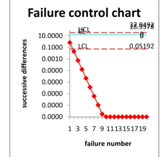
5. DISTRIBUTION OF INTERVAL DOMAIN DATA FAILURES
The mean value successive differences of time between failures cumulative data of the considered data sets are tabulated in Table 4.1 and 4.2. Considering the mean value successive differences on y axis, failure numbers on x axis and the control limits on Failure control chart, we obtained figure 5.1 and 5.2 . A point below the control limit m(tL) indicates an alarming signal. A
point above the control limit m(tu) indicates better
quality. If the points are falling within the control limits it indicates the software process is in stable.
S.N O
CUM.
FAILURE m(t) SD
S
2 712 24.917974 0.02838573
3 1068 24.946359 0.00097436
4 1424 24.947334 3.34461E
5 1780 24.947367 1.14807E
6 2136 24.947368 -2.35929967
7 2492 22.588069 2.3592997
8 2848 24.947368 4.6434E
9 3204 24.947368 1.59517E
10 3560 24.947368 5.32907E
11 3916 24.947368 0
12 4272 24.947368 0
13 4628 24.947368 0
14 4984 24.947368 0
15 5340 24.947368 0
16 5696 24.947368 0
17 6052 24.947368 0
18 6408 24.947368 0
19 6764 24.947368 0
20 7120 24.947368 0
21 7476 24.947368
Table 5.1: Successive differences of mean values, Phase1 Test Data
Fig 5.1: Failure control chart of Phase1 Test Data
S.NO CUM.
FAILURES m(t) SD
1 416 24.23562 0.6914416
2 832 24.927062 0.0197268
3 1248 24.946789 0.00056280
4 1664 24.947352 1.60568
5 2080 24.947368 4.58101
6 2496 24.94736 1.30696
7 2912 24.94736 3.72875
8 3328 24.23562 3.72875
9 3744 24.23562 1.06404
10 4160 24.23562 3.05533
11 4576 24.946789 0
12 4992 24.946789 0
13 5408 24.946789 0
14 5824 24.946789 0
15 6240 24.946789 0
16 6656 24.946789 0
17 7072 24.946789 0
18 7488 24.946789 0
19 7904 24.946789 0
20 8320 24.946789 0
21 8736 24.946789
Table 5.2: Successive differences of mean values, Phase2 Test Data
Fig 5.2: Failure control chart of Phase2 Test data
CONCLUSION:
The analysis shows that WOOD (1996) RELEASE 1 data is more reliable than all other datasets. The Exponential Imperfect Debugging Model got best results. The given interval domain data failures are plotted through the estimated mean value function against the failure serial order. The graphs have shown out of control signals i.e. below LCL. When the control signals are below LCL, it is likely that there are assignable causes leading to significant process deterioration and it should be investigated By observing the Control chart it is Identified that, for DS#1(fig 5.1) the failure process out of LCL the failure situation is detected at 5thpoint below LCL. For DS#2 (fig 5.2) the failure situation is detected at 8thpoint below LCL. Hence our proposed Control Chart detects out of control situation. When the control signals are below LCL, it is likely that there are assignable causes leading to significant process deterioration and it should be investigated .Hence we conclude that our method of estimation and the control chart are giving a positive recommendation for their use in finding out
UCL 23.60000
CL 11.85130
LCL 0.03243
-2.4055 7.5945 17.5945 27.5945
1 3 5 7 9 11 13 15 17 19
su
cc
es
siv
e
di
ffe
re
nc
es
failure number
Failure control chart
UCL 37.94920 CL 18.93780
LCL 0.05192
0.0000 0.0000 0.0000 0.0000 0.0000 0.0010 0.1000 10.0000
1 3 5 7 9 1113151719
su
cc
es
siv
e
di
ffe
re
nc
es
failure number
preferable control process or desirable out of control signal. The early detection of software failure will improve the software reliability.
FUCTURE WORK:
Software Reliability is assessed with Exponential Imperfect debugging model by estimating the parameters using Maximum likelihood method for interval domain data. This project can be extended by applying Sequential Probability Ratio Test (SPRT) for interval domain data.
REFERENCES
1. Agresti, a(1990) categorical data analysis. Wile,
new York , “standard glossary of software engineering terminology”.
2. kimura, M.,yamuda, s. osaki, s., “statistical
software reliability prediction and its applicability
based on mean time between failures”.
3. MacGregor, J.F., Kourti, T., “Statistical process control of multivariate processes”. Control
Engineering Practice Volume 3, Issue 3, March 1995, 403-414.
4. Anderson T, Lee P (1980) Fault Tolerance: Principles and Practices, Prentice-Hall, Englewood Cliffs.
5. Koutras, M.V., Bersimis, S., Maravelakis,P.E.,
“Statistical process control using shewart control charts with supplementary Runs rules” Springer
Science + Business media 9: 2007. 207-224.
6. MacGregor, J.F., Kourti, T., “Statistical process control of multivariate processes”. Control
Engineering Practice Volume 3, Issue 3, March 1995, 403-414.
7. Anderson T, Lee P (1980) Fault Tolerance: Principles and Practices, Prentice-Hall, Englewood Cliffs.
8. Anderson T, Barrett P, Halliwell D, Moulding M
(1985) “Software fault tolerance: An evaluation,”
IEEE Transactions on Software Engineering, vol SE-11(12).
9. Anderson T, Barrett P, Halliwell D, Moulding M
(1985) “Software fault tolerance: An evaluation,”
IEEE Transactions on Software Engineering, vol SE-11(12).
10. Tohma Y, Yamano H, Ohba M, Jacoby R (1991) "The estimation of parameters of the hypergeometric distribution and its application to the software reliability.
11. Growth model,“ IEEE Trans. Software Engineering, vol. SE-17(5) Tokuno K, Yamada S (1997) "Markovian availability measurement and assessment for hardware-software systems,“ Int. J Reliability, Quality and Safety Engineering,Vol. 4(3). 12. Swapna S. Gokhale and Kishore S.Trivedi, “Log
-Logistic Software Reliability Growth Model”. The
3rd IEEE International Symposium on High-Assurance Systems Engineering. IEEE Computer Society. 1998.
13. S. S. Gokhale and K. S. Trivedi, “A
time/structure based software reliability model”,