Accredited by RISTEKDIKTI, Decree No: 32a/E/KPT/2017
doi: 10.14203/jet.v18.27-34
Analysis of Non Linear Frequency Modulation (NLFM)
Waveforms for Pulse Compression Radar
Muhamad Ridwan Widyantara
a, *, Sugihartono
a, Fiky Y. Suratman
a,
Slamet Widodo
b, Pamungkas Daud
ba Faculty Electrical Engineering
Telkom University (TEL-U)
Jl. Telekomunikasi No. 01, Terusan Buah Batu, Sukapura, Dayeuhkolot Bandung, Indonesia
b Research Center for Electronics and Telecommunications (PPET)
Indonesian Institute of Sciences (LIPI) Kampus LIPI Gd.20, Lt. 4, Jl.Sangkuriang
Bandung, Indonesia
Abstract
Non Linear Frequency Modulation (NLFM) method can suppress the peak sidelobe level without additional windowing function. NLFM doesn’t require any weighting function because it has inbuilt one. NLFM has a variable frequency deviation function due to the relation between frequency and time of the signal which is not linear so that it is possible to suppress of peak sidelobe level. This paper studies the characteristic of various NLFM waveform, such as NLFM Tri Stage Piece Wise (TSPW), NLFM S, and NLFM Taylor. The study of Pulse Compression of NLFM waveform consists of three aspects. First, analysis of pulse compression performance. Second, analysis of background noise. Last, analysis of Doppler effects. The simulation is done using Matlab software. The lowest value Peak Sidelobe Level (PSL)of NLFM TSPW is about -20 dB while NLFM S and NLFM Taylor are about -32 dB and -39 dB. Additive White Gaussian Noise (AWGN) and Doppler Effect influenced the value of PSL for each NLFM waveform. NLFM Taylor has the best NLFM waveform when the Doppler Effect and AWGN cause the value of PSL become high. Comparison between NLFM Taylor and Linear Frequency Modulation(LFM) is done in radar surveillance applications to analyze the detectability performance where the condition of Radar Cross Section (RCS) for each target has different significant value. The three targets are commercial airplanes, helicopter and fighter. For detectability performance, NLFM Taylor can detect more clearly than LFM conventional.
Keywords: NLFM, LFM, PSL, Pulse Compression Radar, Doppler Effect.
I. INTRODUCTION
A good radar system can detect two or more long distance targets [1], where the distance between each target is very close. The parameter of range resolution in radar system will be separating the closely spaced of targets and it relates to the pulse width of the waveform [2]. Waveform design of radar is importance for radar performance. Two important parameters in waveform design are detection of maximum range and resolution of radar [3]. Power transmits will influence the detection range of radar. Increasing the power transmits improves the range of radar detection but this conventional method required large power supply, large dimension, safety and reliability problem [1], [4]. The high resolution radar can be achieved by narrowing the pulse width of the coming signal from the object reflection. But if the pulse width decreases, the amount of energy in the pulse decreases as well and reduces maximum range detection [2]. To solve the problem between parameters of detection and parameter of resolution, pulse compression is used in the radar systems.
Pulse compression is a technique for transmitting pulses with long durations, so the high energy of the pulse can be maintained to obtain the maximum detection while compression process is done in the receiver to produce a much narrower pulse width to make high resolution in the radar. In pulse compression technique, the echo signal at the radar receiver, pass through the matched filter to maximize the output of signal to noise ratio (SNR) [3]. Various methods have been developed for pulse compression to improve radar performances. The waveform design of pulse compression is usually using frequency or phase modulation [5]. LFM is pulse compression type which is commonly used in current radar systems because of its simplicity and Doppler tolerant [6]. However, this method has a drawback in its high sidelobe level, the matched-filtered response of this waveform has a peak sidelobe level about -13dB from the mainlobe level [7]-[9]. The high PSL decreases the radar detectability especially on the weak echoes of the target [6]. One of the solutions to reduce sidelobe level of LFM is required weighting function for pulse compression. Hamming, Kaiser and Chebyshev are the weighting function that can reduce the sidelobe level of pulse compression but it will reduce the parameter of SNR [10]. NLFM is another pulse compression technique to overcome this lack [6], [7], [9], [11]. NLFM waveforms
* Corresponding Author.
Email: [email protected]
Received: February, 01 2018 ; Revised: April, 20 2018 Accepted: May, 04 2018 ; Published: August, 31 2018
can achieve the good range resolution and at the same time has low PSL without additional windowing. NLFM doesn’t require any weighting function because they have inbuilt one [9]. This paper studies some waveform of NLFM to improve the performance of radar pulse compression. This paper compared and evaluated some types of NLFM waveform, which are NLFM TSPW, NLFM S and NLFM Taylor. And then evaluated some parameters assessment of the NLFM waveform to improve the performance of radar pulse compression with analysis of pulse compression performance, background noise and Doppler effect.
II. THEORETICAL BACKGROUND
The block diagram of pulse compression on the radar system can be seen in Figure 1. To obtain the strong reflections of echo signals, the transmitted pulses must have large energy to detect objects or targets with long distances since the larger range of radar will be proportional to the amount of attenuation. The pulse energy (Joule) can be written as (1) [3]:
(1)
Where is energy of pulse, is power transmit and is pulse duration. LFM signals are used in the most of radar systems to achieve wide operating bandwidth. LFM technique linearly performs frequency modulation of chirp waves, either by increasing the frequency of up-chirp or decreasing the frequency of down-chirp. The concept of LFM can be seen in Figure 2 for up-chirp (left) and down-chirp (right).
A. Linear Frequency Modulation (LFM)
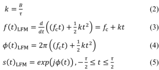
For determining LFM waveform, the design parameters are bandwidth, pulse duration and frequency center. A constant factor, instantaneous phases, instantaneous frequency and LFM waveforms can be calculated respectively in (2) until (5) [6]:
(2)
(3)
2 (4)
, (5)
where is frequency carrier (Hz), B is bandwidth (Hz), τ is pulse duration (second), k is constant factor and t is time (second).
B. Non Linear Frequency Modulation (NLFM)
NLFM waveform has several advantages over LFM. It requires no frequency domain weighting for time sidelobe reduction because the FM modulation of the waveform is designed to provide the desired spectrum shape that yields the required time sidelobelevel [1]. The concept of NLFM waveforms in pulse compression was introduced in the early 1960s and then later became widely used in the 1990s [12]. The most popular method was developed by De Witte and Griffi in 2004 [13]. NLFM has a varied frequency deviation function so the relationship between frequency and time of the signal becomes nonlinear. Effectively, in NLFM, the rate of change of the LFM waveform phase is varied so that less time is spent on the edges of the bandwidth, as illustrated in Figure 3 [10]. This is to reduce high peak sidelobe, so that NLFM method has SNR value and better resolution performance than LFM method.
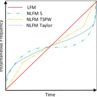
The types of NLFM waveform studied in this paper are NLFM TSPW, NLFMS and NLFM Taylor. NLFM TSPW is a class of frequency modulated pulse compression technique in which sweep rate is not restricted to a constant as compared to the LFM. NLFM TSPW is combination of LFM signals with distinct sweep rates. The frequency of each stage is swept linearly through the given time frame. TSPW linear frequency modulation is carried out in three stages. The chirps design of LFM, NLFM S, TSPW and Taylor can be seen in the Figure 4. The equations of NLFM TSPW can be seen in (6) - (8) [14].
Figure 3. An illustration showing frequency versus time for an LFM waveform (solid line) and a NLFM (dashed line) Figure 2. Chirp waves on LFM; Up-chirp (left); Down-chirp
(right)
Time
In
st
a
n
ta
n
eous
F
re
q
ue
nc
y
NLFM Taylor NLFM TSPW NLFM S LFM
Figure 4. The design of chirp pulse diagram for LFM and NLFM.
,
, ,
(6)
2 ,
2 ,
2 ,
(7)
, (8)
In (6) and (7), B is signal bandwidth (Hz), τ is pulse duration (s), t is time duration (s), B0 is bandwidth 0
(Hz), B1 is bandwidth 1 (Hz), B2 is bandwidth 2 (Hz), T0
is time 0 (second), T1 is time 1 (second), T2 is time 2
(second), is the instantaneous frequency of TSPW and is the instantaneous phase of TSPW. In (8), is the complex signal of TSPW. The equation NLFM S of instantaneous frequency, instantaneous phases and real signal can be seen in (9). Figure 4 shows the chirp of NLFM S. The design of a chirp of NLFM S is built from the formula of tangent function [15].
, 0 ∞ (9)
In (9), α is sidelobecontrol factor of NLFM S.
, (10)
In (10), is instantaneous frequency of NLFMS (Hz), τ is pulse duration (s), B is signal bandwidth (Hz), t is time duration (s) and is frequency center (Hz).
2 , (11)
, (12)
In (11) and (12), is the instantaneous phase of NLFM S and is the complex signal of NLFM S.
TABLE 1
NLFM TAYLOR COEEFICIENTS
n Kn n Kn n Kn
1 -0.114176077 11 -0.001699027 21 -0.000302252 2 0.039601383 12 0.001391083 22 0.000254357 3 -0.020485496 13 -0.001156893 23 -0.000231254 4 0.012533073 14 0.00096693 24 0.000222144 5 -0.008409924 15 -0.000802412 25 -0.000194994 6 0.005986208 16 0.000664113 26 0.000157468 7 -0.004444062 17 -0.000564099 27 -0.000115712 8 0.003400665 18 0.000499719 28 0.000105802 9 -0.002658061 19 -0.000436639 29 -0.000115179 10 0.002109386 20 0.000363526 30 0.000112324
NLFM uses Taylor coefficients can reduce the PSL significantly. This paper will use 30 coefficients (Table 1) for sidelobe suppression in the pulse compression process [16]. The chirps design of NLFM Taylor can be seen in the Figure 4 and the equations of NLFM Taylor can be seen in (13) –(15) [17].
∑
, 13
In (13), is instantaneous frequency of NLFM Taylor, is frequency carrier (Hz), B is signal bandwidth (Hz), τ is pulse duration (s), n is number of Taylor coefficient and is Taylor coefficient.
∑
, (14)
s t exp jϕ t , t (15)
In (14) and (15), is instantaneous phase of NLFM Taylor and is the complex signal of NLFM Taylor.
C. Digital Matched Filtering
Digital matched filtering is a widely used in radar systems because it can increase the signal to noise ratio (SNR). The convolution sum can be implemented in a digital domain, as seen in Figure 5. The computational cost of a digital matched filtering depends on the number of samples N in the pulse duration. Mathematical calculations of digital matched filtering can be seen in (16). x[k] is the received signal sample, and h[k] is the coefficient of the digital filter, where if h[k] = x[k] is the filter corresponding to the transmitted pulse.
∑ ∗ (16)
III. SIMULATION SETUP
A. Pulse Compression Performance
The simulation is conducted to analyze the characteristic of NLFM waveform i.e. NLFM TSPW, NLFM Sand NLFM Taylor. Sidelobe control factor is parameter that is changed to find out the characteristics of each waveform design. The measurement of peak sidelobe level is related to the performance of detectability and width of mainlobe related to the performance of resolution.
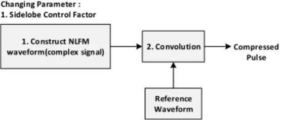
Figure 6 presents the flow of simulation system to evaluate the performance of pulse compression. The first process of the simulation is to generate the NLFM complex signal. The second process is compressing the pulse signal. The last one is to measure the peak sidelobe level and width of mainlobe. The requirements of simulation system of pulse compression performance are:
1. fc: 0 MHz 2. B: 100 MHz 3. fs: 1000Msps 4. τ: 100µs
5. Sidelobe Control Factor (SLCF):
- NLFM TSPW: 0.1 - 0.195
- NLFM S: 1 - 2.45
- NLFM Taylor: 1 – 30
B. Background Noise Effect
Noise can’t be avoided in the radar systems. Additive White Gaussian Noise (AWGN) noise is the natural noise that is always present in every device. AWGN has additive, white, and Gaussian properties, additive properties mean that noise is added to signal, white means that noise is independent of operating system frequency and has constant power density, and Gaussian properties means that the noise voltage has Gaussian distribution. Simulation system of background noise is done by adding AWGN noise before pulse compression process.
2. Convolution
Reference Waveform
Compressed Pulse 1. Construct NLFM
waveform(complex signal) Changing Parameter : 1. Sidelobe Control Factor
Figure 6. Simulation system of pulse compression performance
3. Convolution Compressed Pulse 1. Construct NLFM
waveform(complex signal)
Changing Parameter : 1. SNR(Signal to Noise Ratio)
2. AWGN Changing Parameter :
1. Setting in the lowest PSL 2. Number of Trial
Reference Waveform
Figure 7. Simulation system of background noise effect
Figure 7 shows a simulation system of background noise effect. The first process is to generate the NLFM complex signal with the smallest peak sidelobe level condition. This condition can get from the first simulation result that is simulation system of pulse compression. The second process is generating AWGN noise, and it is added at NLFM complex signal. The third is convolution process. The changing of SNR is done to evaluate the characteristic of the NLFM signal against AWGN noise with trial 200 times. The measurement is done on peak sidelobe level and width of mainlobe. The requirements of simulation system of background noise are:
1. fc: 0 MHz 2. B: 100 MHz 3. fs: 1000 Msps 4. τ: 100µs
5. Number of trial: 200x
6. SLCF: Setting in the lowest PSL
7. SNR: 20 dB, 10 dB, 0 dB, -10 dBand -20 dB
C. Doppler Effect
A radar observing a moving object or target will be cause a Doppler effect and time dilation that will affect the performance of the pulse compression [18] - [19]. The LFM signal has Doppler tolerance when the target conditions at very high speeds but have the same pulse compression performance as the stationary condition. The changing of speed of the target will cause the Doppler frequency and time dilation where with this condition the performance of pulse compression would be measured. Doppler effect measurements were performed on the waveform design of NLFM TSPW, NLFMS and NLFM Taylor.
Figure 8 shows the flow of the simulation system to evaluate the Doppler effect of the compressed signal. The first and second process of the simulation is to generate the NLFM complex signal that has been added with the factor of Doppler frequency and time dilation. The third process is to separate the complex signal into a real signal and an imaginary signal. The fourth process is to generate the NLFM complex signal. The fifth process is to separate the complex signal into the real signal and the imaginary signal. The sixth and seventh process is to convolution process on the signal that has added Doppler effect and time dilation with the original signal. The measurement is done on peak sidelobe level and width of mainlobe.
3. Convolution
Reference Waveform
Compressed Pulse 1. Construct NLFM
waveform(complex signal)+frekuensi doppler Changing Parameter : 1. Doppler Frequency 2. Speed of Target 3. Time Dilation
SNR = ‐ 10dB
2. AWGN
The requirements of simulation system of Doppler Effect are:
1. fc: 0 MHz 2. B: 100 MHz 3. fs: 1000 Msps 4. τ: 100µs
5. Doppler frequency: 0 - 5000 Hz 6. Velocity: 0 -5400 km/hour 7. SLCF: Setting in the lowest PSL 8. SNR: -10 dB
D. Model for Realistic Applications
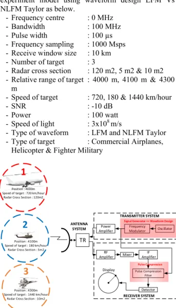
The model for realistic applications was performed by comparing the detection and resolution performance of LFM and NLFM Taylor on radar surveillance as in Figure 9.The experimental model was conduct on the 3 condition of targets where the distance between each targets was very close, the first target was a commercial flying nurse having a RCS of 120 m2 located at a
distance of 4000 meters at a speed of 720 km / hour, the second target was a helicopter having RCS 5m2 at a
distance 4100 meters with a speed of 180 km / hour and the last is a fighter military has RCS 10 m2 is at a
distance of 4300 meters with a speed of 1440 km / hour. Detailed requirements for the radar surveillance experiment model using waveform design LFM Vs NLFM Taylor as below.
- Frequency centre : 0 MHz
- Bandwidth : 100 MHz
- Pulse width : 100 µs
- Frequency sampling : 1000 Msps - Receive window size : 10 km - Number of target : 3
- Radar cross section : 120 m2, 5 m2 & 10 m2 - Relative range of target : 4000 m, 4100 m & 4300
m
- Speed of target : 720, 180 & 1440 km/hour
- SNR : -10 dB
- Power : 100 watt
- Speed of light : 3x10⁸ m/s
- Type of waveform : LFM and NLFM Taylor - Type of target : Commercial Airplanes,
Helicopter & Fighter Military
TR
Power
Amplifier Oscillator
Frequency Modulator
RF
Amplifier Mixer
IF Amplifier
Pulse Compression Filter
Detector
Display
TRANSMITTER SYSTEM
RECEIVER SYSTEM ANTENNA
SYSTEM
Signal Generator == Waveform Design
Pulse Compression
Position : 4000m Speed of target : 720 km/hour
Radar Cross Section : 120m2
Position : 4100m Speed of target : 180 km/hour
Radar Cross Section : 5m2
Position : 4300m Speed of target : 1440 km/hour
Radar Cross Section : 10m2
1
2
3
Figure 9. Block diagram of experiments model for surveillance radar
(17)
In (17), is time of target (seconds), is distance of target (meter), is speed of target (m/s), is time (seconds), is speed of light (3x10⁸m/s).
(18)
In (18), ′ is time dilation (seconds) and is pulse width (seconds)
(19)
In (19), is doppler frequency (Hz) and : wavelength (meter).
The equations of LFM original signal can be seen in (2) until (5). Substituting is done between (2) and (18) and then between (4) with (17), (18) and (19) where the result of substituting is at (20) – (22). Equations (20) until (22) are formula of LFM to calculate the signal echo from target reflection.
(20)
2 (21)
, (22)
The equations of NLFM Taylor original signal can be seen in (13) until (15). Substituting is done between (14) and (17), (18) and (19) where the result of substituting is at the below equations. Equations (23) until (26) are formula of NLFM Taylor to calculate the signal echo from target reflection.
(23)
∑ (24)
(25)
, (26)
IV. RESULTS AND DISCUSSION
A. Analysis of Pulse Compression Performance
From Figure 10, increasing the SLCF of NLFM, it will decrease the peak sidelobe level and increase the resolution performance of radar. The maximum PSL of NLFM that can be suppressed about -20.88 dB (TSPW), -29.83 dB(S) and -38.86 dB(Taylor). NLFM Taylor is the most powerful for suppressing PSL when enhance the SLCF than NLFM TSPW and NLFM S.
From Figure 11, the width of mainlobe of NLFM TSPW and Taylor is not influence when changes occur for SLCF values, the width of mainlobe is stable at 0.0121 µs for TSPW and around 0.0172 µs until 0.0174 µs for taylor. But the width of mainlobeof NLFM S has most affected when increasing the value of SLCF, it’s from 0.0121µs until 0.0181µs.
From Figure 12, it’s the matched filter output for NLFM TSPW, S and Taylor. The best pulse compression is NLFM Taylor because can suppress PSL up to -38 dB with 30 coefficients while NLFM S can suppress PSL up to -22 dB and NLFM TPSW can suppress PSL up to -20 dB.
Figure 10. Peak Sidelobe Level of NLFM TSPW, S & Taylor
Figure 11. Width of mainlobe of NLFM TSPW, S & Taylor
Figure 12. Matched filter output of NLFM TSPW, S & Taylor
Figure 13. Background noise to PSL of NLFM TSPW, S & Taylor
B. Analysis of Background Noise Effect
The background noise effect analysis is performed to analyze the effect on pulse compression performance on waveform design of NLFM. The simulation is done by adding AWGN noise on complex NLFM signal with SNR 20 dB up to -20 dB where the measurement is by doing trial 200 times and taking the mean value. Measurements and analysis were performed on peak sidelobe level and width of mainlobe.
The decreased of signal to noise ratio causes the peak sidelobe level increase. Vice versa, the increasing of signal to noise ratio would be effect to the value of peak sidelobe level(PSL) smaller. From Figure 13, at SNR 20 dB, the PSL value of NLFM Taylor is around -38.71 dB and when SNR drops to -20 dB, peak sidelobe level rises to around -18.29 dB, whereas in NLFM S when SNR is 20 dB, peak sidelobe level is around -31.59 dB and when the SNR drops -20 dB, the peak sidelobe level becomes around -18.16dB. From Figure 14 the SNR changes from -20 dB to 20 dB did not significantly affect to the Width of Mainlobe (WoM).
C. Analysis of Doppler Effect
To evaluate the Doppler effect of the NLFM waveforms, there are several parameters that will be analyzed, such as peak sidelobe level and mainlobe level (MLL).The factors that would affect in Doppler effect are Doppler frequency and time dilation that influenced by speed of the target or object. This simulation is performed to compare the characteristic of some NLFM waveforms against Doppler effect with frequency of radar in 500 MHz and speed of the target from 0 km/hour until 5400 km/hour.
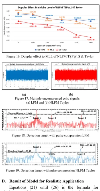
From Figure 15, the Doppler effect is to enhance the peak sidelobe level (PSL). NLFM Taylor is the most effected by Doppler frequency but it has the lowest of PSL. In the stationary condition the PSL of NLFM Taylor is around -38.86 dB, when the target has speed with 1080 km/hour the value of PSL become around -33.33 dB. From Figure 16, the speed of the target increases, the mainlobe level would be decreased.
Figure 14. Background noiseto WoM of NLFM TSPW, S & Taylor
Figure 16. Doppler effect to MLL of NLFM TSPW, S & Taylor
D. Result of Model for Realistic Application
Equations (21) until (26) is the formula for obtaining multiple uncompressed echo signals based on the requirements of Figure 9 where simulations are performed on three targets with different RCS parameters and with adjacent spacing. The simulation result of multiple uncompressed echo signals LFM and NLFM Taylor can be seen in Figure 17, the simulation is done on signal to noise ratio of 0 dB.
Figure 18 depicts the result of the pulse compression and detection target of the experiment model in Figure 9. In Figure 18, by using LFM method produces a high of peak sidelobe level about -13.24dB at target 1 while the signal level at target 2 is about -14.71 dB and at target 3 around -13.29 dB. With a threshold of level -13 dB, target 2 and target 3 will not be detected by the radar because it is considered noise whereas if the threshold level is loweredaround -15 dB, target 2 and target 3 will be detected but the peak sidelobe level on the first target will be detected as target and false detection occurs.
Figure 19 is the result of detection target pulse compression with NLFM Taylor using the number of coefficients 30 where the simulation of peak sidelobe level has a smaller value when compared with LFM. With the threshold level -23 dB, target 1, target 2 and target 3 are detected as targets and no false detection
occurs because the signal level of the target is greater than the threshold level.
V. CONCLUSIONS
Waveform Design of NLFM TSPW, NLFM S and NLFM Taylor can be suppressed the peak sidelobe level better than the conventional LFM. NLFM TSPW can suppress the peak sidelobe level up to -21 dB, NLFM S can suppress the peak sidelobe level-up to -29 dB and NLFM Taylor can suppress peak sidelobe levelup to -38dB but the impact is the width of mainlobe become bigger so that pulse compression ratio parameter is smaller.
The lower SNR value causes the peak sidelobe parameter level to decrease, while the mainlobe level and width of mainlobe parameters are not too affected by SNR changes in conditions 20 dB up to -20dB. When the target moves will cause Doppler effect and time dilation.Therefore, as the target moves from stationary to high-speed conditions the parameters of the peak sidelobe level increase linearly as the speed of target increases, while the values of mainlobe parameters tend to decrease while the mainlobe level and width of mainlobe parameters are not too affected by moving of the target.
The method of NLFM is better than LFM for detectability and resolution in the applications for radar surveillance because NLFM can suppress the PSL and then the level of the threshold become decrease.
REFERENCES
[1] M. I. Skolnik, Radar Handbook, 3rd ed. New York: McGraw-Hill, 2008.
[2] A. K. Sahoo, “Development of radar pulse compression techniques using computational intelligence tools,” Ph.D. dissertation, Institute of Technology Rourkela, 2012.
[3] C. Kumar, “Development of efficient radar pulse compression technique for frequency modulated pulses,” M.S. thesis, Institute of Technology, Rourkela, 2014.
[4] M. I. Skolnik, Introduction to Radar System, 2nd ed. McGraw-Hill, 1981.
[5] I. Intyas, R. Hasanah, M. R. Hidayat, B. Hasanah, A. B. Suskmono, A. Munir, “Improvement of radar performance using LFM pulse compression technique,” in 2015 Int. Conf. Elect.
Eng. Informatics (ICEEI), Bali, Indonesia, 2015.
[6] B. P. A. Rohman, R. Indrawijaya, D. Kurniawan, O. Heriana, C. B. A. Wael, “Sidelobe suppression on pulse compression using curve-shaped nonlinear frequency modulation,” in 2016 1st Int.
Conf. Inform. Technology, Inform. Syst. Elect. Eng. (ICITISEE),
Yogyakarta, Indonesia, 2016.
[7] S. Boukeffa, Y. Jiang, T. Jiang. “Sidelobe reduction with nonlinear frequency modulated waveforms,” in 2011 IEEE 7th
Int. Colloq. Signal Process. and its Applicat. (CSPA), Penang,
Malaysia, 2011.
[8] A. W. Doerry, “Generating nonlinear FM chirp waveforms for radar,” Sandia National Laboratories, California, 2006. [9] S. Parwana, S. Kumar, “Analysis of LFM and NLFM radar
waveforms and their performance analysis,” Int. Res. J. Eng. Tech., 2015.
[10] B. R. Mahafza, Radar Systems Analysis and Design Using
MATLAB, 3rd ed. Florida: CRC Press, 2013.
[11] A. Orduyılmaz, G. Kara, M. Serin, A. Yıldırım, A. C. Gürbüz, M. Efe, “Real-time pulse compression radar waveform generation and digital matched filtering,” in 2015 IEEE Radar
Conf. (RadarCon), USA, 2015.
[12] H. D. Griffiths and L. Vinagre, “Design of low-sidelobe pulse compression waveforms,” Electron. Lett., vol. 30, no. 12, Jun. 1994.
8
Figure 19. Detection target withpulse compression NLFM Taylor Figure 18. Detection target with pulse compression LFM
(a) (b) Figure 17. Multiple uncompressed echo signals,
(a) LFM and (b) NLFM Taylor
[13] E. D. Witte and H. D. Griffiths, ”Improved ultra-low range sidelobe pulse compression waveform design,” Electron. Lett., vol. 40, no. 22, Oct. 2004.
[14] R. Jeevanmai and N. D. Rani, “Sidelobe reduction using frequency modulated pulse compression techniques in radar,”
Int. J. Latest Trends Eng. Tech., vol. 7, no. 3, pp.171-179, 2013.
[15] J. Song, Y. Gao, and D. Gao, “Analysis and detection of S-shaped NLFM signal based on instantaneous frequency,” J.
Commun., vol. 10, no. 12, Dec. 2015.
[16] L. R. Varshney and D. Thomas, “Sidelobe reduction for matched filter range processing,” in the 2003 IEEE Radar Conf., USA, 2003.
[17] I. C. Vizitiu, F. Enache and F. Popescu, “Sidelobe reduction in pulse-compression radar using the stationary phase technique: an extended comparative study,” in 2014 Int. Conf. Optimization
Electr. Electron. Equipment (OPTIM), Romania, 2014.
[18] B. P. A. Rohman, et al., “Performance analysis of curve-shaped NLFM against doppler effect and background noise,” in 2016 Int. Conf. Radar Antenna Microw. Electron.
Telecommunications (ICRAMET), Indonesia, 2016.
[19] T. Collins and P. Atkins, “Nonlinear frequency modulation chirps for active sonar,” in IEE Proc. Radar Sonar