Article
Population differentiation at a regional scale in
spadefoot toads: contributions of distance and
divergent selective environments
Amber M. R
ICE*, Michael A. M
CQ
UILLAN, Heidi A. S
EEARS, and
Joanna A. W
ARRENDepartment of Biological Sciences, Lehigh University, Bethlehem, PA 18015, USA
*Address correspondence to Amber M. Rice. E-mail: [email protected].
H.A. Seears is now at the Department of Biology, University of Virginia, Charlottesville, VA 22904, USA
J.A. Warren is now at the Department of Microbiology and Immunology, University of North Carolina, Chapel Hill, NC 27599, USA
Received on 2 September 2015; accepted on 16 January 2016
Abstract
The causes of population differentiation can provide insight into the origins of early barriers to gene
flow. Two key drivers of population differentiation are geographic distance and local adaptation to
di-vergent selective environments. When reproductive isolation arises because some populations of a
species are under selection to avoid hybridization while others are not, population differentiation and
even speciation can result. Spadefoot toad populations
Spea multiplicata
that are sympatric with a
con-gener have undergone reinforcement. This reinforcement has resulted not only in increased
reproduct-ive isolation from the congener, but also in the evolution of reproductreproduct-ive isolation from nearby and
dis-tant conspecific allopatric populations. We used multiple approaches to evaluate the contributions of
geographic distance and divergent selective environments to population structure across this regional
scale in
S. multiplicata
, based on genotypes from six nuclear microsatellite markers. We compared
groups of populations varying in both geographic location and in the presence of a congener.
Hierarchical F-statistics and results from cluster analyses and discriminant analyses of principal
com-ponents all indicate that geographic distance is the stronger contributor to genetic differentiation
among
S. multiplicata
populations at a regional scale. However, we found evidence that adaptation to
divergent selective environments also contributes to population structure. Our findings highlight how
variation in the balance of evolutionary forces acting across a species’ range can lead to variation in
the relative contributions of geographic distance and local adaptation to population differentiation
across different spatial scales.
Key words: cascade reinforcement, character displacement, reproductive isolation, spatial scale,Spea multiplicata, speciation.
Elucidating the causes of genetic differentiation between popula-tions of a single species can provide important insight into the speci-ation process, because the origins of early barriers to gene flow may often be concealed by evolutionary divergence after speciation (Via 2009). Even though incompletely isolated populations may not all proceed to complete reproductive isolation and species status (Nosil et al. 2009b), the mechanisms underlying population differentiation
are key for explaining biological diversity. Further, understanding the relative contributions of geographic distance and divergent selec-tion, two potential factors underlying genetic differentiaselec-tion, can shed light on longstanding questions about the importance of gen-etic drift versus selection in speciation (Coyne and Orr 2004).
Local adaptation is an important driver of population differenti-ation and specidifferenti-ation (Shafer and Wolf 2013;Sexton et al. 2014). When
VCThe Author (2016). Published by Oxford University Press. 193
This is an Open Access article distributed under the terms of the Creative Commons Attribution Non-Commercial License (http://creativecommons.org/licenses/by-nc/4.0/), which permits non-commercial re-use, distribution, and reproduction in any medium, provided the original work is properly cited. For commercial re-use, please contact [email protected]
populations adapt to different environments, gene flow between them may be reduced for multiple reasons (Schluter 2001;Rundle and Nosil 2005). When migrants mate with residents, any offspring that are phenotypically intermediate or otherwise mismatched to the environ-ment are likely to be selected against, resulting in extrinsic postzygotic reproductive isolation (Hatfield and Schluter 1999;Pfennig and Rice 2007;Fuller 2008;Arnegard et al. 2014). Local adaptation may also reduce the likelihood of such matings. If migrants from alternate envir-onments are maladapted to local conditions, they are less likely to sur-vive to successfully reproduce (“immigrant inviability,”sensu Nosil et al. 2005). Likewise, when local adaptation results in the divergence of sexual signals or mating preferences, premating isolation can arise (Jiggins et al. 2004;Snowberg and Benkman 2007;Pfennig and Rice 2014).
Such mating trait divergence can not only arise when populations adapt to divergent ecological environments, but also when populations vary in the presence of an interacting species (Hoskin and Higgie 2010;Pfennig and Rice 2014). For instance, when some populations of a species co-occur with a closely related species while other popula-tions do not (i.e., sympatric and allopatric populapopula-tions, respectively), selection will act differently in these two environments. As a result of selection to avoid interspecific mating interactions or hybridization, sympatric populations might undergo reproductive character displace-ment (RCD) or reinforcedisplace-ment (Pfennig and Pfennig 2012); allopatric populations, on the other hand, do not. When the resulting divergence in mating traits between allopatric and sympatric populations results in reproductive isolation, speciation can occur. This process has been called both “RCD speciation” (Hoskin and Higgie 2010) and “cas-cade reinforcement” (Ortiz-Barrientos et al. 2009), and recent empir-ical and theoretempir-ical results suggest it may be an important initiator of speciation (Hoskin et al. 2005; Jaenike et al. 2006; McPeek and Gavrilets 2006, Pfennig and Ryan 2006, Svensson et al. 2006,
Lemmon 2009,Porretta and Urbanelli 2012;Bewick and Dyer 2014;
Pfennig and Rice 2014).
The reduction in gene flow because of adaptation to divergent se-lective environments has been called both “isolation by ecology” (IBE;Edelaar et al. 2012) and “isolation by adaptation” (IBA;Nosil et al. 2008). Yet, although IBE is an important and widespread pat-tern of gene flow (Shafer and Wolf 2013;Sexton et al. 2014), levels of gene flow are often affected by geographic distance as well (“‘iso-lation by distance” or IBD;Wright 1943). If dispersal is limited, then the likelihood of mating should be inversely related to the geo-graphic distance separating individuals. In such a scenario, genetic drift alone can lead to population genetic differentiation. Understanding the relative contributions of divergent selective envir-onments and geographic distance to population differentiation is further complicated by the fact that the two factors are often con-founded; populations separated by large distances are more likely to experience different selective environments than are populations separated by small distances. Further, the relative roles of contribu-tors to population structure may fluctuate across the landscape, due to variation in demographic parameters, the strength of divergent se-lection, or other factors.
Here, we examine the relative contributions of geographic distance and divergent selective environments to population differentiation at a regional scale in a system that exhibits both limited dispersal and reinforcement—the spadefoot toadSpea multiplicata. Premating isola-tion is present in this species between populaisola-tions that have and have not undergone reinforcement, at both local and regional scales (Pfennig 2000; Pfennig and Rice 2014). At the local scale, population
differentiation is associated with this difference in selective environ-ment (Rice and Pfennig 2010; Pfennig and Rice 2014); however, whether divergent selective environments contribute strongly to popu-lation structure at the regional scale remains unknown. To address this topic, we used multiple approaches to estimate population struc-ture between groups of populations that varied in both selective envir-onment and geographic location.
Materials and Methods
Study system
The overall goal of this study was to evaluate the contributions of geographic distance and divergent selective environments to popula-tion differentiapopula-tion at a regional scale in the spadefoot toadSpea multiplicata. This species ranges from the southwestern United States into Mexico (Stebbins 2003). In the southwestern United States,S. multiplicata’s range overlaps broadly with the range of a congener,S. bombifrons(Stebbins 2003). During much of the year, individuals hibernate underground, emerging only during the sum-mer months to breed and to feed (Bragg 1944,1945). These species are explosive breeders in ephemeral ponds, formed during the sum-mer rainy season (Bragg 1945). Where the ranges of the two species overlap, ponds vary locally in species composition: Some ponds con-tain only one species, while others concon-tain both (Pfennig and Murphy 2000,2002).
In ponds where the two species co-occur, they occasionally hy-bridize (Simovich and Sassaman 1986;Pfennig and Simovich 2002;
Pfennig et al. 2012). This hybridization is costly forS. bombifronsin certain environments and always costly forS. multiplicata(Pfennig and Simovich 2002). As an indirect effect of selection against hy-bridization in sympatry, femaleS. multiplicatain sympatry versus allopatry withS. bombifronsexperience divergent selective pressure on mate preferences. AllopatricS. multiplicatafemales can obtain fitness benefits by choosing males with faster calls (Pfennig 2000). In contrast, because the fast calls ofS. multiplicataare similar to the calls of S. bombifrons males, sympatric S. multiplicata females lessen their risk of hybridizing by preferring males with slower call rates (Pfennig 2000). Consistent with the occurrence of reinforce-ment in sympatric populations, hybridization frequency has declined over time (Pfennig 2003). As a result of this divergent selection on female preferences between sympatric and allopatricS. multiplicata, premating reproductive isolation has evolved at both local (Pfennig and Rice 2014) and regional scales (Pfennig 2000): Females from both distant and nearby allopatric ponds prefer the calls of males from their own environments over the calls of males from sympatric ponds, and vice versa. Reinforcement has therefore led indirectly to the evolution of reproductive isolation in this species.
As a result of the reproductive isolation that has evolved between S. multiplicatapopulations in sympatry and allopatry withS. bombi-frons, populations from the different selective environments should show signs of differentiation, relative to populations from the same se-lective environment. This prediction has been supported at a local scale by population genetic analyses of southeastern Arizona sympat-ric and allopatsympat-ric populations (i.e., “East” populations, Figure 1,
the extent of population differentiation between populations at this larger scale, and the relative contributions of divergent selection versus geographic distance, remain unknown.
Sampling and genotyping
We analyzed genetic differentiation among 13 populations ofS. mul-tiplicata(Figure 1,Table 1) at 6 previously published microsatellite loci: Sb8 (Pfennig & Rice 2014), Spea C7, Spea D111, Spea D103 (Van Den Bussche et al. 2009), Sm14, and Sm25 (Rice et al. 2008). Each population was categorized based on its relative geographical lo-cation (Table 1, Figure 1; West, Central, or East) and its selective
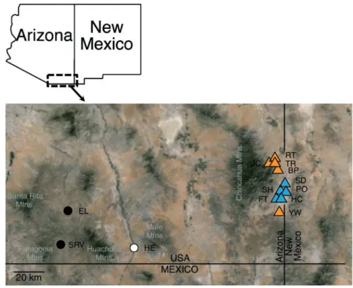
environment (Table 1,Figure 1; Sympatry¼S. bombifronspresent, Allopatry¼ S. bombifrons absent). Genotypes from 11 of the 13 populations were generated for another study (Pfennig and Rice 2014; Table 1) and were reanalyzed for this study. We extracted DNA fromS. multiplicatatissues that were collected from two add-itional populations located at least 65 km west of theS. bombifrons range edge (Figure 1;Table 1; tissues collected by K. and D. Pfennig). The DNA was extracted using a Qiagen (Valencia, California, USA) DNeasy Blood & Tissue Kit, following the manufacturer’s instruc-tions. We used a three-primer system to amplify the microsatellite markers, followingPfennig & Rice (2014). Sample sizes ranged from 10 to 25 per population (Table 1), similar to or greater than sample Figure 1.Map ofSpea multiplicatapopulation locations. Inset at upper left indicates map region. Black circles, west allopatric populations; white circle, central/ west allopatric population; triangles, east populations. Triangle color indicates selective environment, with blue triangles as allopatric, and orange triangles as sympatric. Populations labeled followingTable 1.
Table 1. Sampling and location information
Population code N UTM Northing (m) UTM Easting (m) Geographical category Selective environment category
FT 12 3,513,168.81 680,005.47 East Sympatry
SD 16 3,521,287.58 684,419.76 East Sympatry
BP 18 3,529,290.03 679,851.46 East Allopatry
HC 10 3,513,359.11 680,335.65 East Sympatry
JC 10 3,534,202.38 676,772.4 East Allopatry
PO 13 3,515,338.54 682,464.08 East Sympatry
RT 19 3,535,263.87 677,991.59 East Allopatry
SH 11 3,516,255.27 681,712.24 East Sympatry
TR 10 3,534,235.32 677,745.99 East Allopatry
YW 19 3,502,192.61 680,817.35 East Allopatry
SRV 16 3,475,853.35 538,989.31 West Allopatry
ELa 25 3,501,820.85 541,362.27 West Allopatry
HEa 25 3,477,602.55 585,843.69 Central/Westb Allopatry
aNew genotypic data presented in this study. Genotypes from the other eleven populations were previously generated forPfennig and Rice (2014)and re-analyzed
for this study.
sizes used in previous studies of population structure in this system (Rice and Pfennig 2008, 2010;Pfennig and Rice 2014;Rice et al. 2009). Although small sample sizes per population can decrease abil-ity to accurately estimate allele frequencies, they are still useful for measuring genetic distance (Kalinowski 2005; Pruett and Winker 2008). Our choice to sample more populations over increasing sample sizes per population maximized our power to detect structure be-tween groups of populations (Fitzpatrick 2009). Additionally, all of the genotypes from populations in sympatry withS. bombifronswere previously verified to be from pure-speciesS. multiplicata(Pfennig and Rice 2014). Thus, population differentiation cannot be explained by introgression withS. bombifrons.
Analyses
We used probability tests in Genepop 4.2 (Raymond and Rousset 1995;Rousset 2008) as implemented by Genepop on the Web (http:// genepop.curtin.edu.au), to test for Hardy Weinberg Equilibrium and for genotypic linkage disequilibrium between all locus pairs across all populations. We also ran global tests for Hardy Weinberg for each locus across all populations using Fisher’s method. The default Markov chain parameters were used for both linkage disequilibrium and Hardy Weinberg Equilibrium tests (i.e., 1,000 step dememoriza-tion, 100 batches, and 1,000 iterations per batch). Because only one locus was in Hardy Weinberg Equilibrium (see Results), we used Micro-Checker (van Oosterhout et al. 2004) to test whether the devi-ations from Hardy Weinberg were consistent with the presence of null alleles, using 1,000 randomizations and Bonferroni correction for multiple testing. Null alleles can affect estimates of population structure (Chapuis and Estoup 2006;Carlsson 2008; Guillot et al. 2008), so the Oosterhout correction algorithm was implemented in Micro-Checker (van Oosterhout et al. 2004) to estimate null allele frequencies and to generate corrected allele frequencies and genotypes for use in subsequent analyses where possible (see below).
We used several approaches to test for contributions of geographic distance and divergent selective environments on conspecific popula-tion differentiapopula-tion inS. multiplicata. First, we assigned the populations to groups based on either geography or selective environment (Figure 1;Table 1). If geographic distance contributes more to the observed population differentiation than divergent selective environments, then the geographic population grouping should explain a greater propor-tion of the variapropor-tion in genotype frequencies than the selective environ-ment grouping. If the different selective environenviron-ments make a greater contribution to population differentiation, however, then the opposite should be true.
To do this, we first used Analyses of Molecular Variance (AMOVA) in Arlequin 3.5 (Excoffier and Lischer 2010) to estimate population structure for our entire dataset. The 13 populations were grouped in three ways (Figure 1;Table 1), and hierarchicalF -statis-tics were calculated to test which grouping explained the greatest percentage of variation in microsatellite genotypes (Crispo et al. 2006). We calculatedFSTand otherF-statistics throughout instead ofRSTbecause simulations have shown thatFSToutperformsRSTin conditions of moderate to small sample sizes and numbers of loci (Gaggiotti et al. 1999). The populations were placed either in three geographic groups (i.e., West, Central, East), in two geographic groups (i.e., West, East), or in two selective environment groups (i.e., Sympatric, Allopatric). In each of these cases, we calculated globalFSTandFCTas weighted averages across loci.FSTvalues indi-cate the proportion of the total variation in allele frequency that is explained by variation among the 13 populations, whileFCTvalues
indicate the proportion of the total variation in allele frequency that is explained by the geographic or selective groupings. We also calcu-lated the sameF-statistics for each locus individually. Because null alleles were likely present in our data (see “Results” section), we cal-culatedFSTandFCTfor each locus a second time using corrected al-lele frequencies. GlobalF-statistics were not calculated for the null allele-corrected data because corrected data could only be input in a format that does not allow multi-locus analyses in Arlequin. Significance of theF-statistics was estimated using 10,000 permuta-tions of the data.
We next used the adegenet package (Jombart 2008;Jombart and Ahmed 2011) in R version 3.2.1 (R Core Team 2015) to assess the genetic population structure present among our different population groupings using Discriminant Analyses of Principal Components (DAPC) (Jombart et al. 2010). DAPC does not rely on assumptions of Hardy Weinberg Equilibrium (Jombart et al. 2010). It first trans-forms multi-locus genetic data into a set of fewer, uncorrelated vari-ables using a principal components analysis; a discriminant analysis is then applied to a set of retained principal components, such that the variation between defined groups is maximized. In addition to allowing graphical assessment of population structure, DAPC also calculates the proportion of successful reassignment of individuals to their previously defined groups, based on the discriminant func-tions. A high proportion of successful reassignment indicates that the groups are genetically distinct, while a lower proportion suggests little structure between the groups. To test for contributions of geo-graphic distance and selective environment on population structure inS. multiplicata, we performed DAPC analyses using the three pre-viously described population groupings. If geographic distance con-tributes more than divergent selective environments to population structure inS. multiplicata, then we expected higher proportions of successful reassignment to geographic groups than to selective envir-onment groups. Alternatively, if divergent selective envirenvir-onments contribute more, then higher proportions of successful reassignment to selective environment groups were expected. Because retaining too many principal components can lead to inflated reassignment success, we followed the recommendations of the DAPC tutorial and performed an a-score optimization to determine the optimal number of principal components to retain for each DAPC analysis. We then ran DAPC three times for each population grouping, retain-ing different numbers of principal components: 1) the optimal num-ber based on a-score optimization; 2) the minimum optimal numnum-ber across all groupings (i.e., 7; see “Results” section); and 3) the max-imum optimal number across all groupings (i.e., 41; see “Results” section). Based on our results, we performed an additional DAPC analysis on a combined geographic and selective environment grouping (Figure 1; Table 1; i.e., West/Central allopatry, East allopatry, and Sympatry), and retained only the optimal number of principal components based on a-score optimization.
assuming Hardy Weinberg Equilibrium within populations (Guillot et al. 2005); however, it also incorporates an optional algorithm to improve the accuracy of inferences when null alleles are present (Guillot et al. 2008). To estimate the number of genetic clusters pre-sent in our data, we ran ten independent runs of Geneland under each of two different sets of modeling parameters. Both parameter sets included the spatial model (incorporating 100 m coordinate un-certainty), the null allele filtering algorithm, a maximum of 13 populations, 1,000,000 Markov chain Monte Carlo (MCMC) itera-tions with every 1,000th iteration saved, and 200 saved iterations discarded as burn-in. The spatial coordinates were expressed in the Universal Transverse Mercator (UTM) coordinate system (Table 1). The first parameter set used the uncorrelated allele frequency model, and the second set used the correlated allele frequency model. Even though the correlated allele frequency model is likely to be a more accurate reflection of the biology ofS. multiplicata, and may have more power to detect subtle population differentiation (Guillot 2008), it may also be less robust to deviations from model assump-tions. For this reason, we followed the suggestions of the Geneland manual, and ran both correlated and uncorrelated allele frequency models. We checked that the 10 independent runs under each para-meter set inferred similar numbers of clusters, in order to ensure that we ran Geneland for enough iterations. We then ran longer, single runs of Geneland under each parameter set, with 2,000,000 MCMC iterations, every 1,000thiteration saved, and 400 saved iterations discarded as burn-in, to obtain final estimates of cluster number. We visualized probability of population assignment to genetic clusters using the program distruct 1.1 (Rosenberg 2004).
It is important to note that although the preceding analyses allow us to test predictions about the relative contributions of geographic grouping versus selective environment on population differentiation, they do not allow us to directly compare the relative contributions of these effects in a single analysis. This is unfortunate, because eco-logical differences will often be confounded with geographic dis-tance (Sexton et al. 2014), which is the case in our system (Figure 1). In recent years, a number of approaches have been developed to ad-dress this problem (e.g.,Bradburd et al. 2013;Wang 2013b). Here, we employed three approaches in an effort to address this issue.
First, we performed a two-factor AMOVA to simultaneously es-timate the effects of geography and selective environment on genetic variation. We used the PopGenReport package (Adamack and Gruber 2014) in R version 3.2.2 (R Core Team 2015) to calculate pairwise genetic distances among all individuals, based onKosman and Leonard’s (2005)genetic distance measure. We then used the adonisfunction in the vegan package (Oksanen et al. 2015) to run a two-factor AMOVA. As factors, we used geographic group (two lev-els: West, East) and selective environment (two levlev-els: Sympatric, Allopatric). Significance was estimated withF-tests based on sequen-tial sums of squares, using 1,000 permutations of the raw data.
The two-factor AMOVA tests the explanatory power of categorical variables; therefore, it does not include an explicit test for a linear rela-tionship between geographic and genetic distance. Thus, we also per-formed a multiple matrix regression with randomization (MMRR) in R version 3.2.2 (R Core Team 2015) using the script supplied by Wang (2013a,2013b) to simultaneously estimate the contributions of geo-graphic distance and divergent selective environments to population differentiation. Our response matrix for this analysis was population pairwiseFST, calculated in Arlequin 3.5 (Excoffier and Lischer 2010) without correcting for the presence of null alleles. We included all com-binations of three predictor matrices: 1) a binary selective environment contrast matrix, with 0 representing a comparison between two
populations from the same selective environment, and 1 representing a comparison between two populations from different selective environ-ments; 2) a Euclidean (i.e., straight line) geographic distance matrix, with pairwise distances calculated from the population UTM coordin-ates (Table 1); and 3) an environmental cost distance matrix (following
Wang and Summers 2010). An environmental cost path analysis, also known as least-cost path analysis, determines the length of the most likely dispersal path by weighting potential dispersal paths between populations by predicted climate and elevation requirements for the species.
To calculate the environmental cost distance matrix, we first per-formed species distribution modeling to predict the environmentally suitable range forS. multiplicata. We extracted contemporary cli-mate and elevation data (averages for years 1950–2000) from the WorldClim database (worldclim.org,Hijmans et al. 2005) at 30 arc-second resolution, and cropped the climate and elevation layers to include areas between latitudes 23N–40N and longitudes 96W113W. We used all 19 bioclimatic variables, representing trends in temperature and precipitation, seasonality, and extreme or limiting environmental factors, plus elevation for our species distri-bution modeling. We obtained 268 georeferenced species occurrence locations from across the entire range ofS. multiplicatabased on the samples from this study (Table 1) plus records from 22 museums (data provided by A. Chunco;Chunco et al. 2012). After filtering out any samples occurring in the same grid cell, 236 records were left for building our distribution model. We used MAXENT version 3.3.3k (Phillips et al. 2006) to predict habitat suitability at each grid cell of the study area, with values ranging from 0 (unsuitable habi-tat) to 1 (fully suitable habihabi-tat). We then inverted the suitability val-ues to create friction landscapes (i.e., cost valval-ues), and calculated pairwise environmental cost distances (i.e., least-cost paths) among our 13 populations using SDMtoolbox (Etherington 2011;Brown 2014) in ArcMap (ver. 10.2.2; ESRI, Redlands, CA, USA).
All matrices were standardized by subtracting the matrix mean from each value and dividing by the matrix standard deviation, as recommended in the MMRR tutorial (Wang 2013a).P-values were calculated using 10,000 permutations of the data. The predictor ma-trix with the largest significant regression coefficient contributes the most to population differentiation at this regional scale (Wang 2013b;
Nanninga et al. 2014).
Thirdly, we performed one final DAPC analysis on the subset of in-dividuals within the East geographic group, grouped by selective envir-onment (Figure 1;Table 1). We retained only the optimal number of principal components based on a-score optimization. With this ana-lysis, we examined the assignment of individuals from the YW popula-tion, which experiences an allopatric selective environment (Table 1), but is geographically nearer to the sympatric populations (Figure 1). If selective environment contributes to population structure, then individ-uals from the YW population should be correctly assigned to the allo-patric selective environment grouping; however, if geographic distance is the sole contributor to population structure, then individuals from the YW population should instead be assigned to the sympatric selective environment grouping.
Results
Linkage disequilibrium and Hardy Weinberg
equilibrium
equilibrium (P>0.19). Our six loci therefore provided independent data on population structure, and we retained genotypes from all six loci for subsequent analyses. Of the 78 possible population–locus combinations, five could not be tested for departure from Hardy Weinberg Equilibrium, either because the locus exhibited no poly-morphism in a particular population (three of five cases, all Sb8), or
because the locus failed to amplify in all individuals of a particular population (two of five cases, all SpeaD103). A majority of the re-maining 73 population–locus combinations showed evidence of de-parture from Hardy Weinberg equilibrium atP<0.05 (Table 2). In most cases, the pattern of departure from Hardy Weinberg equilib-rium was consistent with the presence of a null allele (Table 2). Allele frequencies and genotypes corrected for the presence of null alleles using the Oosterhout algorithm in Micro-Checker (van Oosterhout et al. 2004) were therefore used when possible in our analyses of population structure.
Population structure
Results from the AMOVAs comparing different groupings of the full dataset are presented inTable 3.FSTvalues were significantly greater than zero for individual loci and for the global weighted average across loci. Although individual locus FSTvalues tended to decrease after correction for the presence of null alleles, they re-mained significantly greater than zero. Additionally,FSTvalues were universally higher than corresponding FCTvalues. Global weighted averageFCTvalues were significantly greater than zero for two of the population grouping schemes (Table 3), with a higher globalFCT for two geographic groups versus two selective environment groups. This suggests that grouping the populations into two geographic groups explains a higher proportion of the total genotypic variation than does grouping by selective environment. At the individual locus level, only one to three loci exhibited significant FCT values,
Table 2. Summary of tests for Hardy Weinberg Equilibrium and null alleles
Sb8 SpeaC7 SpeaD111 Sm25 Sm14 SpeaD103
FT N/A X X N/A
SD X X X N/A
BP X X X X
HC X X X
JC X X X X
PO X X X X X
RT N/A X
SH X X X X
TR X X X
YW X X X X X
SRV N/A X X
EL X X
HE X X
Gray shading: significant evidence of null allele; X: significant deviation from Hardy Weinberg Equilibrium; N/A: no information because allele is fixed or failed to amplify.
Table 3. AMOVA results comparing different groupings of the full dataset
Sb8 SpeaC7 SpeaD111 Sm25 Sm14 SpeaD103a
Globalb
A. Three geographic groups (West, Central, East)
FST, uncorrected (P-value) 0.13333 (0.000) 0.08004 (0.000) 0.08016 (0.000) 0.10425 (0.000) 0.05578 (0.000) 0.05090 (0.002) 0.08520 (0.000) FST, corrected (P-value) 0.15638 (0.000) 0.04704 (0.004) 0.04671 (0.000) 0.07942 (0.000) 0.01982 (0.013) 0.03702 (0.017)
FCT, uncorrected (P-value) 0.05181 (0.741) 0.01057 (0.233) 0.00271 (0.340) 0.05371 (0.027) 0.01729 (0.115) 0.02763 (0.056) 0.01364 (0.133) FCT, corrected (P-value) 0.01320 (0.371) 0.03602 (0.038) 0.01385 (0.183) 0.06412 (0.005) 0.00056 (0.442) 0.01102 (0.236)
B. Two geographic groups (West, East)
FST, uncorrected (P-value) 0.15561 (0.000) 0.08981 (0.000) 0.09075 (0.000) 0.11507 (0.000) 0.05258 (0.000) 0.05877 (0.003) 0.09391 (0.000) FST, corrected (P-value) 0.17967 (0.000) 0.05445 (0.003) 0.05525 (0.000) 0.08758 (0.000) 0.02103 (0.015) 0.04619 (0.018)
FCT, uncorrected (P-value) 0.00572 (0.248) 0.02772 (0.052) 0.02458 (0.076) 0.07073 (0.011) 0.00960 (0.201) 0.04074 (0.012) 0.03023 (0.003) FCT, corrected (P-value) 0.06468 (0.097) 0.04713 (0.011) 0.02961 (0.054) 0.07366 (0.004) 0.00284 (0.283) 0.02883 (0.043)
C. Two selective environment groups (Sympatry, Allopatry)
FST, uncorrected (P-value) 0.14488 (0.000) 0.08158 (0.000) 0.09652 (0.000) 0.09318 (0.000) 0.05983 (0.000) 0.03564 (0.002) 0.08898 (0.000) FST, corrected (P-value) 0.14756 (0.000) 0.03341 (0.003) 0.05564 (0.000) 0.06817 (0.000) 0.02471 (0.013) 0.03690 (0.017)
FCT, uncorrected (P-value) 0.01786 (0.612) 0.01520 (0.085) 0.03528 (0.015) 0.02409 (0.092) 0.02378 (0.029) 0.00566 (0.620) 0.02043 (0.003) FCT, corrected (P-value) 0.00801 (0.407) 0.00684 (0.217) 0.02881 (0.021) 0.03036 (0.058) 0.00953 (0.118) 0.00747 (0.279)
aLocus for which two populations (FT and SD) failed to amplify, so F-statistics calculated with only 11 populations. bWeighted average over five loci (not including SpeaD103), for 13 populations.
Boldfaced values indicate statistical significance atP<0.05.
Table 4. Summary of DAPCs
Population grouping scheme Number of discriminant functions
Optimal number PCs
Proportion of overall correct assignment
Optimal
number PCs retained 7 PCs retaineda
41 PCs retaineda
Mean for 7 and 41 PCs retained
A. Three geographic groups 2 41 0.887 0.721 0.887 0.804
B. Two geographic groups 1 7 0.804 0.804 0.917 0.861
C. Two selective environment groups 1 8 0.775 0.784 0.887 0.836
depending on the grouping scheme and whether the data had been corrected for null alleles. Unlike forFST, many individual locusFCT values actually increased upon correction for the presence of null al-leles, particularly for the two geographic grouping schemes (Table 3, Panels A and B). Thus, although the global weighted averageFCT values were of similar magnitude for the two geographic groups (Table 3, Panel B) and the two selective environment groups (Table 3, Panel C), the presence of null alleles likely affected estimates of FCTfor individual loci in opposite directions for these two groups.
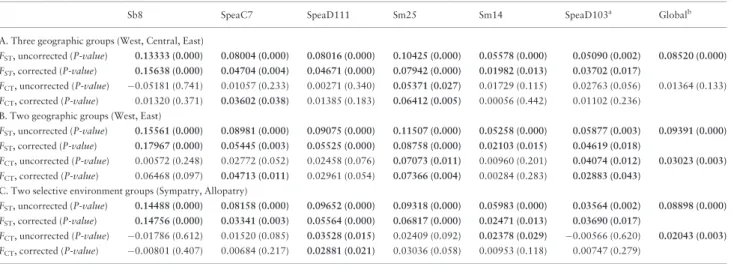
The optimal number of principal components to retain in our DAPC analyses varied among the population grouping schemes, with a minimum of seven principal components retained, and a maximum of 41 (for two and three geographic groups, respect-ively; Table 4). DAPC scatter plots indicated that the eastern populations were relatively distinct from the western and central
populations along the first discriminant function axis, while the western and central populations exhibited more subtle structure along the second discriminant function axis (Figure 2A). When grouping the populations into either two geographic or two select-ive environment groups, some separation was evident along the first discriminant function axis, but in both cases, substantial overlap remained (Figs. 2B and2C). Likewise, the proportion of overall correct assignment to original groups was higher for the three geographic groups than for the two geographic or two select-ive environment groups (Table 4). However, as expected, the rela-tive values of the proportion of overall correct assignment were dependent on the number of principal components retained in each DAPC (Table 4). To allow direct comparisons of correct as-signment proportions among the population grouping schemes, we calculated a mean proportion of overall correct assignment
based on assignments using the minimum and maximum optimal numbers of principal components (7 and 41 PCs, respectively;
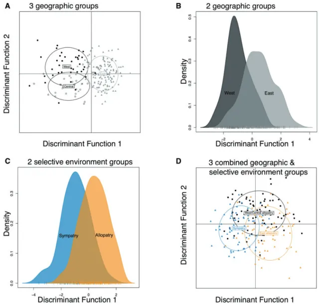
Table 4). This mean value was highest for the two geographic groups (Table 4). Breaking down the proportion of correct assign-ment by group when retaining the optimal number of principal components shows that the East geographic group is genetically distinct (Figure 3A and 3B) because of its accurate assignment. The proportion of correct reassignment to the West geographic group was higher when the Central population (HE) was not lumped in with the two populations farther west (SRV and EL;
Figure 3A and3B), suggesting that the HE population is slightly differentiated from EL and SRV. The higher proportion of correct reassignment for the Allopatry versus the Sympatry selective envir-onment groups (Figure 3C) is likely because the Allopatry group contains both West/Central and East populations, which are genet-ically distinct from each other (Figure 2A). The scatter plot for the combined geographic and selective environment grouping shows some separation between the Sympatry and Allopatry selective en-vironments along the first discriminant function axis (Figure 2D). This structure combined with the subtle separation between the West/Central allopatry populations and the remaining populations along the second discriminant function axis (Figure 2D) suggests that both geography and selective environment contribute to popu-lation differentiation.
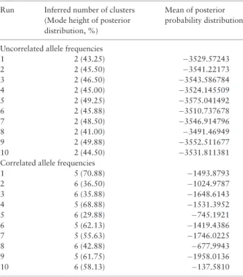
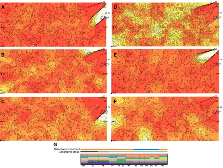
The two sets of 10 independent Geneland runs, using either the uncorrelated or the correlated allele frequency models, were consist-ent in the number of clusters inferred, with the uncorrelated allele frequency model inferring two clusters in all ten runs, and the corre-lated allele frequency model inferring either five or six clusters (Table 5). The consistency of inferred cluster number suggested that Geneland runs of at least 1,000,000 MCMC iterations were of ap-propriate length. In a single run of 2,000,000 MCMC iterations, the uncorrelated allele frequency model again inferred two genetic clus-ters (Figure 4). These clusters corresponded to the West and East population groups (Figs. 1and4). The correlated allele frequency model inferred the presence of six genetic clusters after a run of 2,000,000 MCMC iterations (Figure 5). However, the five clusters showed no clear correspondence to any geographic or selective en-vironment grouping (Figure 5).
Consistent with the DAPC results (Figure 2D), the two-factor AMOVA also indicated that both geographic grouping and selective environment explain the observed genetic variation (Table 6), but the higher partialR2value for geographic group suggested that this factor explains a greater proportion of the genetic variation than does selective environment. When the order of the factors is switched, both remain significant, and the partialR2remains higher for geographic group (data not shown). The overall MMRR model, however, was not significant (R2¼0.007, F¼0.179, P¼0.961),
suggesting that none of the three explanatory matrices—selective en-vironment contrast, Euclidean geographic distance, or environmen-tal cost distance—explained a significant amount of the variation in population pairwiseFSTat this scale. With the DAPC reassign-ment of YW population individuals to selective environreassign-ments, we found that 16 of 19 YW individuals were assigned to the allopatric selective environment (84.2%). This result was consistent with se-lective environment contributing to population structure at a more local scale.
Discussion
We evaluated the extent of population differentiation present at a re-gional scale among populations ofS. multiplicatathat are allopatric and sympatric with the congener,S. bombifrons. We then examined the relative contributions of divergent selective environments and geographic distance for explaining the observed population differentiation. To do this, we used multiple approaches to estimate population structure based on microsatellite genotypes from 13 populations, varying in selective environment and geographic loca-tion. Our hierarchical AMOVA (Table 3), DAPC (Table 4), two-fac-tor AMOVA (Table 6) and Geneland (Figure. 4) results indicate that geographic distance contributes more strongly to moderate popula-tion differentiapopula-tion across a regional scale. However, evidence from both the hierarchical (Table 3) and two-factor AMOVAs (Table 6), and the DAPC analyses (Figure 2D) also support a role for divergent selective environments, particularly at a more local scale.
Our estimates ofFSTindicate the presence of moderate popula-tion differentiapopula-tion, with estimates significantly higher than zero globally (FST0.09) and for each individual locus (Table 3). There was variation betweenFSTestimates that were and were not cor-rected for the presence of null alleles, as expected based on
simulation results (Chapuis and Estoup 2006) and our own previous work in this system (Rice and Pfennig 2010; Pfennig and Rice 2014). However, even after correcting for null alleles,FSTremained significantly greater than zero at every locus. Our finding of popula-tion differentiapopula-tion at this regional scale was consistent with our ex-pectations, based on S. multiplicata’s limited opportunities for dispersal and on previous research in this system at a smaller spatial scale (Rice and Pfennig 2008,2010;Rice et al. 2009,Pfennig and Rice 2014). However, the level of differentiation present among our populations was lower than expected for two reasons. First, a previ-ous study of local population structure among the EastS. multipli-catapopulations (Figure 1,Table 1) resulted inFSTvalues that were only slightly lower than estimates from this study (Pfennig and Rice 2014), even though the populations in this study span nearly six times the distance. Second, at similar or even smaller spatial scales, amphibian species often exhibit higher levels of population structure than what we found (Burns et al. 2004;Arens et al. 2006).
Several nonmutually exclusive factors can explain why the level of population differentiation inS. multiplicatawas lower than expected. First, the microsatellite markers we chose for this study were a subset of those used inPfennig and Rice (2014), which renders theFST esti-mates not directly comparable between the two studies. Additionally, the high variability of microsatellite markers can result in underesti-mates of population differentiation (Hedrick 1999). Second, it is pos-sible thatS. multiplicatahave a greater capacity for dispersal than many amphibian species. Although a moderate level of dispersal is likely among several of our East ponds because of the small distances separating them (<5 km), we think this is unlikely as a general ex-planation for our findings; this species lives in a desert environment, and spends much of the year hibernating in underground burrows (Bragg 1944, 1945). Finally, demographic factors, such as recent range expansions or large population sizes, can affect levels of popula-tion differentiation (Hewitt 2000; Johansson et al. 2006;
Wellenreuther et al. 2011). Genetic differentiation of the EastS. mul-tiplicatapopulations (Figure 1) based on mitochondrialcytochrome b sequences suggests that these populations have not undergone recent population growth or range expansion (Rice and Pfennig 2008). However, additional research is needed on the phylogeography and demography ofS. multiplicatapopulations across the species range to evaluate demographic history as an explanation for our findings.
Our results suggest that at a regional scale, geographic distance contributes more to the observed population differentiation inS. multiplicatathan does selective environment. The two geographic groups explained a greater proportion of the total variation in geno-type frequencies than did the three geographic or the two selective environment groups (Table 3). When the number of retained princi-pal components for DAPC was standardized across the three group-ing schemes, the two geographic groups had the highest mean proportion of overall correct assignment (Table 4). The higher par-tialR2value for geographic grouping in the two-factor AMOVA also suggest this factor explained more of the genetic variation (Table 6). Finally, the uncorrelated allele frequency model in Geneland inferred two genetic clusters (Figure 4A) with strong cor-respondence to the two geographic groups (Figure 4B). This result contrasts with contributions to population structure at a local scale;
Pfennig and Rice (2014)found that selective environment explained more of the population differentiation among the East populations (Figure 1) than did geography. Our finding that 84.2% of the indi-viduals from the YW population were assigned to the allopatric se-lective environment by a DAPC, even though located nearer to other sympatric populations, is consistent withPfennig and Rice (2014).
Table 5. Summary of independent Geneland runs under two mod-eling parameter sets
Run Inferred number of clusters (Mode height of posterior distribution, %)
Mean of posterior probability distribution
Uncorrelated allele frequencies
1 2 (43.25) 3529.57243
2 2 (45.50) 3541.22173
3 2 (46.50) 3543.586784
4 2 (45.00) 3524.145509
5 2 (49.25) 3575.041492
6 2 (45.88) 3510.737678
7 2 (48.50) 3546.914796
8 2 (41.00) 3491.46949
9 2 (49.88) 3552.511677
10 2 (44.50) 3531.811381
Correlated allele frequencies
1 5 (70.88) 1493.8793
2 6 (36.50) 1024.9787
3 6 (35.88) 1648.6143
4 5 (68.88) 1531.3952
5 6 (29.88) 745.1921
6 5 (62.13) 1419.4386
7 5 (55.63) 1746.0225
8 6 (42.88) 677.9943
9 5 (61.75) 1958.0136
Variation might often exist across a species’ range in the strength of particular evolutionary mechanisms, providing an explanation for why the key contributors to population differentiation have the potential to vary with spatial scale. For instance, populations of the European flounder at the edges of the species range exhibit genetic structuring and population sizes suggestive of founder events, while population structure in other parts of the range is more strongly associated with environmental or life history variation ( Hemmer-Hansen et al. 2007). As noted earlier, one possible explanation for the lower than expected population differentiation inS. multiplicata at this regional scale is that the populations from the geographic groups differ in their recent demographic histories. Demography is expected to affect the strength of both genetic drift and natural
selection is also present between the East allopatric and sympatric populations ofS. multiplicata. Ecological character displacement has occurred betweenS. multiplicataandS. bombifronsin tadpole morph production, resource use, and morphology (Pfennig and Murphy 2000;
Pfennig et al. 2007;Rice et al. 2009) in sympatric populations, but not in allopatric populations. This divergence in ecological selective pres-sures between sympatric and allopatric populations has led to extrinsic postzygotic reproductive isolation (Pfennig and Rice 2007). Hence, the balance between selection, genetic drift, and gene flow likely varies across different spatial scales inS. multiplicata, affecting patterns of population differentiation.
Although our results suggest that distance contributes more to population differentiation at a regional scale than does selective en-vironment, we found evidence that a portion of the population structure is associated with the divergent environments of allopatry and sympatry. The two selective environment groups exhibited a sig-nificant global weighted averageFCTvalue (Table 3). In addition, the DAPC illustrated some separation between allopatric and sym-patric population groups (Figs. 2C, 2D). When geographical group-ing and selective environment were considered simultaneously in the two-factor AMOVA, both were identified as significant contributors to genetic variation. Finally, individuals from the YW population were more frequently assigned to the correct selective environment group by DAPC than to the nearest geographic group. Using a dif-ferent analysis,Rice and Pfennig (2010)also found that YW was more genetically similar to other allopatric populations than to nearby sympatric populations.
That these presumably neutral microsatellite markers exhibit any structure associated with divergent selection is somewhat sur-prising. Although divergence due to selection can be detected with neutral markers (Rice and Pfennig 2010;Rosenblum and Harmon
Figure 5.Geneland results for the correlated allele frequency model. Run length was equal to 2,000,000 MCMC iterations, with six as the inferred number of clus-ters with the highest posterior probability. Heat maps illustrate the posterior probability of membership in A) cluster 1, B) cluster 2, C) cluster 3, D) cluster 4, E) cluster 5 and F) cluster 6. Lighter colors indicate higher posterior probability of membership in a given cluster. G) distruct plot visualizing the population assign-ment by Geneland, to each of the inferred clusters. Colors correspond to inferred clusters (orange, cluster 1; blue, cluster 2; yellow, cluster 3; pink, cluster 4; green, cluster 5; purple, cluster 6), with the height of each color indicating the probability of assignment to each inferred cluster. Individuals are grouped by sampling lo-cation (Table 1,Figure 1). Bars above the figure identify the selective environment group (allopatry, orange; sympatry, blue) and the geographic group (West, dark gray; Central, white; East, light gray) assignments for each population.
Table 6. Two-factor AMOVA testing the relative effects of geo-graphic group vs. selective environment on genetic distance
Factor df SS MS F PartialR2 P
Geographic group 1 11.6 11.6 13.1 0.06 <0.001 Selective environment 1 4.5 4.5 5.1 0.02 <0.001
Residuals 201 178.3 0.9 0.92
2011,Edelaar et al. 2012), theoretical and empirical results suggest that it often may not be (Crispo et al. 2006; Thibert-Plante and Hendry 2009,2010;Hoskin and Higgie 2010). Levels of genetic dif-ferentiation are expected to vary across the genome for populations that have adapted to divergent selective environments, with the highest levels of differentiation often present at and near loci involved in local adaptation and reproductive isolation (Nosil et al. 2009a;Cruickshank and Hahn 2014). Consistent with expectations of variable differentiation across the genome, only one to two of the six loci exhibited significantFCTs for sympatric versus allopatric population groups (Tables 3). Genome-wide studies will be neces-sary to evaluate the extent of genetic divergence between sympatric and allopatricS. multiplicatapopulations, and to identify specific loci associated with reproductive isolation and local adaptation.
In sum, our results indicate that at a regional scale, geographic distance contributes more to patterns of genetic differentiation amongS. multiplicatapopulations than does selective environment. This result contrasts with genetic structure in this species at a more local scale, which is associated with divergent selective environ-ments, and highlights the potential of reinforcement to initiate gen-etic differentiation. In general, variation across a species’ range in the balance of evolutionary forces at work can result in differences in the key contributors to genetic differentiation among locations and spatial scales.
Acknowledgments
The authors would like to thank R. Fuller for organizing and editing this spe-cial column on cascade reinforcement; E. Twomey and one anonymous re-viewer for helpful suggestions that greatly improved the article; D. and K. Pfennig for sharing tissue samples; and S. De La Serna Buzon for assistance with shipping the tissues. They are also very grateful to A. Chunco for sharing georeferenced occurrence locations ofS. multiplicatacompiled from museum records.
Funding
This research was funded by Lehigh University.
References
Adamack AT, Gruber B, 2014. PopGenReport: simplifying basic population genetic analyses in R.Methods Ecol Evol5:384–387.
Arens P, Bugter R, van’t Westende W, Zollinger R, Stronks J et al., 2006. Microsatellite variation and population structure of a recovering Tree frog
Hyla arboreaL.metapopulation.Conserv Genet7:825–835.
Arnegard ME, McGee MD, Matthews B, Marchinko KB, Conte GL et al., 2014. Genetics of ecological divergence during speciation.Nature511:307–311. Bewick ER, Dyer KA, 2014. Reinforcement shapes clines in female mate
dis-crimination inDrosophila subquinaria.Evolution68:3082–3094. Bradburd GS, Ralph PL, Coop GM, 2013. Disentangling the effects of
geo-graphic and ecological isolation on genetic differentiation. Evolution 67:3258–3273.
Bragg AN, 1944. The spadefoot toads in Oklahoma with a summary of our knowledge of the group.Am Nat78:517–533.
Bragg AN, 1945. The spadefoot toads in Oklahoma with a summary of our knowledge of the group. II.Am Nat79:52–72.
Brown JL, 2014. SDMtoolbox: a python-based GIS toolkit for landscape gene-tic, biogeographic and species distribution model analyses.Methods Ecol Evol5:694–700.
Burns EL, Eldridge MDB, Houlden BA, 2004. Microsatellite variation and population structure in a declining Australian HylidLitoria aurea.Mol Ecol 13:1745–1757.
Carlsson J, 2008. Effects of microsatellite null alleles on assignment testing.J Hered99:616–623.
Chapuis M-P, Estoup A, 2006. Microsatellite null alleles and estimation of population differentiation.Mol Biol Evol24:621–631.
Chunco AJ, Jobe T, Pfennig KS, 2012. Why do species co-occur? A test of al-ternative hypotheses describing abiotic differences in sympatry versus allop-atry using spadefoot toads.PLoS ONE7:e32748.
Coyne JA, Orr HA, 2004.Speciation. Sunderland, MA: Sinauer Associates. Crispo E, Bentzen P, Reznick DN, Kinnison MT, Hendry AP, 2006. The
rela-tive influence of natural selection and geography on gene flow in guppies.
Mol Ecol15:49–62.
Cruickshank TE, Hahn MW, 2014. Reanalysis suggests that genomic islands of speciation are due to reduced diversity, not reduced gene flow.Mol Ecol 23:3133–3157.
Edelaar P, Alonso D, Lagerveld S, Senar JC, Bjo¨rklund M, 2012. Population differentiation and restricted gene flow in Spanish crossbills: not isolation-by-distance but isolation-by-ecology.J Evol Biol25:417–430.
Etherington TR, 2011. Python based GIS tools for landscape genetics: visualiz-ing genetic relatedness and measurvisualiz-ing landscape connectivity.Methods Ecol Evol2:52–55.
Excoffier L, Lischer HEL, 2010. Arlequin suite ver 3.5: a new series of pro-grams to perform population genetics analyses under Linux and Windows.
Mol Ecol Resource10:564–567.
Fitzpatrick BM, 2009. Power and sample size for nested analysis of molecular variance.Mol Ecol18:3961–3966.
Fuller RC, 2008. Genetic incompatibilities in killifish and the role of environ-ment.Evolution62:3056–3068.
Gaggiotti OE, Lange O, Rassmann K, Gliddon C, 1999. A comparison of two indirect methods for estimating average levels of gene flow using microsatel-lite data.Mol Ecol8:1513–1520.
Guillot G, 2008. Inference of structure in subdivided populations at low levels of genetic differentiation: the correlated allele frequencies model revisited.
Bioinformatics24:2222–2228.
Guillot G, Estoup A, Mortier F, Cosson JF, 2005. A spatial statistical model for landscape genetics.Genetics170:1261–1280.
Guillot G, Santos F, Estoup A, 2008. Analysing georeferenced population genetics data with Geneland: a new algorithm to deal with null alleles and a friendly graphical user interface.Bioinformatics24:1406–1407.
Hatfield T, Schluter D, 1999. Ecological speciation in sticklebacks: environ-ment-dependent hybrid fitness.Evolution53:866–873.
Hedrick PW, 1999. Highly variable loci and their interpretation in evolution and conservation.Evolution53:313–318.
Hemmer-Hansen J, Nielsen EE, Grønkjaer P, Loeschcke V, 2007. Evolutionary mechanisms shaping the genetic population structure of mar-ine fishes; lessons from the European flounder (Platichthys flesusL.).Mol Ecol16:3104–3118.
Hewitt G, 2000. The genetic legacy of the Quaternary ice ages. Nature 405:907–913.
Hijmans RJ, Cameron SE, Parra JL, Jones PG, Jarvis A, 2005. Very high reso-lution interpolated climate surfaces for global land areas.Int J Climatol 25:1965–1978.
Hoskin CJ, Higgie M, 2010. Speciation via species interactions: the divergence of mating traits within species.Ecol Lett13:409–20.
Hoskin CJ, Higgie M, McDonald KR, Moritz C, 2005. Reinforcement drives rapid allopatric speciation.Nature437:1353–1356.
Jaenike J, Dyer KA, Cornish C, Minhas MS, 2006. Asymmetrical reinforce-ment and Wolbachia infection inDrosophila.PLoS Biol4:e325.
Jiggins CD, Estrada C, Rodrigues A, 2004. Mimicry and the evolution of pre-mating isolation inHeliconius melpomeneLinnaeus.J Evol Biol17: 680– 691.
Johansson M, Primmer CR, Merila¨ J, 2006. History vs. current demography: explaining the genetic population structure of the common frogRana tem-poraria.Mol Ecol15:975–983.
Jombart T, 2008. adegenet: a R package for the multivariate analysis of genetic markers.Bioinformatics24:1403–1405.
Jombart T, Devillard S, Balloux F, 2010. Discriminant analysis of principal components: a new method for the analysis of genetically structured popula-tions.BMC Genet11:94.
Kalinowski ST, 2005. Do polymorphic loci require large sample sizes to esti-mate genetic distances?Heredity94:33–36.
Kosman E, Leonard KJ, 2005. Similarity coefficients for molecular markers in studies of genetic relationships between individuals for haploid, diploid, and polyploidy species.Mol Ecol14:415–424.
Lemmon EM, 2009. Diversification of conspecific signals in sympatry: geo-graphic overlap drives multidimensional reproductive character displace-ment in frogs.Evolution63:1155–1170.
McPeek MA, Gavrilets S, 2006. The evolution of female mating preferences: differentiation from species with promiscuous males can promote speci-ation.Evolution60:1967–1980.
Nanninga GB, Saenz-Agudelo P, Manica A, Berumen ML, 2014. Environmental gradients predict the genetic population structure of a coral reef fish in the Red Sea.Mol Ecol23:591–602.
Nosil P, Egan SP, Funk DJ, 2008. Heterogeneous genomic differentiation be-tween walking-stick ecotypes: “isolation by adaptation” and multiple roles for divergent selection.Evolution62:316–336.
Nosil P, Funk DJ, Ortiz-Barrientos D, 2009a. Divergent selection and hetero-geneous genomic divergence.Mol Ecol18:375–402.
Nosil P, Harmon LJ, Seehausen O, 2009b. Ecological explanations for (incom-plete) speciation.Trends Ecol Evol24:145–156.
Nosil P, Vines TH, Funk DJ, 2005. Perspective: reproductive isolation caused by natural selection against immigrants from divergent habitats.Evolution 59:705–719.
Oksanen J, Blanchet FG, Kindt R, Legendre P, Minchin PR et al., 2015. vegan: Community Ecology Package. R package version 2.3-2 [cited 2016 January 10]. Available from: http://CRAN.R–project.org/package¼vegan. Ortiz-Barrientos D, Grealy A, Nosil P, 2009. The genetics and ecology of
re-inforcement: implications for the evolution of prezygotic isolation in sym-patry and beyond.Ann NY Acad Sci1168:156–182.
Pfennig DW, Murphy PJ, 2000. Character displacement in polyphenic tad-poles.Evolution54:1738–1749.
Pfennig DW, Murphy PJ, 2002. How fluctuating competition and phenotypic plasticity mediate species divergence.Evolution56:1217–1228.
Pfennig DW, Pfennig KS, 2012. Evolution’s wedge: competition and the ori-gins of diversity. Berkeley: University of California Press.
Pfennig DW, Rice AM, 2007. An experimental test of character displace-ment’s role in promoting postmating isolation between conspecific popu-lations in contrasting competitive environments. Evolution61:2433– 2443.
Pfennig DW, Rice AM, Martin RA, 2007. Field and experimental evidence for competition’s role in phenotypic divergence.Evolution61:257–271. Pfennig KS, 2000. Female spadefoot toads compromise on mate quality to
en-sure conspecific matings.Behav Ecol11:220–227.
Pfennig KS, 2003. A test of alternative hypotheses for the evolution of repro-ductive isolation between spadefoot toads: support for the reinforcement hypothesis.Evolution57:2842–2851.
Pfennig KS, Allenby A, Martin RA, Monroy A, Jones CD, 2012. A suite of mo-lecular markers for identifying species, detecting introgression and describ-ing population structure in spadefoot toads (Speaspp.).Mol Ecol Resource 12:909–917.
Pfennig KS, Rice AM, 2014. Reinforcement generates reproductive isolation between neighbouring conspecific populations of spadefoot toads.Proc R Soc B281:20140949.
Pfennig KS, Ryan MJ, 2006. Reproductive character displacement generates reproductive isolation among conspecific populations: an artificial neural network study.Proc R Soc B273:1361–1368.
Pfennig KS, Simovich MA, 2002. Differential selection to avoid hybridization in two toad species.Evolution56:1840–1848.
Phillips S, Anderson R, Schapire R, 2006. Maximum entropy modeling of spe-cies geographic distributions.Ecol Model190:231–259.
Porretta D, Urbanelli S, 2012. Evolution of premating reproductive isolation among conspecific populations of the sea rock-pool beetle Ochthebius
urbanelliae driven by reinforcing natural selection.Evolution 66:1284– 1295.
Pruett CL, Winker K, 2008. The effects of sample size on population genetic diversity estimates in song sparrows Melospiza melodia. J Avian Biol 39:252–256.
R Core Team, 2015. R: A Language and Environment for Statistical Computing. Vienna: R Foundation for Statistical Computing.
Raymond M, Rousset F, 1995. GENEPOP (version 1.2): population genetics software for exact tests and ecumenicism.J Hered86:248–249.
Rice AM, Leichty AR, Pfennig DW, 2009. Parallel evolution and ecological selection: replicated character displacement in spadefoot toads.Proc R Soc B276:4189–4196.
Rice AM, Pearse DE, Becker T, Newman RA, Lebonville C et al., 2008. Development and characterization of nine polymorphic microsatellite markers for Mexican spadefoot toadsSpea multiplicatawith cross-amplifica-tion in Plains spadefoot toadsS. bombifrons.Mol Ecol Resource8:1386– 1389.
Rice AM, Pfennig DW, 2008. Analysis of range expansion in two species undergoing character displacement: why might invaders generally “win” during character displacement?J Evol Biol21:696–704.
Rice AM, Pfennig DW, 2010. Does character displacement initiate speciation? Evidence of reduced gene flow between populations experiencing divergent selection.J Evol Biol23:854–865.
Rosenberg NA, 2004. DISTRUCT: a program for the graphical display of population structure.Mol Ecol Notes4:137–138.
Rosenblum EB, Harmon LJ, 2011. “Same same but different”: replicated eco-logical speciation at White Sands.Evolution65:946–960.
Rousset F, 2008. Genepop ’007: a complete reimplementation of the Genepop software for Windows and Linux.Mol Ecol Resource8:103– 106.
Rundle HD, Nosil P, 2005. Ecological speciation. Ecol Lett 8:336– 352.
Schluter D, 2001. Ecology and the origin of species.Trends Ecol Evol16:372– 380.
Sexton JP, Hangartner SB, Hoffmann AA, 2014. Genetic isolation by environ-ment or distance: which pattern of gene flow is most common?Evolution 68:1–15.
Shafer ABA, Wolf JBW, 2013. Widespread evidence for incipient ecological speciation: a meta-analysis of isolation-by-ecology.Ecol Lett16:940– 950.
Simovich MA, Sassaman CA, 1986. Four independent electrophoretic markers in spadefoot toads.J Hered77:410–414.
Snowberg LK, Benkman CW, 2007. The role of marker traits in the assortative mating within red crossbills Loxia curvirostra complex. J Evol Biol 20:1924–1932.
Stebbins RC, 2003.A Field Guide to Western Reptiles and Amphibians. New York: Houghton Mifflin Company.
Svensson EI, Eroukhmanoff F, Friberg M, 2006. Effects of natural and sexual selection on adaptive population divergence and premating isolation in a damselfly.Evolution60:1242–1253.
Thibert-Plante X, Hendry AP, 2009. Five questions on ecological speci-ation addressed with individual-based simulspeci-ations.J Evol Biol22:109– 123.
Thibert-Plante X, Hendry AP, 2010. When can ecological speciation be de-tected with neutral loci?Mol Ecol19:2301–2314.
Van Den Bussche RA, Lack JB, Stanley CE, Wilkinson JE, Truman PS et al., 2009. Development and characterization of 10 polymorphic tetranucleotide microsatellite markers for New Mexico spadefoot toadsSpea multiplicata.
Conserv Genet Resour1:71–73.
Van Oosterhout C, Hutchinson WF, Wills DPM, Shipley P, 2004. Micro-Checker: software for identifying and correcting genotyping errors in micro-satellite data.Mol Ecol Notes4:535–538.
Via S, 2009. Natural selection in action during speciation. PNAS 106(Suppl):9939–9946.
quantifying geographic and ecological isolation.Dryad Digital Repository. http://dx.doi.org/10.5061/dryad.kt71r.
Wang IJ, 2013b. Examining the full effects of landscape heterogeneity on spatial genetic variation: a multiple matrix regression approach for quantifying geo-graphic and ecological isolation.Evolution67:3403–3411.
Wang IJ, Summers K, 2010. Genetic structure is correlated with phenotypic di-vergence rather than geographic isolation in the highly polymorphic straw-berry poison-dart frog.Mol Ecol19:447–458.
Wellenreuther M, Sanchez-Guille´n RA, Cordero-Rivera A, Svensson EI, Hansson B, 2011. Environmental and climatic determinants of molecular di-versity and genetic population structure in a coenagrionid damselfly.PLoS ONE6:e20440.