Atlas diffeomorphisms via object models

(1)

Atlas Diffeomorphisms via Object Models

Rohit R. Saboo

A dissertation submitted to the faculty of the University of North Carolina at Chapel Hill in partial fulfillment of the requirements for the degree of Doctor of Philosophy in the Depart-ment of Computer Science.

Chapel Hill 2012

Approved by:

Stephen M. Pizer, Advisor

Julian G. Rosenman, Reader

Jack Snoeyink, Reader

Ron Alterovitz, Reader

(2)

(3)

Abstract

ROHIT R. SABOO: Atlas Diffeomorphisms via Object Models. (Under the direction of Stephen M. Pizer.)

To tackle the problem of segmenting several closely-spaced objects from 3D medical im-ages, I propose a hybrid of two segmentation approaches: one image-based and one model-based. A major contribution takes the image-based approach by diffeomorphically mapping a fully segmented atlas image to a partially segmented target patient image preserving any ‘correspondence’ inferred from the partial segmentation of the target. The mapping is pro-duced by solving the steady-state heat flow equation where the temperature is a coordinate vector and corresponding points have the same temperature. Objects carried over from the atlas into the target serve as reasonable initial segmentations and can be further refined by a model-based segmentation method. Good quality segmentations are added to the list of the initial partial segmentations, and the process is repeated.

Another contribution takes the model-based approach in developing shape models of quasi-tubular objects and statistics on those models. Whereas medial models were previously only developed for slab-shaped objects, this contribution provides an approximately medial method to stably represent nearly tubular objects.

(4)

List of Tables

5.1 Average initial, final, and decrease in the median of the surface dis-tances for several organs by enhancing the m-rep fit using a heat flow

based method. . . 65

5.2 Average ensemble entropy and movement for the points. The length

of a side of a voxel is approximately0.4mm. . . 69 7.1 Match measures between atlas reference objects and warped

refer-ence objects from the patient image. . . 99

7.2 Match measures between atlas target objects and warped target

ob-jects from the patient image. . . 99

7.3 Match measures between atlas target objects and warped target ob-jects from the patient image after the sternocleidomastoid muscle was

added to the list of reference objects. . . 99

8.1 Mean and standard deviation over the11random pairs of patients, of the volume overlaps of each of the different objects used to determine

the warp by the method in section 8.1. . . 108

8.2 Mean and standard deviation of volume overlaps of each of the differ-ent objects on which the warp introduced in section 8.1 was applied. For structures for which I had only one sample, only the mean is listed

(9)

List of Figures

1.1 An overview of the hierarchical warp method: The labeled mesh gen-erator and the surface correspondence method are shown in fig. 1.2 and 1.3 respectively. The rounded rectangles represent processes, or-dinary rectangles are inputs and outputs, and rectangles with a double

left edge are precomputed inputs. . . 5

1.2 An overview of the method that generates labeled meshes from binary

images. . . 7

1.3 An overview of the entropy-based correspondence system that takes in labeled meshes from the atlas and the patient and returns meshes

in correspondence. . . 8

2.1 Lymphatics of the head and neck (obtained from Gray’s anatomy 1918) . 14

2.2 Three different nodal levels on an axial slice from a head and neck CT scan 15

2.3 Metal streak artifacts in a head and neck CT image . . . 15

2.4 Some of the segmented head and neck organs with the Level-III nodal region 16

3.1 A medial atom. . . 19

3.2 An m-rep model of the medial scalene muscle showing the grid of medial atoms. The atoms at the edges of the grid are special – they are coalesced from an ordinary atom and one that is on the edge of

the continuous medial sheet. . . 19

3.3 Correspondence between points on the surface of two different thyroids. . 23

3.4 A 2D slice from a 3D CT scan in the application of thin plate spline registration between two different patients: The level III lymph levels carried over in the registration are drawn in green. Notice that they

are folded. . . 26

3.5 Solution of Laplace’s equation: The top and bottom curves are fixed value boundary surfaces. Solid lines indicate equi-potential lines, and

(10)

4.1 A cross-section through a nearly tubular object. As the cross-section marginally changes, the orientation of the medial surface changes by

90◦ depicting the instability in representing a nearly tubular object

with a slab-shaped m-rep. . . 34

4.2 Renderings of quasi-tube models fitted to different objects. From the left to right the objects are sections of the head and neck’s skin surface extracted from a 3D CT scan, the carotid artery, the internal jugular vein, and a section of the upper airway. . . 34

4.3 Representation of a tube atom . . . 42

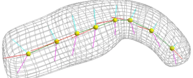
4.4 A mean model of a rectum from one of our studies showing the me-dially implied surface as a wireframe. . . 42

4.5 Surface of a twisted bowling pin . . . 45

4.6 Surface of the same bowling pin, now untwisted . . . 45

4.7 The structure of a medial atom. . . 46

4.8 Mean model of a rectum (center) deformed by±1.5standard devia-tions along the first mode of variation (left and right), which resem-bles the anatomical shape change due to bloating by gas. . . 48

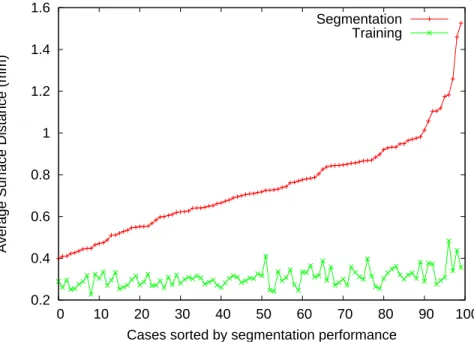
4.9 Set of segmentation results in decreasing order of performance on synthetic rectum images: The segmented rectum is shown in a gray color, and the ground truth is shown by a transluscent blue color. The average distances between the two from left to right in units of mm are: 0.9, 1.2, 1.4, and 4.0. . . 50

4.10 The red line shows the average distance our segmentation results were from the ground truth on synthetic rectum data. The green line shows the same for the trained models. The length of a side of a voxel is2mm. . 50

4.11 A quasi-tube atom with spokes of varying length and a cut-away sec-tion of the medially implied surface shown in two different orientasec-tions. . 51

4.12 Average surface distance between the training models and the expert segmentation for the several cases (sorted by increasing performance of the coarse tube model) at different stages of fitting – coarse tube fitting, coarse quasi-tube fitting, and finer scale quasi-tube fitting. . . 54

(11)

4.14 Boxplot of distribution of segmentation results versus training results. The box goes from25% to75% quartile with a line for the median. The two lines at the end go1.5times the intra-quartile range (except

when there is no more data). The red dots are outliers. . . 55

4.15 Each row shows the outline (white or black) of our segmentation on two different axial slices of the same image. Note the poor contrast in the slices in the right column. The slices on the right are inferior with respect to those on the left. The first three rows are typical results,

and the last row is one of the better segmentations. . . 56

4.16 Quasi-tubular medial models (in white) fit to sections of the head and neck skin surface (left), common carotid arteries (top right), and upper airway sections (bottom right) vs. the manually segmented

ob-jects (in translucent blue) . . . 57

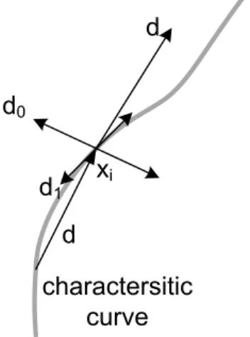
5.1 Three of the four differencing directions at pointxi: d0 andd1 are

orthogonal todalong which∇T|xi is computed. . . 63

5.2 A lateral view of a mandible with the condyles enclosed in a box (left), zoomed in versions of the condyles – lateral view (center) and anterior view (right). The condyles are typically a voxel thick and

pose numerical issues for the heat flow method. . . 64

5.3 A manually segmented mandible. Note the severe aliasing. . . 67

5.4 An anti-aliased version of the mandible shown on the left. . . 67

5.5 Corresponding points after entropy-based correspondence between

tracheas of six different patients. . . 69

left clavicle bones of six different patients. . . 70

right clavicle bones of six different patients. . . 71

mandibles of six different patients. . . 72

6.1 A pointpis shown with its neighboring pointsn0. . .n4 in the space of the target image. The colors range from black for a low tempera-ture to red for a high temperatempera-ture. The gray arrow shows the direction

(12)

6.2 Subdivision of a cube into five tetrahedra: abed, hedg, befg, bcgd, and gbde. a,b,c,d,e,f,g, and h are points on the grid where the warp is

computed. . . 79

6.3 A cross-section of a warp field through successive iterations begin-ning with the top-left progressing to the bottom right. Folds surround-ing the central region, seen by tangencies of the almost horizontal and almost vertical grid lines) go away with progressing iterations. The

warp field on the bottom left has no folded volume. . . 82

6.4 The standard deviation and the maximum deviation of the concentric spheres from a spherical shape in a warp field between two spheres as the outer sphere was scaled by a factorα. The data is presented in

units of image voxels. . . 83

6.5 The mean and the standard deviation of the distance moved by points along the surface of concentric spheres from their true position in a warp field between two spheres as the outer sphere was scaled by a

factorα. The data is presented in units of image voxels. . . 84 6.6 The radii of the warped concentric spheres as a function (solid line)

of their original radii in a warp field between two spheres as the outer sphere was scaled by a factorα = 2.0. The data is presented in units of image voxels. The ideal relationship is shown by the dotted line.

The relationship is almost linear and close to the ideal relationship. . . 85

7.1 Reference objects. In the case of the skin, only the section below the

bridge of the nose and above the top of the neck is used. . . 91

7.2 Landmarks on the skin surface shown on a sagittal slice of a CT image

of a patient. . . 92

7.3 Target objects . . . 93

7.4 Atlas’ skin surface in blue with the warped patient’s skin surface over-laid in red. Most of the two surfaces match well. However, the nose of the atlas patient has been arbitrarily cut off, and the match near the nose is poor. Also, the ears are very thin and variable across patients,

and the match near the ears is also poor. . . 94

7.5 Atlas’ mandible in blue with the warped patient’s mandible overlaid in red. Most of the warped mandible matches with the atlas mandible. However, the condyles that do not match well because of the difficulty

(13)

7.6 Atlas’ trachea in blue with the warped patient’s trachea overlaid in

red. The two surfaces match well almost everywhere. . . 96

7.7 Atlas’ left clavicle in blue with the warped patient’s left clavicle

over-laid in red. The two surfaces match well almost everywhere. . . 97

7.8 Atlas’ right clavicle in blue with the warped patient’s right clavicle

overlaid in red. The two surfaces match well almost everywhere. . . 98

7.9 Internal jugular veins in the atlas (blue), warped from patient image (red), and warped from patient image after using the sternocleidomas-toid muscle as a reference object (cyan). The image on the left shows the results on different axial slices. The images on the right show the same in 3D. There is a noticeable improvement in the match between the warped internal jugular vein and the atlas from when the stern-ocleidomastoid muscle was not used as an additional reference object

(top right) to when it was (bottom right). . . 100

7.10 Masseter muscle in the atlas (blue), warped from patient image (red), and warped from patient image after using the sternocleidomastoid muscle as a reference object (cyan). The image on the left shows the results on different axial slices. The images on the right show the same in 3D. The masseter muscle is adjacent to the mandible, which is a reference object. The warped masseter appears to match reason-ably well with the atlas masseter. Further, there is not much improve-ment from when the sternocleidomastoid muscle was not used as an

additional reference object (top right) to when it was (bottom right). . . . 101

7.11 Thyroid in the atlas (blue), warped from patient image (red), and warped from patient image after using the sternocleidomastoid mus-cle as a reference object (cyan). The image on the left shows the results on different axial slices. The images on the right show the same in 3D. The thyroid lies next to the trachea. The warped thyroid appears to match reasonably well with the atlas thyroid. There is not much improvement from when the sternocleidomastoid muscle was not used as an additional reference object (top right) to when it was

(bottom right). . . 102

7.12 Right sternocleidomastoid muscle in the atlas (blue) and warped from patient image (red). The image on the left shows the results on dif-ferent axial slices. The image on the right shows the same in 3D. The

(14)

8.1 Initial temperature distribution for the two temperature components on a spherical surface. All points on a latitude are assigned the same temperature value. The poles are separated as far apart as possible for

(15)

Chapter 1 Introduction

1.1 The Segmentation Challenge

Several real world applications, such as surgical planning and radiotherapy treatment plan-ning, require segmentation, or the outlining of objects in three-dimensional (3D) medical images. Automatic segmentation is a challenging, well-studied problem for which several solutions have been proposed. Most solutions are designed with specific applications in mind and are difficult to generalize.

(16)

• Image-based approaches:

These methods start from an image of an “average”1 _{patient, referred to as the} _atlas image. This image is carefully segmented by experts. When a new patient’s image2 _is ready for segmentation, the atlas image is warped into the new image using information such as geometric and intensity features. This warp is used to map the segmentations in the atlas image into the new image. Most existing work optimizes the warp by matching intensity features.

The main problem that these methods suffer from is that this optimization happens in a very high-dimensional space. Thus, almost always, one has to use local, greedy methods to do the optimization so that it finishes in a timely manner. This makes the methods susceptible to image artifacts.

• Model-based approaches:

These methods use a combination of a geometric model and image intensity features to model a shape and then segment the object from the image.

Such methods suffer from two problems: First, segmenting one organ at a time does not respect interdependencies between neighboring objects. This can lead to undesirable overlap in segmentation results.

Second,allmodel-based methods optimize an objective function that is typically com-posed of some geometric and image features. These objective functions are normally not convex, and the number of parameters involved is quite high. As a result, begin-ning from an initial estimate, they can get stuck in local minima. The better the initial estimate, the better are the chances of getting an accurate segmentation. These initial-izations typically involve some manual labor and can be very tedious for a complex of about40objects.

1_{The word average is used in a loose sense and could simply be the most typical patient or even a choice from}

among typical patients from various classes.

(17)

Both classes of methods can lead to poor correspondences between matching points on the atlas and the target that can in turn lead to poor segmentations. In the next section, I give an overview of my method, which borrows from both of these classes and can deliver segmentations of a complex of objects. It employs correspondence-preserving warps from partially segmented atlases, which is a geometry-based warping method that does not use image intensities and is therefore not afflicted by some of the problems faced by a warping-based method. It then segments the organs using a model-warping-based method, where most of the work is done by the previous step, thereby reducing the chances of getting stuck in a local minimum or neighboring objects overlapping each other after segmentation. This combination of the two brings out the best of both approaches.

1.2 Overview

(18)

warping method.

In the next few paragraphs, I give a brief overview of all the requirements of the warp-ing method and how each of them is met. In section 1.5 and fig. 1.1, I describe how this correspondence-preserving warping method is embedded in a larger framework to segment a complex of objects. The method is also presented in the form of an algorithm (1).

Algorithm 1Hierarchical segmentation algorithm Require: patient image

Require: shape models

Require: segmented atlas image with labeled surface meshes return segmented patient image (for organs with shape models) Reference objects list←{easily segmentable objects}

Target objects list←{objects to be segmented} repeat

for allobject∈Reference objects listdo

Generate labeled mesh of object in patient image.

Compute correspondence between object mesh in patient image and atlas image. end for

Produce a correspondence-preserving warphbetween patient image and atlas image. for allobject∈Target objects listdo

warped object←apply warphto object.

Segment object by initializing segmentation method with warped object. ifobject is segmented wellthen

Reference objects list←Reference objects list∪{object} Target objects list←Target objects list−{object}

end if end for

untilSegmentations are satisfactory or no improvement is seen.

The larger framework, which segments a complex of objects, starts with a fully segmented atlas. The atlas is augmented with the shape models of all the objects that we wish to segment. The labeled mesh generator, discussed in section 1.3, partially segments the target to produce surface meshes with labeled vertices. These objects, which are also easily segmented in the target because of high contrast, are calledreference objects, and the remaining not so easily-segmented objects are calledtarget objects.

(19)

Patient Image

Labeled Mesh Generator

Apply Warp

Segmented Atlas Image With

Labeled Surface Meshes

Shape Models

Target Objects List

Reference Objects List

Surface Correspondence Patient Reference

Surface Meshes With Labeled Vertices

Correspondence-preserving Warp Atlas and Patient Reference Meshes in Correspondence

Warp

Initialized Shape Models

Segment

Segmentation Results Select good

results

-+

(20)

repositioned vertices on the reference objects in the atlas and the target. Next, I use these correspondences to drive a warp from the atlas to the target image in my correspondence-preserving warping method; the warp from the correspondence-correspondence-preserving warping method is based purely on geometric information learned from meshes of the reference objects. These steps are discussed in sections 1.3 and 1.4 respectively.

The resulting warp gives us an initial guess for the segmentation of the target objects. The objects are segmented, and good results are selected. This thesis does not discuss the method of model-based segmentation; Broadhurst [4] and Stough [33] provide details on a particularly efficacious appearance model. The good results, segmentations that appear to match well with the image, are added to the list of the reference objects and removed from the list of the target objects. This loop is called the hierarchical warp method.

1.3 Overview of the Correspondence Method

The inputs and outputs for the correspondence method are as follows:

• Inputs – smooth segmentations of the reference objects in both atlas and target patient images;

• Outputs – correspondence labels on surface points on the same segmentations in both the atlas and the target patient images.

(21)

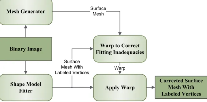
Binary Image Mesh Generator

Shape Model Fitter

Warp to Correct Fitting Inadequacies

Surface Mesh With Labeled Vertices

Apply Warp

Warp Surface

Mesh

Corrected Surface Mesh With Labeled Vertices

Figure 1.2: An overview of the method that generates labeled meshes from binary images.

not accurate enough for the correspondence-preserving warping method and is improved by an entropy-based correspondence method, shown in fig. 1.3, that moves the individual points on the surface. The entropy-based correspondence method can sometimes get stuck in local minima and initializing it in this manner can yield improved results.

The entropy-based correspondence method requires the computation of curvatures on the surface of objects. To robustly compute surface curvatures, any aliasing artifacts present in the mesh should be removed. A mesh extracted from a binary image is always aliased and needs to be anti-aliased. This necessitates the use of an anti-aliasing procedure on the mesh. I have developed a method that anti-aliases such meshes by a a fourth-order Laplacian of curvature flow.

(22)

Patient Surface Mesh With Labeled Vertices

Entropy-based

Correspondence Warp Apply Warp

Atlas and Patient Surface Meshes in

Correspondence Atlas Surface

Mesh With Labeled Vertices

Figure 1.3: An overview of the entropy-based correspondence system that takes in labeled meshes from the atlas and the patient and returns meshes in correspondence.

by the use of an entropy-based correspondence algorithm developed by Oguz et al. [28]. Some objects in the body are tube-like and others are slab-like. Existing work on m-reps can only represent slab-like objects. We need similar abilities of modeling and computing correspondence between tube-like objects that we have for slab-like objects. A method that can model tube-like objects that is consistent with the manner in which slab-like objects can be modeled has been developed, as described in chapter 4.

1.4 Correspondence-preserving Warping Method Overview

The inputs and outputs for the correspondence-preserving warping method are as follows:

• Inputs – segmentations (in the form of boundary meshes) of the reference objects in both the atlas and the target patient’s images with correspondence labels;

• Output – a mapping between the atlas and the target patient’s image.

(23)

for each dimension, and they are all independent of one another. This is imposed as a bound-ary condition in the target image; in addition, another set of boundbound-ary conditions is imposed at the actual boundaries of the target image. With these boundary conditions, we solve the steady-state heat equation. As a result of solving this equation, a point in the atlas will have a corresponding point in the target image with the same set of temperatures. This correspon-dence is used to map points between the atlas and the target images.

We also let the heat conduction coefficient vary across the image while solving the heat equation. The precise way in which this is done will be detailed later. Doing so ensures that the mapping between the two images is smooth and is devoid of folds. I will refer to such a mapping asalmost diffeomorphic.

In the next section, I show how this method is embedded in a larger framework that can segment objects.

1.5 Hierarchical Warp

The inputs and outputs for the hierarchical warping method are as follows:

• Inputs – the target patient’s image and a fully segmented atlas image augmented with shape models of the objects;

• Output – a fully segmented target image.

We first identify high-contrast objects that can be easily segmented, such as air cavities and bones. In the image from the target patient, we first segment these easily identifiable objects. These objects form the initial set of the reference objects.

The method described above is then used to infer a warp between the atlas and the target patient. At a result of its application, we have accurate initial guesses for the location of each of the objects.

(24)

The segmentations results are automatically evaluated and some of them are now chosen as new reference objects and the whole process is repeated again.

In fig. 1.1, I have presented a graphical overview of this hierarchical segmentation ap-proach.

1.6 Thesis and Claims

Thesis: Atlas-based segmentation methods that use correspondence produce superior results on a complex of interrelated objects than those that do not. Methods that establish good

correspondence, when combined with methods that produce a warp using the steady-state

heat equation, efficaciously provide the required correspondence-based warps leading to good

segmentations.

The contributions of this dissertation are the following:

1. The dissertation develops a method, based on heat flow in 4D space, to interpolate between the boundaries of pairs of objects while respecting correspondence. (This is different from the method sketched in section 1.4 and claim2below.)

2. Interpolation of objects while warping is not always required; most of the time, we only care about the end result of the warp. My warp method, based on heat flow in 3D space, is guaranteed to produce a smooth, non-folded warp between the two images while respecting positional correspondences on object surfaces; it has been developed out of a desire to provide better guarantees and efficiency than the method described under claim1.

3. Modeling nearly tubular objects by conventional medial models is not stable. My quasi-tubular models represent objects that are nearly quasi-tubular in shape, giving reasonable cor-respondence and stable probability distributions on their shape spaces.

(25)

try to model the object at a large scale. This can be a problem when they are used as the basis of a warping mechanism. My method based on heat flows improves the correspondence by moving the points to the actual surface when using shape models, specifically m-reps.

5. The correspondence implied by m-reps may not be good enough for correspondence-based warping methods. Even after the points have been moved to the correct surface, they may still need to slide along the surface. My method based on Oguz et al. [28] improves this correspondence.

6. The head and neck area is a challenge for 3D image segmentation. My framework, using the methods developed, can deliver reasonable initializations for segmentation of certain objects (masseter muscle, sternocleidomastoid muscle, and thyroid) in 3D head and neck CT images.

7. Binary images can be efficaciously anti-aliased by a fourth-order Laplacian of curvature flow.

1.7 Overview of Chapters

This chapter provided a brief overview of correspondence-preserving warping methods, their prerequisites, and the manner in which they can be embedded in a larger framework to produce quality segmentations.

In chapter 2, I present the medical problem, head and neck segmentation, that drove the development of this method. I also discuss how existing methods may not live up to challenges presented to us.

Chapter 3 gets the reader up to speed on concepts that include m-reps, thin plate splines, and existing work on registration using partial differentiation equations.

(26)

nearly tubular-shaped cannot be modeled effectively by the same methods. In chapter 4, I discuss how to model nearly tubular objects and represent populations of them, and in doing so realize claim3. These medial models provide an initial approximate correspondence between objects in the atlas image and the patient image.

Chapter 5 discusses the two types of correspondence-enhancing methods: moving points from the m-rep-implied surface to the correct surface, and moving points along the surface. This chapter establishes claims4and5.

In chapter 6 I develop two methods to warp a volume into another volume by respecting correspondence between matching surfaces: The first one solves a heat equation in4 dimen-sions; it warps and produces interpolations between the two volumes. This establishes claim1. The second method solves a heat equation in 3dimensions; it produces a warp between the two volumes. In doing so, claim2is established.

(27)

Chapter 2 Application

In section 2.1, I present the medical problem of head and neck cancer. which provides the main driving problem for this dissertation. Section 2.2 follows with a discussion of why segmentation for treatment planning in head and neck cancer is challenging.

2.1 Treatment of Head and Neck Cancer

There are approximately 40,000 cases of cancers of the head and neck diagnosed each year in the United States. These tumors are usually sensitive to radiation and chemotherapy, and are often treated with both modalities. Several objects in the head and neck are at risk from receiving too much radiation; the parotid (salivary) glands are particularly sensitive. For these patients the major morbidity (treatment complication) is xerostomia, or dry mouth, which can be permanent. Xerostomia can lead to dental problems and poor nutrition, and thus a substantial decrease in the quality of the patient’s life.

(28)

Figure 2.1: Lymphatics of the head and neck (obtained from Gray’s anatomy 1918)

The development of the treatment plan is a laborious process. First, dozens of normal objects within the head and neck need to be identified and carefully outlined on each CT slice. This needs to be done because the use of IMRT to reduce the dose to the salivary glands will necessarily increase the dose elsewhere, and the dose tolerance of other organs such as the eyes, spinal cord, larynx, and mandible (jawbone) must be respected. In addition, the salivary glands themselves must be identified. Next, the gross tumor volume (GTV) as seen on the CT scan, or felt during the patient examination, is outlined on each CT slice. But the GTV is not the entire target of the treatment. Head and neck cancer is notorious for spreading invisibly into neighboring objects and down lymphatic pathways in complicated ways. This spread is microscopic and therefore cannot be seen, but if left untreated it will often serve as a nidus of relapse. Determining this larger clinical target volume, or CTV, which includes the GTV plus the microscopic spread is a major task for the radiation oncologist.

(29)

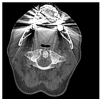
Figure 2.2: Three different nodal levels on an axial slice from a head and neck CT scan

Figure 2.3: Metal streak artifacts in a head and neck CT image

spread from different tumor sites. Figure 2.2 illustrates the distribution of some of the levels on a given CT slice. Drawing these nodal levels on each slice according to the official rules [15] is very difficult, because understanding the lymph regions depends on using its relationship to a variety of neighboring objects. Thus, segmentation of the lymph regions requires the segmentation of at least twenty anatomic objects on each side; typically it is many more than that. Some of these objects are modeled and shown in fig. 2.4. Also shown, is the Level-III nodal region in the form of a block of charcoal-coloured voxels.

In the next section, we discuss the challenges associated with segmenting the head and neck CT images.

2.2 Segmentation of the Head and Neck

(30)

(a) Anterior view (b) Posterior view

Figure 2.4: Some of the segmented head and neck organs with the Level-III nodal region

neighboring objects; this can be seen in the axial slice in fig. 2.2 where the bones are easily identifiable, but all the other objects seem to have similar intensities. For any segmentation method utilizing image intensities, this could result in inaccurate segmentations.

Many patients who have head and neck cancer have metal fillings in their teeth. In a CT scan, fillings can create metal streak artifacts, such as those shown in fig. 2.3. This further de-grades the image quality and presents another challenge for intensity-based methods. Though there exist several methods to mitigate these artifacts, we do not have much information on whether the existing segmentation methods will succeed on the improved images. I do not have to remove these artifacts from any images as the method presented in this thesis is based only on geometry and not image intensities.

(31)

atlases since a single atlas may not give accurate segmentations in all cases. The user has to pick an atlas similar anatomy to the patient, a non-trivial task. Even so, their results frequently require the user to edit the final result because these methods perform poorly in the presence of little contrast between neighboring objects, image artifacts, and noise.

Model-based methods can perform more stably when the image quality is not good, but they need a good initial guess for the shape and position of the model.

(32)

Chapter 3 Background

In this chapter, I will present background material on m-reps, thin plate splines, fluid flow registration (warping), and steady-state heat flow that will be helpful in understanding the de-tailed discussion of the components of my method presented in later chapters. Discrete medial models (m-reps) can model anatomical objects well and provide an object-centric coordinate system, which is necessary for my correspondence-based warping method. Section 3.1 dis-cusses discrete medial models for slab-like objects. Section 3.2 presents some prior work on image registration. In my correspondence-preserving warping method for image registration, I solve the steady-state heat equation; section 3.3 presents some prior work done with heat flow and techniques for speedy convergence of the system.

3.1 M-reps

In this section, I will talk about m-reps for slab-shaped objects. M-reps, which are a spe-cialization of the Blum medial axis representation, model a population of objects and provide correspondence between different members of the population. They were originally designed for slab-shaped objects and are generalized to nearly tubular objects in chapter 4.

(33)

Figure 3.1: A medial atom. Figure 3.2: An m-rep model of the medial scalene muscle showing the grid of medial atoms. The atoms at the edges of the grid are special – they are coalesced from an ordinary atom and one that is on the edge of the con-tinuous medial sheet.

vectors calledspokesthat end at and are approximately orthogonal to two implied boundary points. The hub and its two associated spokes are known as amedial atom. The medial atom,

mij, shown in fig. 3.1, is represented by the four-tuple(x, r,U−1,U+1), wherex∈R3 is the position of the hub, r ∈ _R+ _{is the common spoke length, and} _U−1_,_U+1 _∈

S2 are the two

spoke directions. These two spoke directions give us two opposing points on the surfaceb−1

andb+1_{, known as the} _{implied boundary points}_. _U−1 _and_U+1 _{are normal to the surface at} these points.

(34)

a rectangular mesh of medial atomsmij, wherei ∈ [1, m]andj ∈[1, n]. The curious reader is referred to Pizer et al. [29] for a much more detailed discussion on m-reps.

Section 3.1.1 presents the means to statistically analyze m-rep populations. This statistical analysis is useful in fitting m-reps to objects and provide correspondence across the popula-tion. Section 3.1.2 presents the mechanism in which m-rep models are fitted to anatomical objects. Finally, section 3.1.3 discusses the object-centric m-rep coordinate system, which is useful for my correspondence-based warping method.

3.1.1 M-rep Shape Space

As described in chapter 8 of the medial book [32], m-reps lie in aRiemannian symmetric shape space, where every point in this space is an m-rep. Moving along any smooth curve in this space yields a continuously varying m-rep model. Each point in this space is also associated with a tangent spaceTx(M)and a Riemannian metric, a smoothly varying inner product on this tangent space. Given a tangent plane, the operation that projects an m-rep model on this tangent plane is called alogarithmic map, and the operation that projects the model back to the shape space is called anexponential map.

(35)

3.1.2 M-rep Training

Training is the process of varying the parameters of the m-rep model so that the implied boundary and the expertly outlined boundary match each other.1 This process yields models with two desirable characteristics: First, they fit well – they match closely with the expertly outlined boundary; and second, they correspond well with models of other members of the population – the variation in parameters of the models across the population is low. This process, outlined in Merck et al. [26], is briefly presented in this section.

This process starts with the expert manually segmenting a few dozen training images. Sometimes, a set of landmarks is identified on the object; these are typically places on the object that can be easily identified across the entire population. Next, the parameters of the m-rep model are varied inside an optimizer that minimizes a weighted sum of the distances between the m-rep-implied boundary and the actual segmentation, the distances between the landmarks and the corresponding positions on the m-rep surface, and penalties due to bound-ary or medial surface roughness. The resulting models are calledtraining models.

These training models are then iteratively refined. Next, they are statistically analyzed: The modes of variation and a mean are computed. The fitting is repeated for each of the train-ing images by starttrain-ing with this mean model as the initial model and modifytrain-ing the model within the shape space to optimize the fit, possibly refining the result. This iterative pro-cess yields models that fit well (have a small average distance between the surface of the fitted model and the training image) and correspond well with models of other members of the population (have small standard deviations of the probability distribution of the model parameters).

1_{An accurate description of this method is parameter fitting, but I’ll call it training to be consistent with prior}

(36)

3.1.3 Figural Coordinates and Inter-object Correspondence

All points in the interior of a medially-implied object can be uniquely identified by a set of four coordinates: one running along the major dimension of the medial sheet, another running along the minor dimension, the third indicating the side of the medial sheet and enabling special handling at the edges, and the last one running from the medial sheet towards the surface. This coordinate system determines corresponding positions in the volume of two deformed versions of the model.

The m-rep mesh is considered to represent a continuous sheet of atoms with non-crossing spokes, which imply a closed figural boundary surface. This continuous sheet is obtained by interpolating the grid and is parameterized by(u, v)∈[(j, j+ 1)×(k, k+ 1)]for the part of the mesh with the atommjk at its lower left corner.

Methods for atom interpolation are described in Thall [35] and Han [17]; I use the method described by Thall. The result of this interpolation is that every surface point can be assigned a figural coordinate (u, v, φ). When φ is −π/2 or +π/2, it indicates the side. A value of

φ ∈ (−π/2,+π/2) indicates a position around the object’s crest, whose medial loci form the boundary of the medial grid. The parameters(u, v)are taken from the interpolated atom which corresponds to this surface point. The subdivision is done finely enough that the surface can be represented by a set of tiles with diameters less than the length of all sides of a voxel.

These coordinates can be extended to give unique, object-relative coordinates for the whole region interior to the implied boundary. For this purpose every point(x, y, z) in this region is assigned a figural coordinate(u, v, φ, τ), whereτ is a measure of distance from the hub along the spoke identified by(u, v, φ)as a fraction of the spoke lengthr. τ is0at the hub and1at the implied boundary.

(37)

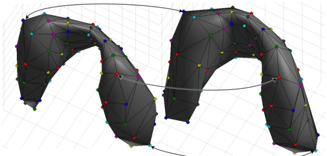
coordi-Figure 3.3: Correspondence between points on the surface of two different thyroids.

nates. Consider, for example, thyroids from two different patients. If an m-rep is fitted to one thyroid and then deformed to fit the second thyroid, then the corresponding positions on the two thyroids can be easily defined using this figural coordinate system. Fig 3.3 shows the correspondence for points on the surface of a thyroid. Thus, the m-reps and their figural coordinates provide a set of corresponding points.

It is important to refine these correspondences through the entropy-based correspondence step because these correspondences are only approximate. According to one school of thought, good correspondence is characterized by tighter probability distributions of the model param-eters. The correspondence inferred by m-reps suffers because they provide only approximate and large-scale fits to the object, and the fitting process is primarily geometric with very few image features.

3.2 Registration Methods

(38)

they match landmarks, image voxels, or a combination of both through a similarity metric. By regularizing the displacement or velocity field, these registrations yield a smooth spa-tial warp. Methods that regularize a displacement field typically do not produce diffeomor-phisms, which are one-to-one, smooth, and smoothly invertible mappings; methods that regu-larize velocity fields, however, most often produce diffeomorphisms.

Image-based registration techniques optimize a function that typically sums data mismatch and mapping irregularity terms. If the data mismatch term includes landmark mismatch, the optimizer will regularize the warp and match the image at the expense of the landmark match. Registration methods that constrain landmarks to match exactly include thin plate splines. Unfortunately thin-plate-spline-based methods do not guarantee diffeomorphisms.

The method of thin plate splines, developed by Bookstein et al. [3], is one of the pop-ular methods that matches landmarks and regpop-ularizes displacements; it is discussed in sec-tion 3.2.1. It is an important part of another registrasec-tion method discussed in secsec-tion 3.2.2, which matches landmark features and regularizes velocity fields; this method comes close to solving the issue of producing correspondence-preserving warps and is therefore of interest here. Of the methods that match image features and regularize velocity fields, the most popu-lar is fluid flow, developed by Joshi et al. [23]; I will not discuss fluid flow as our images have poor image intensity information and therefore fluid flow is not well suited.

3.2.1 Thin Plate Splines

Given a set of landmark pointsPi, each with a directional displacementhi, the thin plate spline

f(x) produces a smooth interpolation of the surface which passes through these landmark points.

(39)

flat on thex, y plane subjected to a small deformationf(x, y)in thez-direction. The elastic energy or the bending energyE stored in such a configuration is given by

ZZ R2  

∂2f ∂x2 2 + 2

∂2f ∂x∂y 2 +

∂2f ∂y2 2

 dxdy. (3.1)

If the steel plate is subjected to a fixed displacement at certain points, i.e., the landmarksPi, the rest of the plate takes a form such that this bending energy is minimized. Thus, thin plate splines yield the quadratically smoothest possible displacements.

In order to produce a mapping in three dimensions, instead of considering the displacement to be scalar-valued and perpendicular to the ‘3D plate’, consider it to lie within its ‘plane’. Thus, we now have a vector-valued displacement functionf(x, y, z) = (fx(x, y, z), fy(x, y, z),

fz(x, y, z))at each point(x, y, z)on the plate. The displacement field induced by this function is represented in the following form:

(x, y, z)→(fx(x, y, z), fy(x, y, z), fz(x, y, z)). (3.2)

In thin plate splines, this displacement field minimizes the Frobenius norm of each offx, fy, andfz.

Applying this idea of displacements to a 3D image, the new warped image is given by

Iwarped(x, y, z) = I(x+fx(x, y, z), y+fy(x, y, z), z+fz(x, y, z)). (3.3)

(40)

Figure 3.4: A 2D slice from a 3D CT scan in the application of thin plate spline reg-istration between two different patients: The level III lymph levels carried over in the registration are drawn in green. Notice that they are folded.

3.2.2 Large Deformation Diffeomorphisms

As just stated, a major problem of the thin plate spline registration method is that it does not necessarily generate a diffeomorphism. (Other spline methods also suffer from the same problem.) When the deformations between the atlas and the image under analysis are large and curved, the transformations introduce folding and do not preserve the topology of the atlas. The diffeomorphic landmark mapping framework developed by Joshi and Miller [23] can overcome this.

This framework defines a time-indexed transformation h(x, t) mapping the atlas to the target by integrating a velocity vector field:

h(x, t) = x+

Z t

0

v(h(x, t), t) dt. (3.4)

(41)

of a velocity field, the diffeomorphic transformation is given by the velocity vector field from the minimization:

ˆ

v(x, t) = arg min

v

Z 1

0

||Lv(x, t)||2_d_t subject to:v(h(xi, t)) =

dh(xi, t)

dt . (3.5)

Many linear differential operators have been used in the literature; the biharmonic thin plate spline (TPS) operator is the most common because it has a closed-form solution. Given the complete space-time paths of the landmark points, the closed-form solution for the velocity fields is given as a combination of an affine motion Ax+T and a weighted superposition of Green’s functions of the differential operator LL†, where L† is the adjoint of the linear differential operatorL, with weightsβi(t):

v(x, t) =

N

X

i=1

βi(t)K(h(xi, t),x) +Ax+T. (3.6)

The weightsβi(t)and the affine motionAx+T are chosen so that the velocity field satisfies the set of constraintsv(h(xi, t)) = dh(xi, t)/dt and any additional boundary conditions. In three dimensions, using the TPS operator with zero boundary condition at infinity results in a Green’s functionK(x,y)given by1/|x−y|and the conditions

N

X

i=1

βi(t) = 0 and N

X

i=1

βi(t)h(xi) = 0.

(42)

Discrete Integration of Velocity Fields.

For a practical computer implementation the continuous integral of the velocity vector fields is discretized in time as follows: Lettj, j = 0,· · · , M be a discretization of the interval[0,1]; then, given a velocity fieldv(x, t), the integral in equation 3.4 can be written recursively as

h(x, tj+1) = h(x, tj) +

Z tj+1 tj

v(h(x, t), t) dt

with tj =

j

M, j = 0,· · · , M.

The integral above is approximated, resulting in

h(x, tj+1) = h(x, tj) +

1

Mv(h(x, tj), tj), (3.7)

with the initial condition h(x,0) = x. Using this discretization, the generation of a large deformation diffeomorphic transformation can be seen as a repeated application of a TPS interpolation. Substituting equation 3.6 into equation 3.7 yields a solution of a sequence of thin plate spline problems:

h(x, tj+1)−h(x, tj)

1/M =

N

X

i=1

(βi(tt)K(h(xi, tj),x) +Ajx+Tj). (3.8)

This can be interpreted as a repeated application of a spline interpolation for incremental small motions of the landmark along the given paths.

(43)

3.3 Steady-state Heat Flow

Is a diffeomorphism really what we want? It may be too restrictive and a smooth, non-folding warp would suffice. My method constructs a steady-state heat flow problem whose solution yields the necessary landmark-matching smooth, non-folding warp. Heat flow was first used by Jones et al. [22] to compute cortical thickness. Yezzi et al. [37] improved the method and used it to compute tissue thickness. Dinh et al. [12] interpolated 3D objects by solving a heat flow equation. The steady-state heat flow partial differential equation takes the form of Laplace’s equation. Section 3.3.1 presents a little background on the Laplace’s equation, and section 3.3.2 talks about techniques to solve this equation.

3.3.1 Laplace’s Equation

Laplace’s equation is widely used in physics to solve gravitational, electrodynamic, thermo-dynamic, fluid flow, and other systems. It is a second-order partial differential equation of a scalar fieldφ, written using the Laplacian operator∆:

∆φ = ∂

2_φ

∂x2 +

∂2φ ∂y2 +

∂2φ

∂z2 = 0. (3.9)

This equation is typically accompanied by a fixed value for the scalar field on some bound-aries. Solutions of this equation are calledharmonic functionsin mathematics andpotential functionsin physics.

(44)

Equi-potential surfaces

Streamlines Boundaries

Figure 3.5: Solution of Laplace’s equation: The top and bottom curves are fixed value bound-ary surfaces. Solid lines indicate equi-potential lines, and dotted lines show the streamlines.

Laplace’s equation is an elliptic partial differential equation. A useful property of an elliptic PDE is that the solution is necessarily smooth – in the case of Laplace’s equation, two orders smoother than the boundary conditions.

3.3.2 Solving Laplace’s Equation

For simplicity, consider the solution of Laplace’s equation in two dimensions. The numerical methods in two dimensions are the same as in three dimensions.

The 2D Laplace’s equation, whereφis the temperature at a point in space, is given by

∆φ= ∂

2_φ

∂x2 +

∂2_φ

∂y2 = 0. (3.10)

(45)

the spacing of the grid, is given by

φi+1,j+φi−1,j+φi,j+1+φi,j−1−4φi,j

h2 = 0. (3.11)

Such an equation is typically solved by a relaxation method such as Jacobi iterations:

φt+1_i,j = φ

t

i+1,j+φti−1,j+φti,j+1+φti,j−1

4 , (3.12)

whereφt_i,j is the value of the temperature at location(i, j)in iterationt.

Jacobi iterations can run in parallel but take a lot of time to converge. This is improved by two methods called red-black ordering and Successive Overrelaxation (SOR).

The method of red-black ordering exploits the fact that the value of a new iterate is only dependent on its four non-diagonal neighbors (in two dimensions). Imagine the entire location grid as a chessboard (with red and black colors); the value at the red squares is dependent only on its black neighbors and vice-versa. Thus, one could update all red positions in parallel and then all black positions in parallel.

φt+1_i,j = φ

t

i+1,j+φti−1,j+φti,j+1+φti,j−1

4 ∀ red points(i, j), (3.13)

φt+1_i,j = φ

t+1 i+1,j+φ

t+1 i−1,j+φ

t+1 i,j+1+φ

t+1 i,j−1

4 ∀ black points(i, j). (3.14)

By itself, red-black ordering increases the convergence speed only by a factor of two. The second improvement, which requires red-black ordering, is calledSuccessive Overrelaxation (SOR). In Jacobi iterations, the value is relaxed by a factor of 1. In SOR, the iterates are ‘over-relaxed’ by a factor ofω, the Chebyshev acceleration. For an optimum value ofω, the iterations converge extremely fast. The new update equations are given by

φt+1_i,j = φt_i,j+ω× φ t

i+1,j+φti−1,j+φti,j+1+φti,j−1−4φti,j

4

!

(46)

φt+1_i,j = φt_i,j+ω× φ t+1 i+1,j+φ

t+1 i−1,j+φ

t+1 i,j+1+φ

t+1

i,j−1−4φti,j

4

!

∀ black points(i, j). (3.16)

(47)

Chapter 4 Quasi-tubular Medial Models

4.1 Introduction

In the human body, the blood vessels, the bronchi, and the colon are examples of nearly tubu-lar objects. Segmenting these objects is an important task in medical imaging, and learning probability distributions on their populations is useful to segmentation algorithms [6]. Repre-senting these objects with slab-shaped m-reps, as shown in fig. 4.1 is unstable. However, most of them can be represented as a tube at the large scale with smaller scale changes understood as deviations from the tube. Some of these are shown in fig. 4.2.

A good statistical model for a population of objects consists of good geometric and image intensity representations. A good geometric model should stably and uniquely represent a population of objects and not just a single member, and it should provide correspondence between different members of the population. A good image intensity model should be able to represent image intensity distributions around the object for a good-quality segmentation. All these criteria are satisfied by the quasi-tubular medial models developed in this chapter along with the image intensity distribution model developed by Broadhurst [4] and Stough [33].

(48)

Medial surface Object boundary

Figure 4.1: A cross-section through a nearly tubular object. As the cross-section marginally changes, the orientation of the medial surface changes by90◦depicting the instability in rep-resenting a nearly tubular object with a slab-shaped m-rep.

Figure 4.2: Renderings of quasi-tube models fitted to different objects. From the left to right the objects are sections of the head and neck’s skin surface extracted from a 3D CT scan, the carotid artery, the internal jugular vein, and a section of the upper airway.

of a good statistical model. I then discuss my representation of a tube and representation of a population of tubular objects, and I see how these representations perform in practice.

The first part of a good statistical model for tubes is its geometric representation. There are several tubular models discussed in the literature. They fall into three broad categories – medial, skeletal, and boundary representations. The medial tubular model, defined by Koen-derink [25], is the envelope of a set of spheres centered on a space curve. Skeletal tubular models include swept surfaces and generalized cylinders. Boundary representations will not be discussed here because they are not specific to tubular objects.

(49)

curve – a one-dimensional (1D) curve along which a cross-section is swept to generate a volume. The several definitions of a generalized cylinder differ in restrictions on the skeletal curve and on the section function. A tubular generalized cylinder has a circular cross-section that may vary in size and have a bent skeletal curve. A point on a medial curve has an entire curve on the boundary equidistant from it, whereas a point on a skeletal curve can be much closer to one side than the other.

The second part of a good statistical model is the representation of image intensity patterns around objects of a population. 3D CT images of the human body and the head and neck in particular often have poor contrast between soft tissue objects. This increases the signal-to-noise ratio and adversely affects the stability of a segmentation method that uses image intensities from a small region. For example, the physically motivated model by Terzopoulos et al. [34] uses image intensity forces that may not behave stably in the presence of poor contrast. A more stable approach would be to acquire image intensities over several large regions spread around the object of interest.

Segmentations can be stabilized in the presence of poor intensities by limiting the defor-mation to credible shapes. Doing so requires the knowledge of the different shapes the object can possibly take. Statistics is a suitable way to characterize these variations in shape and intensities. Our group has employed a statistical method of modeling intensities, developed by Broadhurst [4] and Stough [33], that leads to a more stable segmentation process in the presence of poor contrast and noise.

(50)

4.1.1 Prior Work on Modeling Tubular Objects

There are several definitions associated with center-line-based tubular models. The definitions and the methods that implement them differ by whether the center-line and cross-sections are restricted, whether the center-line is unique, and whether the method is robust with respect to the number of training samples. Several of these definitions and their shortcomings are presented in the next few paragraphs.

Generalized cylinders, also known as generalized cones, were fist proposed by Binford [2] with special instances studied extensively in computer vision. A straight homogenous gen-eralized cone [36] is the surface obtained by sweeping a fixed cross-section along a straight line while possibly scaling it, whereas a straight homogenous generalized cylinder may have a cross-section that can change shape. Huang et al. [20, 19] discuss generalized tubes, which are constructed by sweeping a fixed cross-section along a curve with certain constraints.

Several center-line-based methods do not generate unique center-lines. To model popula-tions, however, there must be a unique center-line found in a principled manner, so that varia-tion introduced by the modeling process is not reflected in the statistics. O’Donnell et al. [27] discuss a novel method of generalized cylinders that works around part of this uniqueness problem by starting with a base cross-section that may be anisotropically scaled. Although they use only two scaling parameters, their method can be extended to produce arbitrary scal-ing. Further, they allow for local deformations of the cross-section by a spline function on the surface. Terzopoulos et al.’s [34] deformable model, which uses image-based and regularity forces to deform the model, can represent a wide range of tubular objects. However, none of them have discussed any means to compute statistics of their objects. It is also not trivial to extend any of them to include a statistical representation of the object they are modeling.

(51)

of the centers of swept spheres.) Sweeping a non-circular cross-section typically results in a 2D medial surface. When the medial surface degenerates to a curve, we call it amedial axis. Having a true medial axis representation overcomes the issue of finding a unique center-line. The class of generalized cylinders whose medial axis is a curve is restricted to those with a circular cross-section.

A generalized cylinder and an object with a well-defined medial axis are closely related. When we sweep a constant circular cross-section along an appropriately smooth curve, the curve forms the medial axis of the generated surface. However, if we sweep a non-constant circular cross-section along a curve, the generated object may not have a curve as its medial locus though some such objects (generated by sweeping spheres of varying sizes) will have a curve as the medial locus. Even when a generalized cylinder does not have a curve as its medial axis, it is useful to find an approximate medial axis for that object because the orientation of the medial surface across a population can be unstable.

Not all combinations of cross-sections and curves form a legal generalized cylinder. A sweep of a cross-section along a curve may result in two adjacent cross-sections crossing each other near a sharp bend on the curve. Such instances of the generalized cylinder are illegal, restricting the range of permissible cross-sections and medial curves. Damon [8] has described a method in the swept surface paradigm using a shape operator that can be used to detect these illegal generalized cylinders.

Finally, a quasi-tubular object can be thought of as an object that is modeled as deviations from a tubular object. In the general case, it is an object with a star-shaped1_{cross-section that} may not be close to circular but varies slowly along the medial axis.

No specialized means of performing statistics has been developed for the generalized cylinders and swept surface models discussed above; they are best suited for modeling in-dividual quasi-tubular objects and not populationsof them. Because statistical descriptions

1_{A star-shape is one where there exists a point in the interior of the shape such that every line connecting a}

(52)

can stabilize segmentations, there has been some work on statistically modeling tubes. One of the methods, called generalized stochastic tubes, developed by Huang et al. [21], aids in the segmentation of blood vessels but is specialized for this application. Another method, developed by de Bruijne et al. [10], retrofits Active Shape Models with center-lines but lacks a robust image appearance model.

(53)

the objects is related to the surface curvatures: The curvature of the surface in blood vessels changes slowly along the circumferential direction and stays almost the same as that of the medial curve in the axial direction. In rectums and other objects, the surface curvature is not related closely to the medial curvature.

4.1.2 The Driving Problem: Segmentation of Quasi-tubes

The method of segmentation via posterior optimization of m-reps, developed by Pizer et al. [29], has been successful in dealing with slab-shaped objects with a lot of variability and poor contrast. We develop a new method that draws on the strengths and ideas from these methods but represents a tube-like object with a discretely sampled medial space curve and then models quasi-tubes as deviations from these tubes.

The segmentation method can be divided into two parts – training and the actual segmen-tation itself. During training, a rough m-rep model of the object is allowed to vary inside an optimizer that favors smooth models with a regularly spaced discrete medial mesh and that match well with the image data. The resulting models are known as training or fitted models. Next, these training models are statistically analyzed. The variation in the shape space of the models is studied using Principal Geodesic Analysis (PGA), developed by Fletcher et al. [13], which is a form of Principal Component Analysis (PCA) suited for non-linear spaces. The result is a mean shapemand a priorp(m)for segmentation. At the same time, the region around the object is divided into small parts, and the distribution of intensities in each region is studied with the help of local region intensity quantile functions, developed by Broadhurst [4] and Stough [33]. We then apply PCA on these quantile functions to produce a likelihood functionp(I|m)for segmentation.

(54)

logp(I|m) with the weights chosen to make the two terms have equal variance. This is a variant of the method of posterior optimization.

Similarly, for quasi-tubes we start with a tubular medial model that during training is de-formed to a quasi-tubular model. Shape and intensity statistics are obtained, and then these probability distributions are used to drive the segmentation. As with slabs, the objective func-tion isw1logp(m) +w2logp(I|m).

The remainder of the chapter is organized as follows: Section 4.2 describes the represen-tation and geometry of tubular medial models. Section 4.3 describes the way in which we estimate probability distributions on these models. Section 4.4 presents a study on the per-formance of the tube model in simulated rectums. Section 4.5 details the modeling of the deviations from a tubular to a quasi-tubular model. Section 4.6 gives more details of the train-ing and segmentation approaches. Finally, section 4.7 presents quantitative and qualitative results obtained by applying my method on real data obtained from CTs of rectums.

4.2 Medial Models for Tubes

This section describes the representation and geometry of tubular medial models. The struc-ture of a tubular m-rep is described in the following manner: A first order tube m-rep is a continuous space curve with a cone placed at every point along the curve. The axis of the cone is tangential to the space curve at the tip of the cone. Sweeping the edges of the cone bases gives the boundary of the modeled object, which is orthogonal to the rays from the cone tip to the cone base. The cones may have a half cone angle greater thanπ/2but less thanπ. They are not allowed to intersect each other. Damon [7] has provided us with tools that can be used to measure local self-intersection (folding) of the object implied by the medial surface of a slab m-rep. In section 4.2.1 we adapt these tools to do the same for tubular m-reps.

Atlas diffeomorphisms via object models