P. Van Isacker,1 J. Engel,2 and K. Nomura1, 3, 4 1
Grand Acc´el´erateur National d’Ions Lourds, CEA/DRF-CNRS/IN2P3, Bvd Henri Becquerel, F-14076 Caen, France
2Department of Physics and Astronomy, University of North Carolina, Chapel Hill, NC, 27516-3255, USA 3
Physics Department, Faculty of Science, University of Zagreb, HR-10000 Zagreb, Croatia
4
Center for Computational Sciences, University of Tsukuba, Tsukuba 305-8577, Japan (Dated: November 6, 2018)
Background: The interacting boson model has been used extensively to calculate the matrix
ele-ments governing neutrinoless double-beta decay. Studies within other models—the shell model, the quasiparticle random-phase approximation, and nuclear energy-density functional theory—indicate that a good description of neutron-proton pairing is essential for accurate calculations of those ma-trix elements. The usual interacting boson model is based only on like-particle pairs, however, and the extent to which it captures neutron-proton pairing is not clear.
Purpose: To determine whether proton pairing should be explicitly included as
neutron-proton bosons in interacting-boson-model calculations of neutrinoless double-beta decay matrix elements.
Method: An isospin-invariant version of the nucleon-pair shell model is applied to carry out
shell-model calculations in a large space and in a collective subspace, and to define effective operators in the latter. A democratic mapping is then used to define corresponding boson operators for the interacting boson model, with and without an isoscalar neutron-proton pair boson.
Results: Interacting-boson-model calculations with and without the isoscalar boson are carried out
for nuclei near the beginning of thepfshell, with a realistic shell-model Hamiltonian and neutrinoless double-beta-decay operator as the starting point. Energy spectra and double-beta matrix elements are compared to those obtained in the underlying shell model.
Conclusions: The isoscalar boson is not important for energy spectra but improves the results
for the double-beta matrix elements. To be useful at the level of precision we need, the mapping procedure must be further developed to better determine the dependence of the boson Hamiltonian and decay operator on particle number and isospin. But the benefits provided by the isoscalar boson suggest that through an appropriate combination of mappings and fitting, it would make interacting-boson-model matrix elements more accurate for the heavier nuclei used in experiments.
PACS numbers: 21.60.Cs, 21.60.Ev,21.30.Fe
I. INTRODUCTION
Experiments to measure the rate of neutrinoless double-beta (0νββ) decay, in which two neutrons decay to two protons and two electrons, are growing in number and expense [1–4]. A nonzero rate would imply that neu-trinos are Majorana particles [5] and provide information about neutrino masses [6, 7], and possibly about exotic new particles [8]. To efficiently plan and interpret the experiments, however, one must know with reasonable accuracy the nuclear matrix elements that govern the decay. The matrix elements cannot be measured, and so calculating them with controlled precision has become an important theoretical goal.
A variety of many-body methods have been loosed on the matrix element problem [9]. Of these, most are em-bedded in phenomenological models that describe energy levels and other decay processes well in heavy nuclei. The interacting boson model (IBM) [10], in which the funda-mental constituents are spin-zero and spin-two bosons that stand both for like-nucleon pairs and the collective quadrupole degree of freedom, is a good example [11– 13]. The version called IBM-2 [14], in which neutron and proton bosons are distinguishable, successfully describes spectra and electromagnetic transitions [10] plus single-β
decay [15] in a wide variety of nuclei.
Because the IBM is equivalent to the Bohr-Mottelson collective model in certain limits, one might expect the important physics in the IBM to mirror that in approaches such as nuclear energy-density functional (EDF) theory, in which quadrupole degrees of freedom are emphasized. Similarly, because the IBM’s bosons are related to collective shell-model excitations, the impor-tant physics in the IBM and the shell model should have something in common. In both EDF-based methods—in particular, the generator coordinate method (GCM)— and in the shell model, 0νββ matrix elements tend to be too large unless care is taken with theJ = 1, T = 0 (isoscalar) pairing interaction. That component of the nuclear Hamiltonian has been known to be important from QRPA calculations [16, 17] for nearly 30 years. More recently, Ref. [18] showed that the inclusion of the isoscalar-pairing amplitude as a generator coordinate re-duces matrix elements significantly, and Ref. [19] showed that the isoscalar pairing in the Hamiltonian does the same in the shell model. Here we investigate whether it plays a similar role in the IBM. More explicitly, we ask whether we need to add a spin-1 isoscalar boson to the model to avoid over-estimating 0νββ matrix elements, and try to provide an answer.
To address the question, one would like to modify the IBM 0νββ calculations of Refs. [11–13] by adding the isoscalar spin-1 boson, which we will label p. But be-cause the IBM Hamiltonian is phenomenological, we do not knowa priorihow to add to and alter its Hamiltonian so as to correctly include the physics of the new boson. One might examine single-βdecay and other processes in which the boson could play a significant role in order to pin down new terms in the Hamiltonian, but that task is beyond what we are able to do here. Instead, we try to derive the boson Hamiltonian and the corresponding decay operator, not in nuclei that actually undergo 0νββ
decay, but rather in lightpf-shell nuclei for which exact shell model results are available, both for spectra and for 0νββ matrix elements [19]. Since the IBM is supposed to represent collective dynamics in a major shell, we con-struct a mapping of operators from thepf shell to a set of bosons, including not only the usual bosons of the IBM-2 but “neutron-proton” bosons as well. Ref. [11] developed a mapping to obtain a boson 0νββoperator; here, start-ing from square one, we map the Hamiltonian as well. Though this procedure will not tell us how much ap bo-son would change the realistic IBM 0νββ predictions, it will give us a good idea of the extent to which apboson is required to faithfully reflect shell-model results.
It is not obvious that the extra boson will improve the description of 0νββ decay. Certainly it will cap-ture some of the isoscalar-pair correlations that elude the IBM-2. But because the product of two isoscalarJ = 1 pair creation operators can be rewritten as a superpo-sition of products of proton pair creation operators and neutron pair creation operators, some of the physics of isoscalar pairing is probably already in the IBM-2. Fur-thermore, the use of too many boson types can cause a model to degrade for a related reason: an over-counting, roughly speaking, of the independent collective degrees of
freedom. Thus, though an independent isoscalar-pairing coordinate is clearly important in GCM calculations of 0νββ matrix elements, an isoscalar boson may or may not improve the corresponding IBM calculations.
We carry out the mapping from shell model to IBM in two steps, the first of which relies on the nucleon-pair shell model (NPSM) [20–22] to define a collective subspace. We briefly review the NPSM in Secs. II and III, with the main purpose of introducing notation for an isospin-invariant formulation of the model [23]; with a collective subspace specified by the NPSM, we show in Sec. IV that we can use the method of Suzuki and Lee [24] to construct effective operators for the subspace. The second step, which we describe in Sec. V, involves the mapping of the (effective) Hamiltonian and the 0νββ -decay operator from the fermion to boson spaces. In Sec. VI we apply the formalism to the energy spectra of and 0νββ-transition strengths between nuclei in the lower part of thepfshell, taking into account correlations in the entire shell. Finally, in Sec. VII, we present our conclusions.
II. THE NUCLEON-PAIR SHELL MODEL
We introduce the following notation for pairs of fermions:
Pα†ΓM
Γ ≡(a †
γ1×a †
γ2) (Γ)
MΓ, (1)
whereγi denotes the angular momentum ji and isospin
ti (which is always 12) of a single nucleon, Γ stands for
the coupled angular momentumJ and isospinT (which can be 0 or 1) of the nucleons with γ1 and γ2 (with α standing forγ1, γ2), andMΓrepresents the corresponding projections (i.e.,MΓ =MJMT). We write an arbitrary
n-pair state of the NPSM as
|α1Γ1. . . αnΓnΛ2. . .Λni ≡ · · ·
Pα†
1Γ1×P †
α2Γ2
(Λ2)
×Pα†
3Γ3
(Λ3)
× · · · ×Pα†
nΓn
!(Λn)
|Oi, (2)
or,
|Pri ≡ |α1Γ1. . . αnΓnΛ2. . .Λni, r= 1, . . . ,Θ, (3)
for short. The state |Oi in Eq. (2) is the bare fermion vacuum, and the indexrin Eq. (3) stands for the set of quantum numbers{α1Γ1. . . αnΓnΛ2. . .Λn}, which
spec-ifies the character of then pairsαqΓq, the set Λq of
in-termediate angular momenta and isospins, and Λn, the
state’s total angular momentum and isospin.
In general the basis in Eq. (2) is non-orthonormal and overcomplete. A calculation in this basis therefore re-quires the diagonalization of the overlap matrixhPr|Psi, the elements of which can be computed with a recur-rence relation presented in Ref. [21] and generalized to
include isospin in Ref. [23]. Here we need matrix ele-ments between one- and two-pair states; these are trivial for n = 1 and summarized in Appendix A for n = 2. Vanishing eigenvalues of the matrixhPr|Psiindicate the
overcompleteness of the pair basis. In a subspace of Ω pair states in which all eigenvalues of the overlap matrix are non-zero, one can construct an orthonormal set given by:
|P¯ri=
r
1
Or
Ω
X
s=1
Crs|Psi ≡
Ω
X
s=1 ¯
Crs|Psi, r= 1, . . . ,Ω,
whereOris thertheigenvalue of the Ω×Ω overlap matrix:
Ors≡ hPr|Psi, r, s= 1, . . . ,Ω, (5)
and the coefficients{Crs, s= 1, . . . ,Ω}specify the
corre-sponding eigenvector. If Ω is the dimension of the original shell-model spaceH, which we call the “complete”
shell-model space, then the vectors{|Pr¯ i, r= 1, . . . ,Ω} form a basis ofH.
It is important to distinguish between the total number Θ of possiblen-pair states in Eq. (3) and the number Ω≤
Θ of linearly independent states among them. To apply the NPSM in a collective subspace, one needs to expand an arbitraryn-pair state in terms of the orthogonal basis states,
|Pri= Ω
X
s=1
Ars|Ps¯ i, r= 1, . . . ,Θ, (6)
where the coefficientsArsare given by
Ars≡ hPr|Ps¯ i= Ω
X
t=1 ¯
CsthPr|Pti, (7)
with r = 1, . . . ,Θ and s = 1, . . . ,Ω. We assume here
and henceforth that the matrix elements are real, that is, thathPr|Psi=hPs|PriandhP¯r|Psi=hPs|P¯ri.
An arbitrary shell-model operator ˆTf (where f stands for “fermion”) between two sets of orthogonal basis states,
|P¯r00i=
Ω0
X
s0=1 ¯
Cr00s0|Ps00i, r0= 1, . . . ,Ω0,
|Pr0000i=
Ω00
X
s00=1 ¯
Cr0000s00|Ps0000i, r00= 1, . . . ,Ω00, (8)
has the matrix elements
hP¯r00|Tˆf|P¯r0000i=
Ω0
X
s0=1
Ω00
X
s00=1 ¯
Cr00s0C¯r0000s00hPs00|Tˆf|Ps0000i
= ( ¯CCC0×TTTf×CCC¯00T)r0r00.
(9)
HereMMMT is the transposed matrix ofMMM and ¯CCC0,TTTf, and ¯
C
CC00 are the following matrices: ¯
CCC0:{C¯r00s0, r0= 1, . . . ,Ω0, s0= 1, . . . ,Ω0},
TTTf:{hPs00|Tˆf|Ps0000i, s0= 1, . . . ,Ω0, s00= 1, . . . ,Ω00}, ¯
C
CC00:{C¯r0000s00, r00= 1, . . . ,Ω00, s00= 1, . . . ,Ω00}.
(10)
For the Hamiltonian operator, ˆTf = ˆHf, the dimen-sions in bra and ket of Eq. (9) are the same, Ω0= Ω00≡Ω, and the diagonalization of the Ω×Ω Hamiltonian matrix leads to the eigenstates
|Et¯ i= Ω
X
r=1
Etr|Pr¯ i, t= 1, . . . ,Ω, (11)
where the coefficients{Etr, r= 1, . . . ,Ω}are the compo-nents of the eigenvector associated with the eigenvalue
Et. If ˆTf is another operator, e.g. a transition operator,
its action on eigenstates of ˆHf in the complete Hilbert spaceHis given by
hE¯0t0|Tˆf|E¯t0000i=
Ω0
X
r0=1
Ω00
X
r00=1
Et00r0Et0000r00hP¯r00|Tˆf|P¯r0000i
= (EEE0×CCC¯0×TTTf×CCC¯00T ×EEE00T)t0t00, (12)
witht0= 1, . . . ,Ω0 andt00= 1, . . . ,Ω00.
All this shows us that it is possible to carry out stan-dard shell-model calculations in the NPSM, albeit in a complicated way. The advantage of the NPSM is that it allows a truncation to a shell-model subspace constructed in terms of collective pairs.
III. COLLECTIVE SUBSPACE
A collective fermion pair is a superposition of pairs built from orbits with differentγ1 andγ2, all coupled to the same Γ. It can be specified by its coefficientsαΓγ1γ2:
B†αΓM
Γ ≡
X
γ1γ2
αΓγ
1γ2(a †
γ1×a †
γ2) (Γ)
MΓ, (13)
where the subscriptαis to emphasize the dependence of the pair on its coefficients. After selecting a particular set of collective pairs{BΓ}, we can construct NPSM states from them,viz.
|α1Γ1. . . αnΓnΛ2. . .Λni ≡ · · ·
B†α
1Γ1×B †
α2Γ2
(Λ2)
×Bα†
3Γ3
(Λ3)
× · · · ×Bα†
nΓn
!(Λn)
|Oi. (14)
Although the formalism does not require it, we shall henceforth consider only one collective pair for a given
{Γ1. . .ΓnΛ2. . .Λn} and leading to the abbreviation |Bii ≡ |Γ1. . .ΓnΛ2. . .Λni, i= 1, . . . , ω , (15)
whereω is the number of couplings{Γ1. . .ΓnΛ2. . .Λn}.
The collective NPSM states in Eq. (14) can be ex-pressed as linear combinations of the non-collective ones in Eq. (2):
|Bii=
Θ
X
r=1
air|Pri=
Θ X r=1 Ω X s=1
airArs|P¯si
= Ω
X
s=1
(aaa×AAA)is|Ps¯ i, i= 1, . . . , ω ,
(16)
with coefficientsair that are functions ofαΓγ1γ2. Results analogous to those in Sec. II can now be obtained by diagonalizing the collective overlap matrix
oij≡ hBi|Bji=
Ω
X
r=1
(aaa×AAA)ir(aaa×AAA)jr
= (aaa×AAA×AAAT×aaaT)ij, i, j= 1, . . . , ω .
(17)
The number of linearly independent vectors|Biiis given by the number of non-zero eigenvalues of the matrixoij.
We assume here that all eigenvalues of the matrix (17) are non-zero, which will be the case for any reasonable choice of the collective subspace. As we have noted, the NPSM is interesting because when one restricts oneself to a set of collective pairs, the resulting space has a much lower dimension than doesHitself,i.e.,ωΩ.
To carry out a shell-model calculation in the collec-tive subspace, we employ notation that is analogous to what we used for the full spaceH. Thus, we work with
orthonormal states
|Bi¯ i=
r 1 oi ω X j=1
cij|Bji ≡
ω
X
j=1 ¯
cij|Bji
= Ω
X
r=1
(¯ccc×aaa×AAA)ir|P¯ri ≡
Ω
X
r=1
bir|P¯ri,
(18)
whereoi is theith eigenvalue of the overlap matrix (i=
1, . . . , ω) and the coefficients{cij, j= 1, . . . , ω}make up
the corresponding eigenvector. A shell-model operator ˆ
Tf has the matrix elements
hB¯i00|Tˆf|B¯i0000i=
Ω0
X
r0=1
Ω00
X
r00=1
bi0r0bi00r00hP¯r00|Tˆf|P¯r0000i
= (bbb0×CCC¯0×TTTf×CCC¯00T×bbb00T)i0i00, (19)
withi0 = 1, . . . , ω0 and i00= 1, . . . , ω00. For the Hamilto-nian operator, ˆTf = ˆHf, the matrix (19) has dimension
ω×ω and its diagonalization leads to the eigenstates
|¯eki=
ω
X
i=1
eki|Bi¯i= Ω
X
r=1
(eee×bbb)kr|Pr¯ i, (20)
with k = 1, . . . , ω and with the coefficients {eki, i =
1, . . . , ω}given by the components of the eigenvector
as-sociated with the eigenvalueek. If ˆTf is some other
op-erator, its matrix elements in the basis of eigenstates of ˆ
Hf are given by
h¯e0k0|Tˆf|¯ek0000i= (eee0×bbb0×CCC¯ 0
×TTTf×CCC¯00T×bbb00T×eee00T)k0k00, (21) withk0= 1, . . . , ω0 andk00= 1, . . . , ω00.
IV. EFFECTIVE SHELL-MODEL OPERATORS
IN A COLLECTIVE SUBSPACE
The eigenspectrum of ˆHf and the matrix elements of transition operators ˆTf in the restricted Hilbert space differ from the corresponding eigenspectrum and matrix elements of the operators in the complete Hilbert space
H. We need an effective Hamiltonian ˆHefff and, more generally, effective operators ˆTefff in the restricted Hilbert space that preserve the original eigenvalues and matrix elements. We begin their construction by lettingHP be
the restricted Hilbert space andHQ the excluded Hilbert
space, with H = HP ∪HQ. The operators ˆP and ˆQ
project onto the corresponding spaces, so that ˆPH = HP and ˆQH = HQ. The eigenstates of ˆHf in H are
given by{|E¯ti, t= 1, . . . ,Ω} and those of ˆHf in HP by {|e¯ki, k= 1, . . . , ω}. For each eigenstate|e¯kiwe identify
a corresponding eigenstate |Ek¯ i, usually by requiring a maximum overlap
hEk¯ |¯eki= Ω
X
r=1
Etr(eee×bbb)kr = (EEE×bbbT ×eeeT)tk. (22)
This procedure defines a set ofωeigenstates{|Et¯ki, k =
1, . . . , ω} and an associated ω×Ω matrix ˜EEE with the
elements ˜
E E
E:{Ekr˜ ≡Etkr, k= 1, . . . , ω, r= 1, . . . ,Ω}. (23)
For each of the eigenstates|Et¯ kiwe define its component inHP,
|eki ≡Pˆ|Et¯ki, k= 1, . . . , ω , (24)
and assume that the states {|eki, k = 1, . . . , ω} are lin-early independent and therefore span the entire restricted Hilbert spaceHP.
We use the method of Suzuki and Lee [24] to deter-mine effective operators inHP. The method employs an
operator ˆη that maps states in HP to states inHQ such
that
ˆ
η|eki= ˆQ|Et¯ki, k= 1, . . . , ω . (25)
Since ˆη= ˆQηˆPˆ, the operator ˆη satisfies the relations ˆ
It follows that
|Et¯ki= ( ˆP+ ˆQ)|Et¯ki=|eki+ ˆη|eki= ( ˆI+ ˆη)|eki, (27) and, inversely, that
|eki= ( ˆI−ηˆ)( ˆI+ ˆη)|eki= ( ˆI−ηˆ)|Et¯ki. (28) The transformed (non-hermitian) Hamiltonian ˆHf≡( ˆI− ˆ
η) ˆHf( ˆI+ ˆη) satisfies the relation ˆ
Hf|eki= ( ˆI−ηˆ) ˆHf|Et¯
ki=Etk( ˆI−ηˆ)|Et¯ki=Etk|eki, (29) which shows that the states {|eki, k = 1, . . . , ω} are
eigenstates of ˆHf, with eigenvalues{Et
k, k= 1, . . . , ω}. A matrix element of ˆηis nonzero only if the bra is inHQ
and the ket inHP. The operator is therefore determined
by the matrix elements
hPr¯ |ηˆ|Bi¯ i, r= 1, . . . ,Ω, i= 1, . . . , ω , (30) where |Pr¯ i ∈ H and |Bi¯ i ∈ HP. To calculate the
ma-trix elements in Eq. (30), we first note that although the states {|eki, k = 1, . . . , ω} span the entire Hilbert
spaceHP, they do not form an orthonormal basis. A
bi-orthogonal basis{hek˜ |, k= 1, . . . , ω}can be defined such that
he˜k|ek0i=δkk0, (31) which implies that the operator ˆP, which is nothing but the identity operator onHP, can be written as
ˆ
P =
ω
X
k=1
|eki hek˜ |. (32)
Thus we have
hPr¯ |ηˆ|Bi¯i=
ω
X
k=1
hPr¯|ηˆ|eki hek˜ |Bi¯ i. (33)
The first matrix element in this sum can be written as
hPr¯ |ηˆ|eki=hPr¯ |Et¯ki − ω
X
i=1
hPr¯ |Bi¯ i hBi¯ |Et¯ki, (34)
where we have used the relation ˆP =P
|B¯ii hB¯i|. With
the help of Eqs. (11) and (18) we deduce the relations
hPr¯ |Et¯ki= ˜Ekr, hPr¯ |Bi¯ i=bir, hBi¯|Et¯ki= (bbb×EEE˜T)ik,
(35) which lead to the following expression for the first matrix element in the sum in Eq. (33):
hPr¯ |ηˆ|eki= ˜Ekr−( ˜EEE×bbbT ×bbb)kr. (36)
To determine the second matrix element in the sum in Eq. (33), we note that
hB¯i|B¯ji= ω
X
k=1
hB¯i|eki h˜ek|B¯ji=δij, (37)
which implies that the matrix hek˜ |Bi¯ i is the inverse of the matrix with the elements
dik≡ hBi¯|eki=hBi¯ |Pˆ|Et¯ki= (bbb×EEE˜T)ik. (38)
We conclude that the matrix elements of the operator ˆη
are
ηri≡ hPr¯ |ηˆ|Bi¯ i=(IIIΩ−bbbT ×bbb)×EEE˜
T
×ddd−1
ri , (39)
withr= 1, . . . ,Ω andi= 1, . . . , ω, andIIIΩ given by the
Ω×Ω identity matrix. The matrix elements ηri can be defined entirely in terms of the Ω2NPSM overlap matrix elements in Eq. (5).
With an expression for the matrix elements of ˆη, we are now finally in a position to define effective operators for the collective subspace. To any operator ˆTf, which acts on states in a Hilbert space H00 to give states in a Hilbert space H0, there corresponds an effective, hermi-tian operator [25]
ˆ
Tefff = ˆP0Tˆη0−1/2( ˆI0+ ˆη0†) ˆTf( ˆI00+ ˆη00) ˆTη00−1/2Pˆ00, (40)
where ˆ
Tη0 ≡( ˆI0+ ˆη0†ηˆ0), Tˆη00≡( ˆI00+ ˆη00†ηˆ00). (41) The operator ˆTf
eff acts on states in the restricted Hilbert space H00P to give states in the restricted Hilbert space
H0P. Its matrix elements involve sums over the inverse
square root of the matrix
hBi¯ |Tηˆ |Bj¯ i= (IIIω+ηηηT ×ηηη)ij, i, j= 1, . . . , ω . (42)
Since ˆηdefines a positive-definite metric, the square root of the matrix in Eq. (42) can be taken through diagonal-ization. And the matrix elements of the other part of the operator in Eq. (40) are given by
hB¯0j0|( ˆI0+ ˆη0†) ˆTf( ˆI00+ ˆη00)|B¯j0000i
= ((bbb0+ηηη0T)×CCC¯0×TTTf×CCC¯00T×(bbb00T +ηηη00))j0j00, (43)
withj0= 1, . . . , ω0 andj00= 1, . . . , ω00.
Equation (40) gives the effective version of any opera-tor. For the Hamiltonian operator an alternative expres-sions exists [25]:
ˆ
Hefff ≡Pˆ0Tˆη0+1/2Hˆf( ˆI00+ ˆη00) ˆTη00+1/2Pˆ00, (44) which involves the matrix elements
hB¯0j0|Hˆf( ˆI00+ ˆη00)|B¯j0000i
= (bbb0×CCC¯0×HHHf×CCC¯00T×(bbb00T +ηηη00))j0j00,
(45)
withj0= 1, . . . , ω0 andj00= 1, . . . , ω00.
V. MAPPING TO BOSON OPERATORS
|bii ≡ · · ·
b†Γ1×b†Γ2
(Λ2)
×b†Γ3
(Λ3)
× · · · ×b†Γn
!(Λn)
|oi, i= 1, . . . , ω , (46)
where the |oi is the boson vacuum and the index i is again short-hand for the labels {Γ1. . .ΓnΛ2. . .Λn}. In
general, the boson states in Eq. (46) do not form an or-thonormal basis, leading to complications described in Ref. [26]. For a mapping that is limited to operators with at most two-body terms between the bosons, how-ever, only boson states withn= 1 andn= 2 are needed, in which case the overlap matrix hbi|bjiis diagonal and no such complications arise. The boson states that cor-respond to the orthogonalized fermion-pair states are ob-tained from the unitary transformation
|¯bii=
ω
X
j=1
cij|bji, i= 1, . . . , ω , (47)
with the coefficientscijtaken from the orthogonalization process in the collective fermion subspace [see Eq. (18)]. In the standard method for carrying out the boson mapping, introduced in the IBM by Otsuka, Arima, and Iachello (OAI) [27], one uses the Gram-Schmidt proce-dure to orthogonalize the fermion basis (not the boson basis). The procedure proposed in Eq. (47), known as democratic mapping [28], is different from OAI because it relies on the diagonalization of the overlap matrix for the non-orthogonal fermion basis. It is thus similar to L¨owdin’s symmetric orthogonalization procedure [29], in-troduced in quantum chemistry, which yields the orthog-onal basis that is “closest” to the original non-orthogorthog-onal one [30, 31]. The democratic mapping has the additional advantage that it imposes no Graham-Schmidt-like hier-archy on the basis states, and as a result is more useful for models with several kinds of bosons, such as those to be considered here, for which an ordering would be arbitrary.
In the democratic mapping the boson image ˆTb of a fermion operator, which can be ˆTf or its effective version
ˆ
Tf
eff, is determined by the relation
h¯b0i0|Tˆb|¯b00i00i
.
=hB¯0i0|Tˆf|B¯i0000i, i0,00= 1, . . . , ω0,00, (48) where the symbol= indicates that the equality holds by. virtue of the mapping. In terms of the original basis states |bii, this relation leads to the boson matrix ele-ments
hb0i0|Tˆb|b00i00i
.
=
ω0
X
j0=1
ω00
X
j00=1
c0j0i0c00j00i00hB¯0j0|Tˆf|B¯00j00i
= (ccc0T×bbb0×CCC¯0×TTTf×CCC¯00T ×bbb00T ×ccc00)i0i00, (49)
withi0 = 1, . . . , ω0 andi00= 1, . . . , ω00.
In the most general mapping several technical issues arise, including the elimination of spurious boson states
and ambiguities for n > 2, which are described in Ref. [26]. No such difficulties exist for a mapping to a collective subspace with no more than two-body opera-tors, n ≤ 2. Even so, one must carefully define boson operators order by order. For example, for the Hamilto-nian operator, ˆT = ˆH, one determines the single-boson energy from
Γ≡ hbΓ|Hˆb|bΓi=h¯bΓ|Hˆb|¯bΓi
.
=hB¯Γ|Hˆf|B¯Γi, (50) and subsequently the two-body part of the boson Hamil-tonian from
υΛΓ0
1Γ02Γ001Γ002 ≡ hbΓ
0
1bΓ
0
2; Λ| ˆ
H2b|bΓ00
1bΓ
00
2; Λi =hbΓ0
1bΓ02; Λ| ˆ
Hb|bΓ00
1bΓ002; Λi −(Γ01+Γ20)δΓ01Γ100δΓ02Γ002 , (51) where we have assumed that the two-boson states are normalized and that the labels Γ0iand Γ00i appear in some standard order (i.e., Γ01≤Γ02and Γ001 ≤Γ002). Similar rea-soning leads to somewhat more complicated expressions for the 0νββ-decay operator because it is non-scalar in isospin. The order-by-order mapping of non-scalar oper-ators is explained in Appendix B.
VI. APPLICATION TO0νββ DECAY IN THEpf
SHELL
To test the role of an isoscalar-pair boson in the IBM, we now apply the formalism presented above to nuclei in the lower part of thepf shell. We will map both the Hamiltonian and the 0νββoperator from thepf shell to a system of bosons.
Like Ref. [19], we use two fermion Hamiltonians: the modified Kuo-Brown Hamiltonian KB3G [32], which is used throughout thepf shell [33], and a multi-separable collective approximation to it [34]. The collective Hamil-tonian contains a monopole term, isovector pairing, isoscalar paring, a quadrupole-quadrupole interaction, and a particle-hole spin-isospin interaction. Its virtue is that it allows us to selectively remove particular pieces of the Hamiltonian, for example isoscalar pairing, which has been shown to be important [19] and which we are interested in investigating within the IBM. The detailed results we report now, however, are produced by KB3G. We will turn to the collective interaction towards the end of this section.
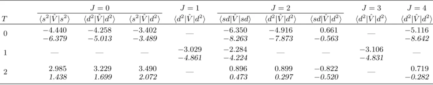
TABLE I. Two-boson interaction matrix elements hJ T|Hˆb
2|J Ti (in MeV), mapped from the KB3G interaction (IBMb, top)
and from the effective fermion interaction (IBMe, bottom).
J= 0 J= 1 J= 2 J= 3 J= 4
T hs2|Vˆ|s2i hd2|Vˆ|d2i hs2|Vˆ|d2i hd2|Vˆ|d2i hsd|Vˆ|sdi hd2|Vˆ|d2i hsd|Vˆ|d2i hd2|Vˆ|d2i hd2|Vˆ|d2i
0 −4.440
−6.379
−4.258
−5.013
−3.402
−3.489 —
−6.350
−8.263
−4.916
−7.873
0.661
−0.563 —
−5.116
−8.642
1 — — — −3.029
−4.861
−2.284
−4.224 — —
−3.106
−4.831 —
2 2.985
1.438
3.229
1.699
3.490
2.072 —
0.896
0.473
0.899
0.297
−0.822
−0.520 —
0.719
−0.282
(d), and with isospint= 1. This set corresponds to the isospin-invariant version of the IBM known as IBM-3 [35]. In the second model the set is enlarged by adding an isoscalar (p) boson with ` = 1 and t = 0 (and positive parity). The result is not the full SU(4)-invariant ver-sion of the interacting boson model known as IBM-4 [36], but it incorporates that model’s most important isoscalar correlations and therefore is situated somewhere between IBM-3 and IBM-4. We refer generically to the boson models here simply as the IBM. To refer specifically to the versions without or with the isoscalar boson, we use the terms IBM andp-IBM.
A. Mapping of the Hamiltonian
We use the order-by-order mapping described earlier to obtain the boson Hamiltonian from two- and four-nucleon systems, that is, from the A = 42 and A = 44 nuclei. The first yields the boson energies, which turn out to bes=−2.692,d =−1.322, andp=−2.350, in MeV. It also determines the structure coefficients αΓ
γ1γ2 of the collective S, D, and P pairs. In principle these may vary with mass number A to reflect the changing structure of the collective pairs. Here, however, we de-rive (boson) operators completely from the two- and four-nucleon systems. A strategy to account for the variation of the boson Hamiltonian withAis discussed below. Ac-tually, in the two-nucleon calculation there is no need to introduce effective two-body operators since the eigenval-ues and eigenvectors in the restricted Hilbert space HP
do not differ from those in the complete Hilbert spaceH. We thus derive the two-body interaction matrix ele-ments between the bosons from an analysis of the four-nucleon system. The first step here is to diagonalize the shell-model Hamiltonian in a complete two-pair basisH, following the procedure outlined in Sec. II to overcome the non-orthogonality of this basis. The resulting eigen-spectrum should coincide with the one obtained with any standard shell-model code, allowing a rigorous check of the formalism and its implementation. Next, we diag-onalize the Hamiltonian in the restricted Hilbert space
HP, which is the collective subspace defined in terms of
the pairs derived from the two-nucleon system. We will
report two different types of result: (i) one with the origi-nal “bare” shell-model Hamiltonian, and (ii) one with an effective Hamiltonian, defined by the procedure outlined in Sec. IV. The third and final step is to use the mapping procedure of Sec. V to determine the two-body part of the boson Hamiltonian. IfS and D pairs are mapped onto
sand dbosons, without considering an isoscalar P pair, then we call the resulting boson model IBMb or IBMe, depending on whether the bare or the effective shell-model Hamiltonian is used. Likewise, ifS,D, andPpairs are mapped ontos, d, andpbosons, the resulting mod-els are referred to asp-IBMb orp-IBMe. We emphasize that, unlike in the two-nucleon system, for four nucleons a realistic shell-model Hamiltonian in general couples the collective subspace to the rest of the space with poten-tially important renormalization effects. Therefore, the mapped two-body matrix elements in IBMb and IBMe may differ significantly.
The two-body matrix elements between the s and d
bosons appear in Table I, both for the “bare” KB3G interaction (IBMb) and for its effective version renor-malized to the collective subspace (IBMe). Because the largest components of theSandDpairs are in the 1f7/2 shell, we can compare the IBMe Hamiltonian with that obtained by Thompson et al. [37] from a 1f7/2 shell-model interaction. The bottom row of Table I indeed shows that the IBMe Hamiltonian resembles the one of Ref. [37]. There are some differences, notably in the
J = 0, T = 2 matrix elements, which suffer from a spu-riousd2 state in the 1f
7/2 mapping (a problem that is absent from thepfmapping), and smaller differences ap-pear because the shell-model interactions and mapping procedures (OAIversus democratic) are not exactly the same. But overall, the agreement is good.
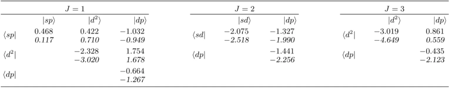
The two-body matrix elements between the s, d, and
pbosons, both for the p-IBMb and p-IBMe, are shown in Table II forT = 0 and in Table III forT = 1. TheP
pair does not influence theT = 2 matrix elements, which therefore can be taken from Table I. A general feature of the results, either with s and d, or with s, d, and p
TABLE II. Two-boson interaction matrix elements hJ T = 0|Hˆb
2|J T = 0i (in MeV), mapped from the KB3G interaction
(p-IBMb, top) and from the effective fermion interaction (p-IBMe, bottom).
J= 0 J= 2 J= 4
|s2i |d2i |p2i |sdi |d2i |p2i |d2i hs2| −3.718
−3.909
−2.476
−2.093
3.792
4.418 hsd|
−6.078
−7.978
0.477
−0.601
−1.721
−1.195 hd
2| −5.116 −8.642
hd2| −3.436 −4.147
2.187
1.984 hd
2| −4.802
−7.898
0.826
−0.065
hp2| −0.620
−1.975 hp
2| −0.327
−2.088
TABLE III. Two-boson interaction matrix elements hJ T = 1|Hˆb
2|J T = 1i (in MeV), mapped from the KB3G interaction
(p-IBMb, top) and from the effective fermion interaction (p-IBMe, bottom).
J= 1 J= 2 J= 3
|spi |d2i |dpi |sdi |dpi |d2i |dpi hsp| 0.468
0.117
0.422
0.710
−1.032
−0.949 hsd|
−2.075
−2.518
−1.327
−1.990 hd
2| −3.019 −4.649
0.861
0.559
hd2| −2.328 −3.020
1.754
1.678 hdp|
−1.441
−2.256 hdp|
−0.435
−2.123
hdp| −0.664 −1.267
takes account of correlations from outside the collective subspace.
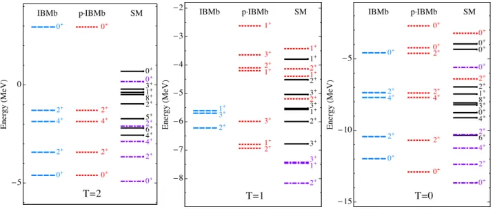
Figure 1 shows four-nucleon spectra forT = 2,T = 1, andT = 0, corresponding to low-lying levels in the nuclei 44Ca, 44Sc, and44Ti. In each case the figure shows the levels calculated in the shell model (SM) with the KB3G interaction. Some of these levels are exactly reproduced with an effective Hamiltonian constructed for a particular subspace: SM levels in dashed blue pertain to the SD
subspace and those in dotted red to theSDP subspace, while SM levels in dash-dotted purple are calculated in both subspaces. For comparison, the figure also shows the results produced by the bare KB3G Hamiltonian in the two collective subspaces.
All levels in Fig. 1 result from fermioniccalculations, in which the Pauli principle is fully taken into account, though possibly in a truncated Hilbert space. The var-ious fermionic systems are mapped onto corresponding bosonic systems, consisting of either s andd bosons, or
s,d, andpbosons. For a four-nucleon system and a bo-son Hamiltonian containing up to two-body interactions between the bosons, the mapping is exact. Therefore, the levels in the left (middle) columns of Fig. 1 are also obtained in the boson calculation with the bare Hamil-tonian of the IBMb (p-IBMb) while the colored levels in the right column are obtained in IBMe (p-IBMe).
In summary, the two-boson calculations (with the IBMe or p-IBMe Hamiltonians)exactlyreproduce the en-ergy of some eigenstates of the four-nucleon shell-model calculation. As explained in Sec. IV, the normal proce-dure is to select those that have maximal overlap with
the eigenstates in the two-pair basis. This set usually includes the yrast state but not necessarily the yrare state. For example, the shell model gives aJ = 0, T = 0 ground state at−13.668 MeV, which we also include in the (p)-IBMe; the next J = 0, T = 0 state in the two-boson calculation is at−5.601 MeV and corresponds to thethirdshell-model state with those quantum numbers. For theJ = 4 states, both withT = 0 andT = 2, we find that theD2 pair state is fragmented over the yrast and yrare shell-model states. We choose to assign the boson state to the lowest one, irrespective of the overlap; this choice conforms to the one of Thompsonet al.[37].
From Fig. 1 it is apparent that the dash-dotted pur-ple SM levels are concentrated in the low-energy region, indicating that the s and d bosons capture the essen-tial collective degrees of freedom. The same statement cannot be made about the dotted red levels, which also occur at higher energies. This is a first indication that the isoscalar p boson is not crucial for describing low-lying spectra, a fact that is not surprising in light of past work [38].
B. Mapping of the 0νββ-decay operator
ap-FIG. 1. Four-nucleon spectra forT = 2, T = 1, andT = 0, corresponding to low-lying levels in the nuclei44Ca,44Sc, and
44
Ti. The left column (dashed blue) shows all levels obtained with the bare Hamiltonian in the collective subspace constructed from S and D pairs. The middle column (dotted red) shows the same for S, D, andP pairs. The right column shows the low-energy levels obtained in the shell model with the KB3G interaction; the ones that are exactly reproduced with an effective Hamiltonian in theSDandSDP subspaces are drawn in dash-dotted purple and those that are reproduced only in theSDP
subspace in dotted red.
plied to A = 42, leads to hskTˆb
1,ββksi = −11.395 and hdkTˆ1b,ββkdi =−15.179. No 0νββ transition occurs be-tween P pairs withT = 0, and hence hpkTˆ1b,ββkpi = 0. The two-body part of the 0νββ operator is specified by the reduced matrix elementshb1b2;J TfkTˆ2b,ββkb01b02;J Tii. For the Ti = 2 → Tf = 0, Ti = 1 → Tf = 1, and
Ti = 2→Tf = 0 transitions thepboson can contribute while theTi= 2→Tf= 2 transitions are independent of thepboson.
The total 0νββ operator, both in the IBMb and
p-IBMb, and their effective versions, the IBMe and
p-IBMe, is completely specified by the reduced matrix elements hb1b2;J TfkTˆ2b,ββkb01b02;J Tii. Of course, similar mappings can be executed for separate pieces of the 0νββ
operator, such as its Gamow-Teller part. The effective-operator theory of Suzuki and Lee [24] ensures that the transition matrix elements between eigenstates in the re-stricted Hilbert spaceHP coincideexactlywith those
be-tween some of the eigenstates in the complete Hilbert spaceH.
We conclude this and the previous subsection by re-emphasizing that the formalism developed in this paper allows us to derive a boson Hamiltonian and, in general, boson operators that exactly reproduce the properties of a subset of the shell-model eigenstates of all two- and four-nucleon systems.
C. Results for the energies
We now turn to systems with more nucleons and con-sider nuclei for which a shell-model calculation is feasible in the complete Hilbert space, in order to compare its re-sults with those of the IBM. Our procedure incorporates noAdependence into the IBM operators, so that we have neither the mass-dependent structure coefficients αΓ
γ1γ2 mentioned earlier nor a dependence of the IBM Hamilto-nian on the boson numbernand isospinT, which is dis-cussed in Refs. [39, 40]. Not only is it difficult to combine the two effects but in addition the (n, T)-dependence as derived in Refs. [39, 40] applies only to a seniority-based mapping, the generalization of which to an arbitrary sys-tem of bosons is not obvious. For the purpose of this pa-per, therefore, we propose the following heuristic method to obtain anA-dependent IBM Hamiltonian and, in gen-eral,A-dependent IBM operators.
As explained in Subsec. VI A, for a given bosonic sys-tem (e.g., sd or sdp) the mapping defines a bare bo-son Hamiltonian ˆHb
b—obtained from the bare fermion Hamiltonian—as well as an effective one ˆHb
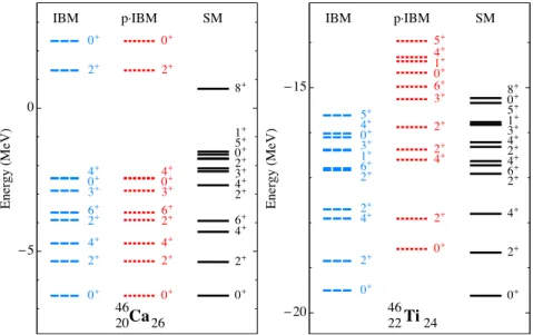
FIG. 2. Spectra of theA= 46 nuclei46Ca (T= 3) and46Ti (T= 1). The shell-model spectra (SM) are produced by the KB3G interaction with six nucleons in thepfshell. The IBM spectra, with three bosons (sdorsdp), are produced by a Hamiltonian interpolated between the bare ˆHb
b and the effective ˆHeb(see text).
following inequalities:
hHˆebin,J,T ≤ hHˆ
fi
2n,J,T ≤ hHˆ
b
bin,J,T , (52)
wherehHˆfi2n,J,T is the lowest eigenvalue, for a given nu-cleon number 2n, angular momentum J, and isospin T, of the shell-model Hamiltonian in the complete Hilbert spaceH. These inequalities suggest the use of an (n, T )-dependent boson Hamiltonian of the form
ˆ
Hb=xHˆbb+ (1−x) ˆHeb, (53)
with xan (n, T)-dependent parameter between 0 and 1 that we consider adjustable, to be determined by a com-parison with the spectrum of the shell-model Hamilto-nian in the complete Hilbert space H. By construction
x= 0 forn= 2 bosons and we expectxto increase with increasingnandT.
Figure 2 shows spectra of nuclei with mass number
A= 46; the results of the interpolation procedure can be called satisfactory. The panels in the figure are labeled with the nuclei and spectra refer to their low-energy lev-els with isospin T = |Tz|. Since isospin symmetry is conserved in both the shell model and the IBM, the cal-culated spectra in 46Ca and 46Ti are identical to those of the mirror nuclei 46Fe and 46Cr. (Because both the shell model and the IBM produce absolute energies, one would need different Coulomb corrections in the mirror nuclei.) The levels in 46Ca have isospinT = 3 and are not affected by the p bosons; the 46Ca spectra in IBM and p-IBM are consequently identical. For the T = 1 levels of 46Ti, on the other hand, the IBM and p-IBM yield different results. In the IBM a value of x can be chosen such that the binding energiesandthe excitation spectra are reasonably well reproduced. That is not the
case in thep-IBM: Ifxis adjusted to reproduce the shell-model binding energy of 46Ti, then an unrealistic exci-tation spectrum results, with a 0+-2+ energy splitting that is far too low. This difficulty confirms our suspicion that the isoscalar p boson does not play a vital role in the spectroscopy of lightpf-shell nuclei. Not only does it render the mapping to the bosonic system more complex but it also worsens the results of the simpler IBM. We have, however, yet to examine its role in 0νββ decay.
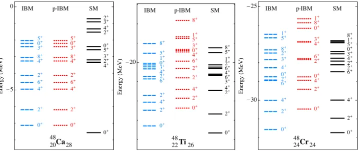
Figure 3 shows spectra for nuclei with mass number
A= 48. The boson approximation clearly breaks down in48Ca, a fact that is unsurprising because the sub-shell closure at neutron numberN−28 should cause the struc-ture of the collective pairs to change dramatically from we constructed in A = 42 nuclei. The binding energy of the 48Ca ground state is not badly wrong, however, and that particular state, which consists mostly of eight neutrons in thef7/2 shell but also includes correlations from thep3/2,f5/2, andp1/2, may still be described well enough to use in calculating the 0νββ matrix element. The spectra forA= 48, however, again confirm our state-mentpbosons do not improve spectra.
Finally, Fig. 4 shows spectra for nuclei with mass num-ber A = 50. The neutron sub-shell closure at N = 28 causes problems again in 50Ti. Unlike 48Ca, for which onlyT = 2 matrix elements enter the boson calculation, 50Ti has ground-state structure that depends onall bo-son matrix elements, including those with T = 1 and
ener-FIG. 3. Spectra of the A = 48 nuclei48Ca (T = 4), 48Ti (T = 2), and48Cr (T = 0). The shell-model spectra (SM) are produced by the KB3G interaction with eight nucleons in thepf shell. The IBM spectra, with four bosons (sdorsdp), are produced by a Hamiltonian interpolated between the bare ˆHb
b and the effective ˆHeb(see text).
FIG. 4. Spectra of theA= 50 nuclei50Ti (T = 3) and50Cr (T = 1). The shell-model spectra (SM) are produced by the KB3G interaction with ten nucleons in thepf shell. The IBM spectra, with five bosons (sdorsdp), are produced by a Hamiltonian interpolated between the bare ˆHb
b and the effective ˆHeb(see text).
gies.
D. Results for0νββ-decay transitions
We turn finally to 0νββ matrix elements. Our main interest at this point is a comparison of the results of the shell model, as reported by Men´endez et al. [19], with those of the IBM and p-IBM. The matrix elements de-pend on the values of the Hamiltonian-interpolation pa-rameterxin the initial and final nuclei. We can also
as-sign a similar parameterxββ to the 0νββoperator, that
is we can use a linear combination of the bare and effec-tive 0νββ operators the same way we do for the Hamil-tonian in Eq. (53). Here we make the simplest choice for
xββ, setting it equal to the average of the Hamiltonianx
parameters in the initial and final nuclei.
FIG. 5. Eight 0νββ0+1 →0 +
1 matrix elements betweenf7/2
-shell nuclei, calculated in the -shell model [19] and in IBM (top) andp-IBM (bottom). The full black lines connect the shell-model results and the dashed blue (dotted red) lines the IBM (p-IBM) results with anxparameter fit to energy spec-tra (see text). The shaded areas indicate upper and lower limits defined byx= 1 (bare operators) andx= 0 (effective operators).
here and in what follows. The shaded area in the figure indicates the values of the 0νββmatrix elements obtained by varying the Hamiltonian and 0νββoperators together between their bare and effective limits. This area is very large in the IBM and significantly reduced if effects of the p boson are included. Figure 6 shows the results for the Gamow-Teller part of the 0νββ matrix elements,
MGT
0ν . Thep-IBM is clearly superior to IBM in matching
the shell-model trends, although it systematically over-estimates the 0νββ matrix elements. One conspicuous feature of the shell-model calculation is the enhancement of transitions between mirror nuclei (i.e., 42Ca → 42Ti, 46Ti → 46Cr, and 50Cr → 50Fe). This p-IBM repro-duces the resulting “kink” in the calculated set of matrix Gamow-Teller matrix elements, but the IBM does not.
Despite the better performance of thep-IBM, the range of possibilities it predicts—reflected by the shaded areas that represent the plausible amount of phenomenological modification to the mapped effective operators—is large
FIG. 6. Same as Fig. 5 for the Gamow-Teller part of eight 0νββ 0+
1 →0 +
1 matrix elements betweenf7/2-shell nuclei.
enough that one could question whether apboson is re-ally essential in IBM calculations of matrix elements for the more complicated nuclei that are used in experiments. To provide a better measure of thep-boson’s importance, we examine the degree to which the IBM captures the effects of isoscalar pairing (shown repeatedly to be im-portant forββdecay [16, 19]) with and without the new degree of freedom. There is not a unique prescription for isolating the isoscalar-pairing part of the KB3G interac-tion, so we substitute the multi-separable collective in-teraction employed in Ref. [19]. This “collective” Hamil-tonian supplements the KB3G monopole part with sepa-rable like-particle pairing, isoscalar-pairing, quadrupole-quadrupole , and spin-isospin interactions, with coef-ficients determined through the methods presented in Ref. [34]. With this Hamiltonian, it is a simple matter to turn the isoscalar pairing on or off for tests.
To carry out such tests, we repeat the entire mapping procedure with the new Hamiltonian, with and without isoscalar pairing. Figure 7 shows the results for the ma-trix elements ofMGT
0ν . The left column contrasts these
FIG. 7. Same as Fig. 5 for the collective Hamiltonian without (top) and with (bottom) isoscalar pairing, and with IBM and
p-IBM results appearing in the left and right panels, respectively.
shaded band, though not small, is not unreasonable. When isoscalar pairing is turned on, shell-model matrix elements shrink considerably, except for the mirror tran-sitions. Though the IBM matrix elements also shrink on
−2
−1 0 1 2 3
s†s d†d s†s†ss s†s†dd d†d†ss d†d†dd p†p†ss p†p†dd
44Ca
→
44TiM
G
T
0
ν
IBM p-IBM
FIG. 8. Contributions to the Gamow-Teller matrix element
M0GTν from different terms in the boson Hamiltonian (see text) for the IBM (cross-hatched) andp-IBM (solid).
average, the range of predictions is much larger.
The results of thep-IBM in the right column are differ-ent, not so much in the top figure, where, as expected, the
pboson makes little difference in the absence of isoscalar pairing, but in the bottom. When the T = 0 pairing interaction is on, thep-IBM with the best value ofx re-produces the shell model results nearly perfectly, and the range of predictions is much smaller than when the pair-ing is off or when the pboson is absent. Clearly, the p
boson is required to fully capture the effects of isoscalar pairing. Even with it, however, the range of predictions grows noticeably after the boson number reaches about four.
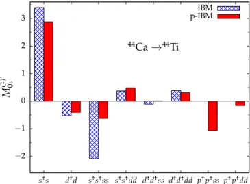
transi-tions between dbosons, is negative and relatively small. Here, however, other terms that are absent or suppressed in Ref. [11] contribute significantly. When thepboson is included, the largest contribution, outside of that from
s†s, is from p†p†ss. This operator, roughly speaking, re-places one neutron with a proton in each of twoJ = 0 neutron pairs, while recoupling the resulting pairs to an-gular momentumJ = 1 and isospinT = 0. The isoscalar-pairing interaction ensures that both the initial and final configurations are well represented in the corresponding ground states. In the absence of apboson, the IBM at-tempts to mock up the isoscalar pairs in the final nucleus by isovector proton-neutron sbosons, through the term
s†s†ss. Not surprisingly, the physics of isoscalar pair-ing is not as well captured. In the IBM-2, which does not contain neutron-proton bosons of any kind, d†d is the only term compensatings†s. One suspects that the effects of isoscalar pairing are overlooked.
VII. CONCLUSIONS
Our results clearly suggest that although the isoscalar-pair bosons have a deleterious effect on spectra—the in-evitable result of diluting collectivity—they are impor-tant for ββ decay. In our calculations with the realistic KB3G interaction, the improvement they offer is only modest, but the reason, undoubtedly, is that our map-ping is exact only for two and four nucleons and we do not know how best to extrapolate it to larger numbers. This problem plagues almost all applications of the Lee Suzuki mapping procedure.
What are the implications for the realistic IBM-2 cal-culations of Refs. [11–13, 41]? Would they be improved by the addition of apboson? Isoscalar paring is probably more effective in lightpf-shell nuclei discussed here than, e.g., in 76Ge, so we have to be a little careful in extrap-olating blindly. But many studies have shown isoscalar pairing to play a role in all the nuclei used in experiments, and thepboson thus has the potential to improve the fi-delity with which they are treated.
A useful extension of the IBM-2, however, would re-quire some careful phenomenology. The 0νββ operator in the realistic calculations, like that here, comes from a mapping of states with a few valence nucleons, and so should have similar properties to ours. But the IBM-2 Hamiltonian is entirely phenomenological and without a guiding principle and careful fitting, it is not obvious how best to modify it. One might try to map the Hamilto-nian and select from the result the most important terms that containp-boson operators, and then modify the co-efficients by fitting, e.g., to single-β decay rates (which require their own mapped operator) or other observables. Until an attempt is made, we cannot know how successful such a program would be. Our results, however, imply that it would be worthwhile.
ACKNOWLEDGMENTS
This work was partially supported (JE) by FUSTIPEN (French-U.S. Theory Institute for Physics with Exotic Nuclei) under DOE grant No. DE-FG02-10ER41700. JE also acknowledges support form the US Department of Energy under Grant Nos. FG02-97ER41019, DE-SC0008641, and DE-SC0004142. KN acknowledges sup-port from JSPS and from the Marie Curie Actions grant within the Seventh Framework Program of the European Commission under Grant No. PIEF-GA-2012-327398.
Appendix A: Matrix elements in a two-pair basis
We summarize in this appendix the expressions for the matrix element of a generic one- or two-body operator between two-pair states. Forn= 2 we rewrite the pair state (2) in a more explicitly as
|γaγbγcγd[Γ1Γ2]ΛMΛi ≡ |abcd[Γ1Γ2]ΛMΛi (A1)
∝ A X
M1M2
(Γ1M1Γ2M2|ΛMΛ)|ab; Γ1M1i |cd; Γ2M2i,
where the pair states on the last line are normal-ized and anti-symmetric, and A is a four-nucleon anti-symmetrization operator. Coupling to definite angular momentum and isospin together with anti-symmetrization leads to an expansion in terms of coeffi-cients of fractional parentage (CFPs),
|abcd[Γ1Γ2]ΛMΛi
=X
qrst
X
¯ Γ0
1¯Γ02
[qr(¯Γ01)st(¯Γ02)Λ|}abcd[Γ1Γ2]Λ]
× |qr(¯Γ01)st(¯Γ02); ΛMΛi, (A2)
where the sum{qrst}is over all permutations of{abcd}. Consider now an operator ˆTm(λλ), whereλ refers to the operator’s tensor character in angular momentum and isospin, andmλ to the respective projections. By virtue of the Wigner-Eckart theorem [42], the matrix elements of ˆTm(λλ) can be written as
ha0b0c0d0[Γ01Γ02]Λ0MΛ0|Tˆm(λ)
λ|a
00b00c00d00[Γ00
1Γ002]Λ00MΛ00i = (−)Λ0−MΛ0
Λ0 λ Λ00
−MΛ0 mλ MΛ00
× ha0b0c0d0[Γ01Γ02]Λ0kTˆ(λ)ka00b00c00d00[Γ001Γ002]Λ00i. (A3)
be expressed as
ha0b0c0d0[Γ01Γ02]Λ0kTˆ(λ)ka00b00c00d00[Γ001Γ002]Λ00i
=p X
q0r0s0t0
X
¯ Γ0
1¯Γ02
[q0r0(¯Γ01)s0t0(¯Γ02)Λ0|}a0b0c0d0[Γ01Γ02]Λ0]
× X
q00r00s00t00
X
¯ Γ00
2
[q00r00(¯Γ01)s00t00(¯Γ002)Λ00|}a00b00c00d00[Γ001Γ002]Λ00]
× hq0r0; ¯Γ01|q00r00; ¯Γ01i hs0t0; ¯Γ02kTˆ(λ)ks00t00; ¯Γ00 2i
×(−)Γ¯01+¯Γ002+Λ0+λ[Λ0][Λ00]
nΓ¯0
2 Λ0 Γ¯01 Λ00 Γ¯002 λ
o
, (A4)
with [x]≡√2x+ 1,p= 2 for a one-body andp= 6 for a two-body operator, and
hq0r0; ¯Γ01|q00r00; ¯Γ01i (A5)
= 1
1 +δq0r0
δq0q00δr0r00−(−)γq0+γr0−Γ¯
0
1δq0r00δq0r00
.
The symbol in curly brackets in Eq. (A4) refers to a prod-uct of Racah coefficients [42] in angular momentum and isospin space,
nΓ0
2 Λ0 Γ01 Λ00 Γ002 λ
o
≡n J
0
2 J0 J10
J00 J200 λj
on T0
2 T0 T10
T00 T200 λt
o
. (A6)
An important case occurs if (λ) = (0,0), that is, the tensor operator is scalar in angular momentum as well as isospin. Then Λ0 = Λ00≡Λ and the expression (A4) for the matrix element reduces to
ha0b0c0d0[Γ10Γ02]Λ|Tˆ0(0)|a00b00c00d00[Γ001Γ002]Λi
=p X
q0r0s0t0
X
¯ Γ0
1¯Γ02
[q0r0(¯Γ01)s0t0(¯Γ20)Λ|}a0b0c0d0[Γ01Γ02]Λ]
× X
q00r00s00t00
[q00r00(¯Γ01)s00t00(¯Γ20)Λ|}a00b00c00d00[Γ001Γ002]Λ]
× hq0r0; ¯Γ01|q00r00; ¯Γ01i hs0t0; ¯Γ02|Tˆ0(0)|s00t00; ¯Γ02i. (A7) This formula (withp= 6) applies to the matrix elements of a scalar two-body interaction, in which case the last factor in Eq. (A7) is the two-body matrix element,
hs0t0; Γ|Tˆ0(0)|s00t00; Γi=υsΓ0t0s00t00. (A8) The 0νββoperator can be assumed scalar in angular mo-mentum but not in isospin, and therefore requires the application of the more general expression in Eq. (A4).
Appendix B: Order-by-order mapping of non-scalar operators
For a non-scalar operator,it is better to define the boson image by requiring the equality of reduced ma-trix elements in angular momentum and isospin, defined
through the Wigner-Eckart theorem [42]. The one-boson term follows from
hbΓ0kTˆb(λ)kbΓ00i=h¯bΓ0kTˆb(λ)k¯bΓ00i=. hB¯Γ0kTˆf(λ)kB¯Γ00i. (B1) The fermion matrix element on the right-hand side of Eq. (B1) is given by
hB¯Γ0kTˆf(λ)kB¯Γ00i
=X γ0 1γ 0 2 X γ00 1γ 00 2 ¯
αΓγ00
1γ20α¯ Γ00
γ00
1γ002(−)
Γ0−MΓ0 Γ0 λ Γ00 −MΓ0 mλ MΓ00
−1
× hγ10γ20; Γ0MΓ0|Tˆmf(λλ)|γ001γ200; Γ00MΓ00i, (B2)
where hγ10γ20; Γ0MΓ0|Tˆmf(λλ)|γ 00
1γ200; Γ00MΓ00i are matrix ele-ments in the complete shell-model space and ¯αΓ
γ1γ2 are structure coefficients of normalized collective pairs,
¯
BÆM
Γ|Oi=
X
γ1γ2 ¯
αΓγ
1γ2|γ1γ2; ΓMΓi. (B3)
Equations (B1) and (B2) define entirely the one-body part ˆT1b(,mλ)
λ of the mapped boson operator. This object can be written in second quantization as
ˆ
T1b(,mλ)
λ =
X
Γ0Γ00
tΓ0Γ00(b†
Γ0טbΓ00)(mλ)
λ, (B4)
with
tΓ0Γ00 ≡
hB¯Γ0kTˆf(λ)kB¯Γ00i
√
2λ+ 1 , (B5)
an expression showing that in general ˆT1b(,mλ)λ is non-diagonal in the boson basis.
The two-body part of the mapped boson operator fol-lows from the obvious identity
hbΓ0
1bΓ02; Λ 0kTˆb(λ)
kbΓ00
1bΓ002; Λ 00i
=hbΓ0
1bΓ02; Λ 0kTˆb(λ)
1 + ˆT b(λ) 2 kbΓ00
1bΓ002; Λ
00i. (B6)
The matrix element on the left side is the boson image of the fermion operator and can be computed from Eq. (48). By using the operator representation in Eq. (B4), one can work out the first (one-body) term on the right side, obtaining
hbΓ0
1bΓ02; Λ 0kTˆb(λ)
1 kbΓ00
1bΓ002; Λ
00i (B7)
= [Λ0][λ][Λ00] ˆP(−)Γ01+Γ
0
2+Λ
00+λ
tΓ0
1Γ001
nΓ0
1 Λ0 Γ02 Λ00 Γ001 λ
o
δΓ0
2Γ002 ,
where the operator ˆP takes care of the different permu-tations: ˆP ≡PˆΓ0
1Γ02Λ0 ˆ
PΓ00
1Γ002Λ00 with ˆ
PΓ1Γ2Λ≡
f(Γ1,Γ2,Λ) + (−)Γ1+Γ2−Λf(Γ2,Γ1,Λ)
p
1 +δΓ1Γ2
Equation (B6) therefore entirely defines the two-body part ˆT2b(,mλλ) of the mapped boson operator.
As an example, we apply the above formulas to the 0νββ operator, which is a non-scalar tensor ˆTm(λλ) with
λ= (0,2) andmλ= (0,−2). It is of two-body character in the fermions and we calculate its image up to two-body terms in the bosons. We assume, as is the case in the applications discussed in this paper, that off-diagonal matrix elements between pair states vanish, that is, that
hB¯Γ0kTˆfββkB¯Γ00i = 0 if Γ0 6= Γ00. This relation obtains because the pairs have different angular momenta (S,
D and P) and the 0νββ operator is assumed scalar in
angular momentum. For two-particle states, 0νββ decay takes place from an initial state with T = 1, MT00 = +1 to a final state with T = 1, MT0 = −1, and the matrix element (B2) reduces to
hBJ T¯ kTˆfββkBJ T¯ i (B9)
=p5(2J+ 1)hJ T, MT0 =−1|Tˆfββ|J T, MT00= +1i.
The contribution (B7) of the one-body part of the boson operator between two-boson states also simplifies because Γ01 = Γ001 ≡ Γ1 and Γ02 = Γ002 ≡ Γ2, and can be written explicitly as
hbΓ1bΓ2; Λ 0kTˆb(λ)
1 kbΓ1bΓ2; Λ
00i= [Λ0][λ][Λ00](−)Γ1+Γ2+λh(−)Λ00t Γ1Γ1
nΓ1 Λ0 Γ2
Λ00 Γ1 λ
o
+ (−)Λ0tΓ2Γ2
nΓ2 Λ0 Γ1
Λ00 Γ2 λ
oi
.
(B10)
[1] R. Henning, Rev. Phys.1, 29 (2016).
[2] S. Dell’Oro, S. Marcocci, M. Viel, and F. Vissani, Adv. High Energy Phys.2016, 2162659 (2016).
[3] O. Cremonesi and M. Pavan, Adv. High Energy Phys. 2014, 951432 (2014).
[4] J. J. G´omez-Cadenas, J. Mart´ın-Albo, M. Mezzetto, F. Monrabal, and M. Sorel, Riv. Nuovo Cim. 35, 29 (2012).
[5] J. Schechter and J. W. F. Valle, Phys. Rev. D25, 2951 (1982).
[6] S. M. Bilenky and S. T. Petcov, Rev. Mod. Phys.59, 671 (1987).
[7] F. T. Avignone III, S. R. Elliott, and J. Engel, Rev. Mod. Phys.80, 481 (2008).
[8] F. F. Deppisch and J. Suhonen, Phys. Rev. C94, 055501 (2016).
[9] J. Engel and J. Men´endez, Rept. Prog. Phys.80, 046301 (2017), arXiv:1610.06548 [nucl-th].
[10] F. Iachello and A. Arima, The interacting boson model (Cambridge University Press, Cambridge, 1987). [11] J. Barea and F. Iachello, Phys. Rev. C79, 044301 (2009). [12] J. Barea, J. Kotila, and F. Iachello, Phys. Rev. C 87,
014315 (2013).
[13] J. Barea, J. Kotila, and F. Iachello, Phys. Rev. C 91, 034304 (2015).
[14] A. Arima, T. Ohtsuka, F. Iachello, and I. Talmi, Phys. Lett.66B, 205 (1977).
[15] F. Dellagiacoma and F. Iachello, Physics Letters B218, 399 (1989).
[16] P. Vogel and M. R. Zirnbauer, Phys. Rev. Lett.57, 3148 (1986).
[17] J. Engel, P. Vogel, and M. R. Zirnbauer, Phys. Rev. C 37, 731 (1988).
[18] N. Hinohara and J. Engel, Phys. Rev. C 90, 031301 (2014).
[19] J. Men´endez, N. Hinohara, J. Engel, G. Mart´ınez-Pinedo, and T. R. Rodr´ıguez, Phys. Rev. C93, 014305 (2016).
[20] J.-Q. Chen, Nuclear Physics A562, 218 (1993). [21] J.-Q. Chen, Nuclear Physics A626, 686 (1997). [22] Y. Zhao and A. Arima, Physics Reports545, 1 (2014),
nucleon-pair approximation to the nuclear shell model. [23] G. J. Fu, Y. Lei, Y. M. Zhao, S. Pittel, and A. Arima,
Phys. Rev. C87, 044310 (2013).
[24] K. Suzuki and S. Y. Lee, Prog. Theor. Phys. 64, 2091 (1980).
[25] P. Navr´atil, H. Geyer, and T. Kuo, Physics Letters B 315, 1 (1993).
[26] P. Van Isacker, International Journal of Modern Physics
E22, 1330028 (2013).
[27] T. Otsuka, A. Arima, and F. Iachello, Nucl. Phys. A 309, 1 (1978).
[28] L. D. Skouras, P. Van Isacker, and M. A. Nagarajan, Nuclear Physics A516, 255 (1990).
[29] P. L¨owdin, The Journal of Chemical Physics 18, 365 (1950), http://dx.doi.org/10.1063/1.1747632.
[30] B. C. Carlson and J. M. Keller, Phys. Rev. 105, 102 (1957).
[31] I. Mayer, International Journal of Quantum Chemistry 90, 63 (2002).
[32] A. Poves, J. S´anchez-Solano, E. Caurier, and F. Nowacki, Nucl. Phys. A694, 157 (2001).
[33] E. Caurier, G. Mart´ınez-Pinedo, F. Nowacki, A. Poves, and A. P. Zuker, Rev. Mod. Phys.77, 427 (2005). [34] M. Dufour and A. P. Zuker, Phys. Rev. C54, 1641 (1996). [35] J. P. Elliott and A. P. White, Phys. Lett. B 97, 169
(1980).
[36] J. P. Elliott and J. A. Evans, Phys. Lett. B 101, 216 (1981).
[37] M. J. Thompson, J. P. Elliott, and J. A. Evans, Phys. Lett.B195, 511 (1987).
[38] A. V. Afanasjev, (2012), arXiv:1205.2134 [nucl-th]. [39] J. A. Evans, G. Long, and J. P. Elliott, Nuclear Physics
A561, 201 (1993).
Nuclear Physics A593, 85 (1995).
[41] J. Barea, J. Kotila, and F. Iachello, Phys. Rev. D 92, 093001 (2015).
[42] I. Talmi,Simple Models of Complex Nuclei : The Shell
![FIG. 5. Eight 0νββ 0 + 1 → 0 + 1 matrix elements between f 7/2 - -shell nuclei, calculated in the -shell model [19] and in IBM (top) and p-IBM (bottom)](https://thumb-us.123doks.com/thumbv2/123dok_us/8274318.2191359/12.918.484.847.87.548/νββ-matrix-elements-shell-nuclei-calculated-shell-model.webp)