5633.pdf

(1)

TOOLS FOR PREDICTING MICROBIAL WATER QUALITY IN ESTUARIES USED FOR RECREATION AND SHELLFISH HARVESTING

Raul Alexander Gonzalez

A dissertation submitted to the faculty of the University of North Carolina at Chapel Hill in partial fulfillment of the requirements for the degree of Doctor of Philosophy in the

Department of Environmental Sciences and Engineering.

Chapel Hill 2013

(2)

ii

Abstract

RAUL ALEXANDER GONZALEZ: Tools for predicting microbial water quality in estuaries used for recreation and shellfish

(Under the direction of Rachel T. Noble)

To reduce public health risks and associated economic costs, legislation has been passed to ensure that surface waters meet standards necessary for human contact. These guidelines recommend that states routinely monitor water quality and notify the public when waters are unsafe for recreational contact or shellfish harvesting. Traditional, culture-based methods require 18-24 hours for incubation. This long processing time causes delays in the time between sample collection and public notification, which is typically on a time scale longer than that of fecal contamination events themselves. To reduce this time lag, recent national and international recommendations have placed an emphasis on the use of rapid molecular and predictive methods as tools to improve public protection. In this dissertation, I developed and applied newly approved rapid methods to predict fecal indicator bacteria (FIB) in an eastern North Carolina (NC) estuary. E. coli and enterococci concentrations can be predicted using multiple linear regression (MLR) models and a combination of antecedent rainfall, climate, and environmental variables. E. coli and enterococci models accurately predicted a high percentage (>87%) of management decisions based on regulatory thresholds. The combined assessment of quantitative PCR (qPCR) and MLR models showed both

(3)

iii

(4)

iv

Acknowledgements

First and foremost thanks to Rachel Noble, who has let me run with my ideas no matter how crazy they sounded and has always been in my corner fighting for me. Rachel gave me the opportunities to work on projects that excited me, made me proud, and allowed me to collaborate with scientists nationally and internationally.

Thanks also to my committee, Stephen Fegley, Dana Hunt, Michael Piehler, and Jill Stewart, for being great mentors and pushing me to question everything. My dissertation is a product of my committee members’ continuous guidance.

Thanks to everyone in the Noble lab, past and present, for their field and lab support. Specifically thanks to Denene Blackwood for the lunches, methodological support, and molecular advice. Also thanks to Kathy Conn and Mussie Habteselassie for teaching me about integrity and respect.

Thanks to Dana Gulbransen for being my first editor, biggest advocate, and partner in life. She was the model graduate student who I strove to become, always giving my advice and support.

(5)

v

(6)

List of Tables

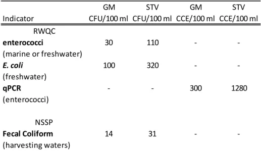
Table 1.1. Current US standards for recreational waters and shellfish harvesting waters. The 2012 recreational water quality criteria (RWQC) and 2011 National Shellfish Sanitation Program (NSSP) documents recommend both a geometric mean (GM) and STV (statistical threshold value) for monitoring water quality. The waterbody GM should not be greater than the GM shown here in any 30-day period. The NSSP does not use the term STV but in both documents the STV presented here acts as a single sample threshold in the case of one sample, and 10% of samples should not exceed this value. Values are either in colony forming units

(CFU) or calibrator cell equivalents (CCE). ...8 Table 2.1. Percent impervious cover and land use data for Ware and Oyster Creek

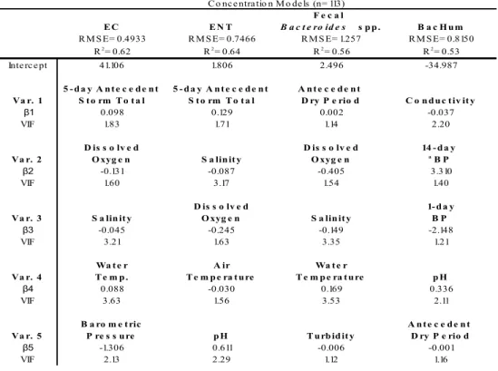
tributaries. ...38 Table 2.2. Multiple linear regression models of E. coli (EC), enterococci (ENT),

fecal Bacteroides spp., and human Bacteroides spp. (BacHum) concentrations using the training data set (n=113). Samples were collected during 12 dry and 13 wet weather events (0 – 20.3 cm of rain)

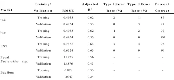
from July 2009 to August 2010. ...39 Table 2.3. Summary of E. coli (EC), enterococci (ENT), fecal Bacteroides spp.,

and human Bacteroides spp. (BacHum) model performance using the independent validation set (n=41) as compared to the training set (n=113). Error rates and percentages correct are based on predictions of

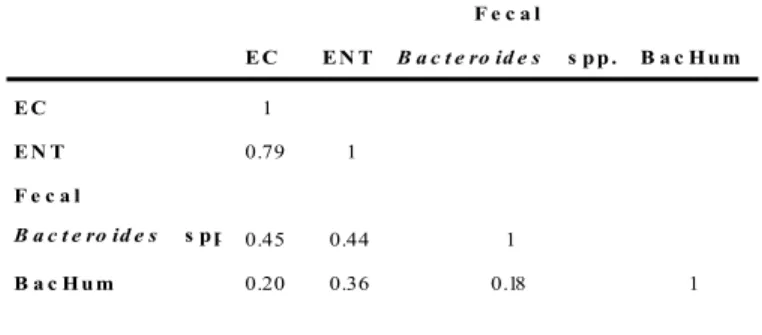
meeting or exceeding the standards for EC and ENT. ...40 Table 2.4. Pearson correlation coefficients between E. coli (EC), enterococci

(ENT), fecal Bacteroides spp., and human Bacteroides spp. (BacHum).

All corrections have a p-value <0.05...41 Table 2.5. Number of samples distributed among different strata: E. coli and

enterococci (FIB), and the Bacteroides spp. genetic markers. Number of fecal Bacteroides spp. samples shown first and number of human

Bacteroides spp. (BacHum) samples shown in parenthesis. ...42 Supplementary Table 2.1. Summary of environmental parameters collected

alongside the 151 water samples. ...43 Table 3.1. qPCR amplification efficiencies, standard curve R2 values, and

quantification range. ...71 Table 3.2. Pearson correlation coefficients between enterococci (ENT) and E.coli

(12)

xii

environmental variables. All correlations shown have p-values < 0.05

(shown in parentheses). ...72 Table 3.3. Multiple linear regression models of quantitative PCR-based

enterococci (ENT), culture-based ENT, quantitative PCR-based E. coli (EC), and culture-based EC. qPCR- and culture-based concentrations reported in CE or MPN/100 ml. Samples were collected during a wide range of meteorological and seasonal conditions from July 2009 to September 2011. Predictor variables remained untransformed during

analysis and variable regression coefficients are in parentheses. ...73 Table 3.4. Summary of quantitative PCR-based enterococci (ENT), culture-based

ENT, quantitative PCR-based E. coli (EC), and culture-based EC model performances using currently recommended, existing, or estimated FIB

thresholds. ...74 Table 3.5. Multiple linear regression model of ∆CT values to predict inhibition

levels in water samples. ...75 Table 4.1. Recreational water criteria under the BEACH Act of 2000.

Recommended indicators are E. coli (EC) and enterococci (ENT). ...102 Table 4.2. Forward and reverse primer sequences of the sketa22, fecal

Bacteroides spp, human-associated Bacteroides spp. (BacHum), and

gull2 microbial source tracking assays. ...103 Table 4.3. qPCR amplification efficiencies, R2 values, and quantification ranges

of the sketa22, fecal Bacteroides spp, human-associated Bacteroides

spp. (BacHum), and gull2 microbial source tracking assay standard

curves. ...104 Table 4.4. Fecal indicator bacteria (fecal coliforms (FC) and enterococci (ENT))

percent variation explained by the microbial source tracking markers

(fecal Bacteroides sp. and human-associated Bacteroides spp.) ...105 Table 5.1. The mean, median, variance, standard deviations, and ranges of the

fecal coliform and total Vibrio spp. time series. The monthy data sets

spanned from 5/2004 to 12/2012. ...133 Table 5.2. Periodogram analysis for the fecal coliform and total Vibrio spp. time

series using N=104 observations. ...134 Table 5.3. Multiple linear regression models using four different time lengths for

(13)

List of Figures

Figure 1.1. The Neuse River Estuary and Newport River Estuary sampling sites. Only data from site 120 of the Neuse River Estuary was used in this dissertation (chapter 5), while transects of Ware and Oyster Creeks

were used for chapters 2, 3, and 4. ...7 Figure 2.1. Ware Creek and Oyster Creek tributaries of the Newport River

Estuary in eastern North Carolina, USA. Sampling sites are denoted by black circles, weather station denoted by a black diamond, and rain

gauge by a grey diamond. ...36 Figure 2.2. Box and whisker plots of E. coli (EC), enterococci (ENT), fecal

Bacteroides spp., and human Bacteroides spp. (BacHum)

concentrations (most probable number (MPN)/100 ml or cell

equivalents (CE)/100 ml) and yields (MPN/hr/km2 or CE/hr/km2) as presented by site and weather. Box range is the 25th - 75th percentile. Whisker range is 5th-95th percentile. Means are depicted with a black square. Labeled lines indicate recreational and shellfish harvesting

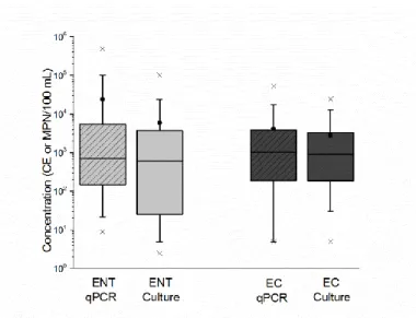
water quality thresholds. ...37 Figure 3.1. Box and whisker plots of enterococci (ENT) and E.coli (EC) (most

probable number (MPN)/100 ml or cell equivalents (CE)/100 ml) as determined by quantitative PCR and culture analytical methods. Box range is the 25th – 75th percentile. Whisker range is 5th – 95th

percentile. Means represented by solid black circles and medians are

horizontal solid lines within each box. ...70 Figure 4.1. Ware and Oyster creek tributaries of the Newport River Estuary in

eastern North Carolina. ...97 Figure 4.2. Mean fecal coliform (FC) and enterococci (ENT) concentrations

according to low and high discharge. Column error bars are + 1

standard deviation. ...98 Figure 4.3. Fecal coliform (FC) flux at Newport River Estuary headwaters by the

general rainfall categories of < 0.25 cm, > 0.25 to < 2.54 cm, and > 2.54 cm and then by the management action plan of < 3.81 cm and >

3.81 cm. Column error bars are + 1 standard deviation. ...99 Figure 4.4. Enterococci (ENT) flux at Newport River Estuary headwaters by the

general rainfall categories of < 0.25 cm, > 0.25 to < 2.54 cm, and > 2.54 cm and then by the management action plan of < 3.81 cm and >

(14)

xiv

Figure 4.5. Frequency of the fecal Bacteroides spp. and human-associated

Bacteroides spp. (BacHum) microbial source tracking markers across

low and high discharge. ...101 Figure 5.1. Ecology of infectious disease monitoring program sampling sites in

the Neuse River Estuary. Only samples from station 120 were used in our study due to the proximity to NCDENR shellfish monitoring sites

(red pentagons)...127 Figure 5.2. Graphs of fecal coliform and total Vibrio spp. time-series data. The

104 month data set spanned from May 2004 to December 2012. ...128 Figure 5.3. Lagged autocorrelation functions (ACF) for (a) fecal coliforms and (b)

total Vibiro spp. The shaded grey area is the 95% confidence interval. ...129 Figure 5.4a. The raw total Vibrio spp. time series data with the superimposed

fitted linear trend. The equation describing this trend is y = 2.5E-4x - 618. Figure 4b shows the residuals from the OLS analysis after trend

removal. ...130 Figure 5.5. The fecal coliform (FC) time series periodogram. The y-axis is

periodogram intensity (sum of squares). No significant large peaks are

apparent. ...131 Figure 5.6. The total Vibrio spp. (VIB) time series periodogram. The y-axis is

periodogram intensity (sum of squares). Two large peaks are visible at

(15)

List of Abbreviations

∆CT Comparative CT Method

ACF Autocorrelation Functions ANNs Artificial Neural Networks

ATCC American Type Culture Collection BacHum Human-associated Bacteroides spp.

BEACH Beaches Environmental Assessment and Coastal Health BMP Best Management Practice

CCE Calibrator Cell Equivalent

CE Cell Equivalent

CFU Colony Forming Unit

CT Cycle Threshold

CWA Clean Water Act

DEM Digital Elevation Model

DO Dissolved Oxygen

E. coli Escherichia coli

EC E. coli

ENT enterococci

FC Fecal coliforms

FIB Fecal Indicator Bacteria MLR Multiple Linear Regression MPN Most Probable Number MST Microbial Source Tracking

NC North Carolina

(16)

xvi

NCDMF North Carolina Department of Marine Fisheries NLCD National Land Cover Database

NOAA National Oceanic and Atmospheric Administration NPRE Newport River Estuary

NRE Neuse River Estuary

NSSP National Shellfish Sanitation Program OLS Ordinary Least Squares

PBS Phosphate Buffered Saline

qPCR Quantitative Polymerase Chain Reaction RMSE Root Mean Squared Error

RWQC Recreational Water Quality Criteria SD Standard Deviation

SPC Specimen Processing Control

SS Sum of Squares

SST Sea Surface Temperature STV Statistical Threshold Value

TCBS Thiosulfate-Citrate-Bile salts-Sucrose TMDL Total Maximum Daily Load

USEPA United States Environmental Protection Agency VIB Total Vibrio spp.

(17)

Chapter 1

INTRODUCTION

Background

Pollution of environmental waters that are used for recreation, food production, and drinking water is a major concern worldwide. Within the group of potential

contaminants, fecal pollution can account for 175 million infections annually in people who drink, bathe, or consume shellfish in polluted waters (Shuval, 2003). In addition to causing public health burdens, these fecal related infections have an added economic price in the form of health care costs and lost wages for infected individuals. One study in two California (CA) counties found that swimming related illness at 28 beaches

corresponded to an annual economic loss of $21 to $51 million in health costs alone (Given et al., 2006), while another CA study found that the health burden at only 2 beaches was $3.3 million per year (Dwight et al., 2005).

(18)

2

used for growing shellfish for human consumption to prevent illness in those that consume the shellfish produced. These guidelines recommend that states routinely monitor water quality and notify the public when waters are unsafe for contact or harvesting of shellfish.

(19)

3

marine waters. For shellfish harvesting waters, fecal coliforms, of which E. coli is the dominant subset, are used as proxies for pathogens. The use of these FIB has evolved from monitoring and successful scientific investigation linking the use of these FIB to human health outcomes. Current US standards for recreational waters and shellfish harvesting waters are in Table 1.

There are two types of FIB enumeration methods that are currently used and recommended in the new criteria document released by the EPA—traditional, culture-based methods and new, rapid molecular methods using qPCR. Traditional culture-culture-based methods, like membrane filtration and defined substrate technology tests such as IDEXX kits, require 18-24 hours for incubation. This long processing time causes a delay in the time between sample collection and public notification, which is typically on a time scale longer than that of fecal contamination events themselves (Boehm et al., 2002). During this time lag between sample collection and public notification the public can be exposed to pathogens in the water, or conversely elevated concentrations from yesterday’s sample may no longer be present in the water resulting in an unnecessary closure. Rapid methods such as qPCR can reduce processing times to 3 hours (Leecaster and Weisberg, 2001; Noble et al. 2010, Griffith and Weisberg, 2011). Strong relationships have been

demonstrated between qPCR-based FIB concentrations and human health outcomes and some studies have shown that this linkage is stronger than the relationship between culture-based FIB and health (Wade et al., 2008; Colford et al., 2012). So these molecular rapid methods are not only faster, but also more effective than traditional methods.

(20)

4

models as tools to improve public health protection. Both of these recommendations were aimed at reducing processing times and/or public notification of water closures. Well-developed predictive models can eliminate the delay between sample collection and results by providing real-time estimates of FIB concentrations at beaches. Frequently, multiple linear regression (MLR) models are used to predict recreational water quality (e.g. Olyphant et al., 2003; Olyphant and Whitman, 2004; Eleria and Vogel, 2005; Nevers and Whitman, 2005, 2011; Francy and Darner, 2007). MLR is an empirical statistical modeling approach that predicts FIB concentrations by relating water quality to antecedent rainfall, climate, and environmental parameters. When routine monitoring of beaches is not possible, MLR modeling is a useful tool for managers.

(21)

5

Although research on water quality monitoring tools is extensive for marine beaches and freshwater lakes, applications of these methods in estuarine waters,

specifically in the southeast US are limited. In estuaries, fresh water from the land mixes with saline water from the ocean, creating a dynamic environment that can provide resources for commercially important fin and shellfish (Wetz and Yoskowitz, 2013). Because of the many recreational, commercial, and ecological services provided by estuaries, it is important that managers and researchers understand the application of rapid qPCR techniques and MLR modeling in these areas.

North Carolina (NC) is one of the top beach visitation destinations in the United States, ranking 6th in beach tourism (NC Dept. of Commerce, 2013). In eastern NC there are 240 recreational monitoring sites and over 1025 shellfish harvesting water sites monitored on a regular basis. In addition, some of the locations are known as “dual beneficial use” serving both designated uses concomitantly (NCDMF, 2013). The NC Department of Environment and Natural Resources (NCDENR) conducts the monitoring programs for both recreational and shellfish harvesting waters in the state and has

expressed interest in the use of both rapid methods and predictive models to issue public health advisories in near real-time.

(22)

6

(23)

7

Figures

(24)

8

Tables

Table 1.1. Current US standards for recreational waters and shellfish harvesting waters. The 2012 recreational water quality criteria (RWQC) and 2011 National Shellfish Sanitation Program (NSSP) documents recommend both a geometric mean (GM) and STV (statistical threshold value) for monitoring water quality. The waterbody GM should not be greater than the GM shown here in any 30-day period. The NSSP does not use the term STV but in both documents the STV presented here acts as a single sample

threshold in the case of one sample, and 10% of samples should not exceed this value. Values are either in colony forming units (CFU) or calibrator cell equivalents (CCE).

GM STV GM STV

Indicator CFU/100 ml CFU/100 ml CCE/100 ml CCE/100 ml

RWQC

enterococci 30 110 -

-(marine or freshwater)

E. coli 100 320 -

-(freshwater)

qPCR - - 300 1280

(enterococci)

NSSP

Fecal Coliform 14 31 -

(25)

9

References

Boehm, A., Grant, S., Kim, J., Mowbray, S., McGee, C., Clark, C., Foley, D., Wellman, D. 2002. Decadal and shorter period variability of surf zone water quality at Huntington Beach, California. Environmental Science & Technology 36 (18), 3885-3892.

Cabelli, V. J., Dufour, A. P., McCabe, L., Levin, M. 1982. Swimming-associated gastroenteritis and water quality. American Journal of Epidemiology 115 (4), 606-616. Colford Jr, J. M., Schiff, K. C., Griffith, J. F., Yau, V., Arnold, B. F., Wright, C. C., Gruber, J. S., Wade, T. J., Burns, S., Hayes, J. 2012. Using rapid indicators for

Enterococcus to assess the risk of illness after exposure to urban runoff contaminated

marine water. Water Research 46 (7), 2176-2186.

Dwight, R. H., Fernandez, L. M., Baker, D. B., Semenza, J. C., Olson, B. H. 2005. Estimating the economic burden from illnesses associated with recreational coastal water pollution—a case study in Orange County, California. Journal of Environmental

Management 76 (2), 95-103.

Eleria, A. and Vogel, R. M. 2005. Predicting fecal coliform bacteria levels in the Charles River, Massachusetts, USA. Journal of the American Water Resources Association 41 (5), 1195-1209.

Francy, D. S. and Darner, R. A., 2007. Nowcasting beach advisories at Ohio Lake Erie beaches. Environmental Science & Technology 42 (13), 4818-4824.

Given, S., Pendleton, L. H., Boehm, A. B. 2006. Regional public health cost estimates of contaminated coastal waters: a case study of gastroenteritis at Southern California

beaches. Environmental Science & Technology 40 (16), 4851-4858.

Gonzalez, R. A., Conn, K. E., Crosswell, J. R., Noble, R. T. 2012. Application of

empirical predictive modeling using conventional and alternative fecal indicator bacteria in eastern North Carolina waters. Water Research 46 (18), 5871-5882.

Griffith, J. F. and Weisberg, S. B. 2011. Challenges in implementing new technology for beach water quality monitoring: Lessons from a California demonstration project. Marine Technology Society Journal 45 (2), 65-73.

Leecaster, M. K. and Weisberg, S. B. 2001. Effect of Sampling Frequency on Shoreline Microbiology Assessments. Marine Pollution Bulletin 42 (11), 1150-1154.

NC Department of Commerce, 2013. Fast facts, 2012 impact of visitor spending.

http://www.nccommerce.com/LinkClick.aspx?fileticket=qwtGIIJxT28%3d&tabid=636&

mid=4669.

NCDMF. 2013. North Carolina shellfish sanitation and recreational water quality section of the division of marine fisheries.

(26)

10

Nevers, M. B. and Whitman, R. L. 2011. Efficacy of monitoring and empirical predictive modeling at improving public health protection at Chicago beaches. Water research 45 (4), 1659-1668.

Nevers, M. B. and Whitman, R. L. 2005. Nowcast modeling of Escherichia coli

concentrations at multiple urban beaches of southern Lake Michigan. Water Research 39 (20), 5250-5260.

Noble, R. T., Blackwood, A. D., Griffith, J. F., McGee, C. D., Weisberg, S. B. 2010. Comparison of rapid quantitative PCR-based and conventional culture-based methods for enumeration of Enterococcus spp. and Escherichia coli in recreational waters. Applied and Environmental Microbiology 76 (22), 7437-7443.

Olyphant, G. A. and Whitman, R. L. 2004. Elements of a predictive model for

determining beach closures on a real time basis: The case of 63rd Street Beach Chicago. Environmental Monitoring and Assessment 98 (1), 175-190.

Olyphant, G. A., Thomas, J., Whitman, R. L., Harper, D. 2003. Characterization and statistical modeling of bacterial (Escherichia coli) outflows from watersheds that discharge into southern Lake Michigan. Environmental Monitoring and Assessment 81 (1), 289-300.

Prüss, A. 1998. Review of epidemiological studies on health effects from exposure to recreational water. International Journal of Epidemiology 27 (1), 1-9.

Shuval, H. 2003. Estimating the global burden of thalassogenic diseases: human

infectious diseases caused by wastewater pollution of the marine environment. Journal of Water and Health 1(2), 53-64.

Wade, T. J., Calderon, R. L., Brenner, K. P., Sams, E., Beach, M., Haugland, R., Wymer, L., Dufour, A. P. 2008. High sensitivity of children to swimming-associated

gastrointestinal illness: results using a rapid assay of recreational water quality. Epidemiology 19 (3), 375-383.

Wade, T. J., Pai, N., Eisenberg, J. N., Colford Jr, J. M. 2003. Do US Environmental Protection Agency water quality guidelines for recreational waters prevent

gastrointestinal illness? A systematic review and meta-analysis. Environmental Health Perspectives 111 (8), 1102-1109.

Wetz, M. S. and Yoskowitz, D. W. 2013. An ‘extreme’future for estuaries? Effects of extreme climatic events on estuarine water quality and ecology. Marine pollution bulletin 69 (1-2), 7-18.

(27)

Chapter 2

APPLICATION OF EMPIRICAL PREDICTIVE MODELING USING CONVENTIONAL AND ALTERNATIVE FECAL INDICATOR BACTERIA IN

EASTERN NORTH CAROLINA WATERS1

Overview

Coastal and estuarine waters are the site of intense anthropogenic influence with concomitant use for recreation and seafood harvesting. Therefore, coastal and estuarine water quality has a direct impact on human health. In eastern North Carolina (NC) there are over 240 recreational and 1025 shellfish harvesting water quality monitoring sites that are regularly assessed. Because of the large number of sites, sampling frequency often is only on a weekly basis. This frequency, along with an 18-24 hour incubation time for fecal indicator bacteria (FIB) enumeration via culture-based methods, reduces the efficiency of the public notification process. In states like NC where beach monitoring resources are limited, but historical data are plentiful, predictive models may offer an improvement for monitoring and notification by providing real-time FIB estimates. In this study, water samples were collected during 12 dry (n = 88) and 13 wet (n = 66) weather events at up to 10 sites. Predictive models for E. coli, enterococci, and members

1_{This work has been published in:}

(28)

13

of the Bacteroidales group were created and subsequently validated. Our results showed that models for E. coli and enterococci (adjusted R2 were 0.61 and 0.64, respectively) incorporated a range of antecedent rainfall, climate, and environmental variables. The most important variables for EC and ENT models were 5-day antecedent rainfall, dissolved oxygen, and salinity. These models successfully predicted FIB levels over a wide range of conditions with a 3% (EC model) and 9% (ENT model) overall error rate for recreational threshold values and a 0% (EC model) overall error rate for shellfish threshold values. Though modeling of members of the Bacteroidales group had less predictive ability (adjusted R2 were 0.56 and 0.53 for fecal Bacteroides spp. and human

Bacteroides spp., respectively), the modeling approach and testing provided information

on Bacteroidales ecology. This is the first example of a set of successful predictive

models appropriate for assessment of both recreational and shellfish harvesting water quality in estuarine waters.

2.1. Introduction

(29)

14

additional water quality management tools that do not require extensive expenditures in the form of personnel time for sample collection, processing, data analysis, and reporting.

Simple empirical predictor models can be used to maximize monitoring efficiency by providing real-time estimates of FIB concentrations. Predictor models can be used to supplement regular monitoring by identifying areas that need health warnings or more frequent monitoring, and are useful between sampling periods (USEPA, 2010).

Furthermore, in the new draft ambient water quality criteria (USEPA, 2012), USEPA strongly recommends the use of predictive models as appropriate tools to boost the effectiveness of water quality monitoring programs. In states where beach monitoring resources are limited, but historical data are plentiful, these predictive models may offer a vital improvement for monitoring and notification.

(30)

15

In eastern NC, coastal and estuarine waters are intensively used for both recreation and shellfish harvesting, with many locations simultaneously listed for both regulated uses. The NC Shellfish Sanitation and Recreational Water Quality Sections collectively monitor over 240 recreational and 1025 shellfish harvesting water locations (NCDMF, 2012). Previous work by Coulliette and Noble (2008) in the Newport River Estuary (NPRE) resulted in a presumptive rainfall closure model that recommended closing shellfish harvesting waters in the estuary after 2.54 cm of rain as opposed to the more liberal, currently used management action threshold of 3.81 cm. Additionally, Coulliette et al. (2009) created spatial/temporal maps using space-time modeling approaches that predicted elevated levels of E. coli (EC) based on rainfall and distance from land. While these models have provided useful guidance in specific conditions and in specific areas to water quality managers, they are not applicable to a wide range of estuarine and coastal locations, nor were they adequately developed over a wide range of season and conditions. The models created here are intended to provide managers with real-time estimates of FIB concentrations for dual beneficial use locations.

(31)

16

Bacteroidales, including Bacteroides thetaiotaomicron) can be indicative of a more

recent fecal contamination event given that members of this family are obligate anaerobes (Kreader, 1995; Converse et al., 2009). Because they are obligate anaerobes, routine, culture-based quantification of members of the Bacteroidales group can be time consuming. However, advances in rapid molecular methods such as quantitative

polymerase chain reaction (qPCR) have resulted in the development of many assays that estimate levels of total Bacteroidales (e.g. Total Bacteroidales: Dick et al., 2004;

“Allbac”: Layton et al., 2006; “BacUni”: Kildare et al., 2007; “GenBac”: Shanks et al., 2010) and human-associated Bacteroidales (Seurinck et al., 2005; Kildare et al., 2007; Converse et al., 2009). These qPCR assays for alternative FIB can be used in a tiered approach along with culture-based conventional FIB such as EC and ENT to provide further information on the sources of fecal contamination to receiving waters (Noble et al., 2006).

(32)

17

respectively (NSSP, 2009; USEPA, 2012). Successful model development was accomplished through three phases. First, an intensive monitoring program was implemented at two estuarine locations, including collection of data on FIB and fecal

Bacteroides spp. and human Bacteroides spp. (BacHum) concentrations, flow, loading,

and a wide range of antecedent rainfall, climate, and environmental parameters during both wet and dry conditions. Second, a training data set based on the collected monitoring data was used to develop statistical predictor models. Third, using a second, independent data set the models for EC, ENT, fecal Bacteroides spp., and BacHum were subsequently assessed.

2.2. Materials and Methods

2.2.1. Site description

(33)

18

Homer et al. (2004) and DiDonato et al. (2009). Sub-watersheds were defined in ArcGIS 9.3 based on a 1/9-arc second digital elevation model (DEM) obtained from the U.S. Geological Survey (USGS) National Map Seamless Server (http://seamless.usgs.gov). Impervious cover within each sub-watershed was calculated using the 2001 USGS

National Land Cover Database (NLCD) Zone 58 Imperviousness Layer and land use data were calculated using NLCD surface imagery classified by the U.S. Department of Agriculture National Cartography & Geospatial Center (http://www.ncgc.nrcs.usda.gov/). Impervious cover was less than 2% in both watersheds (Table 1). The dominant land uses were emergent herbaceous wetlands and evergreen forest. In addition, row crop

agriculture and developed open space (i.e. residential development) also were important land uses in the Ware Creek watershed.

2.2.2. Monitoring methods

Water samples were collected from Ware and Oyster tributaries in the NPRE (Figure 1) in the last three hours of ebb tide during 12 dry weather and 13 wet weather events between July 2009 and August 2010. Wet sampling periods were defined as events with 24 hour antecedent rain totals above 1.27 cm. This rainfall total typically results in overland flow contributions of stormwater runoff to the estuary and therefore

concomitant increases in watershed flow above dry weather levels. At each of these two sites, sampling was conducted along an upstream-to-downstream transect of 4 to 6 sampling locations spanning roughly 1400 and 1800 m (Figure 1) for a total of 151 samples. Grab samples of water were collected in sterile 1L Nalgene bottles and a multi-parameter sonde (6920 V2, YSI International, Yellow Springs, OH) was used to measure

(34)

19

water temperature. Headwater discharge was calculated from water velocity

measurements (Flow Tracker Handheld ADV®, SonTek, San Diego, CA) and tributary cross-sectional area at sites Ware 1, Oyster 1a and Oyster1b. Samples were kept on ice until processing, which occurred no more than 6 hours after sample collection. Salinity (by refractometer) and pH (by ion-selective probe) were measured in the laboratory prior to processing.

(35)

20

2.2.3. Enumeration of conventional and alternative fecal indicator bacteria

Defined Substrate Technology® kits were used to measure EC and ENT in all water samples using Colilert-18® and EnterolertTM, respectively, per manufacturer guidelines (IDEXX Laboratories, Inc., Westbrook, ME). Samples were diluted at least 1:10 in deionized water. Quantification was conducted using a 97-well most probable number (MPN) Quanti-tray®/2000 along with algorithms as previously published by Hurley and Roscoe (1983).

The alternative indicators, fecal Bacteroides spp. and BacHum, were quantified using primers, probes, and qPCR assay according to the protocols in Converse et al. (2009) and Kildare et al. (2007), respectively. A specimen processing control (SPC) was used to measure the amount of inhibition and estimate DNA extraction efficiency in each sample. Ten ng of salmon testes DNA and 500 µl of AE buffer were added to each sample, calibrator, and negative control prior to DNA extraction. DNA was recovered from polycarbonate filters (previously stored at -80˚C after filtering 50-100 ml of sample) by bead-beating following the method of Converse et al. (2009). Assays were performed in a SmartCycler® II (Cepheid Inc., Sunnyvale, CA) with the following cycling

conditions: 2 minutes at 95˚C, followed by 45 cycles of 15 seconds at 94˚C and 30 (60 for BacHum) seconds at 60˚C. Quantitative assessments of qPCR inhibition were conducted through the use of salmon testes DNA following the assay protocol of Haugland et al. (2005). Level of inhibition was assessed by calculating the difference between the cycle threshold (CT) of the SPC in the unknown sample reaction and a

(36)

21

required dilution to resolve inhibition in undiluted samples. Therefore, we tested a range of dilution levels and determined that inhibition was adequately resolved at a 1:40 dilution for 149 samples and either a 1:60 or 1:100 dilution in the remaining 5 samples. Average amplification efficiencies of the standard curves for the inhibition (salmon testes DNA), fecal Bacteroides spp., and BacHum qPCR assays were 99.7% (n=7), 99.8% (n=5), and 99.8% (n=4), respectively.

2.2.4. Data and statistical analysis

All statistics were performed in SAS 9.2 (Raleigh, NC). Instantaneous loadings (calculated based on a grab sample) of all FIB were calculated by multiplying

concentrations of EC, ENT, fecal Bacteroides spp., and BacHum (in units of either MPN/ 100 ml or cell equivalents (CE)/ 100 ml) and measured discharge (m3/ s), and reported in units of MPN (or CE)/ hr. Yields were calculated by dividing instantaneous loadings by the area of the sub-watershed. Normality was checked using histograms. Concentrations and yields were log10-transformed to reduce skewness prior to any analysis. All data were

pooled (n=151) to first examine between-creek differences and then the differences between dry and wet weather, as well as their interaction, using Scheirer-Ray-Hare tests.

(37)

22

a second randomly-selected independent set (n=41). Model performance was gauged using root mean squared error (RMSE), adjusted R2, percent type I errors, percent type II errors, and percent correct (100 – percent errors). The RMSE measured the model’s prediction capability using the independent variables, with a smaller RMSE value indicating a greater predictive capability. Adjusted R2 described the proportion of the variation that the model’s independent variables described. Type I and II errors are false positives and false negatives, respectively. An example of a type I error (false positive) is when model results recommend posting or closing a recreational or shellfish harvesting area when observed measurements indicate it should remain open. The single standard sample thresholds of 235 MPN/100 ml EC and 104 MPN/100 ml ENT for recreational water quality were used to judge error types. A threshold of 14 MPN/100 mL of EC was used to judge error types for shellfish water quality standards as a proxy for FC, a procedure which has been applied in prior work (e.g. Coulliette et al. 2009). Because there are no established recommended regulatory thresholds for fecal Bacteroides spp. and BacHum, the validation set was only judged based on RMSE and adjusted R2.

To further understand relationships between the EC and ENT and the

Bacteroidales group, we conducted an analysis of the Pearson’s correlation coefficient on

the pooled data set (n=151). Significance required a p-value < 0.05 (alpha = 0.05). In addition, to try to understand if there were any linkages across specific concentration bins, the indicators were stratified based on concentration in a manner similar to Sauer et al. (2011). EC and ENT were stratified as follows: high (>10,000 MPN/100 mL),

(38)

23

Bacteroides spp. and BacHum were stratified as follows: high (>5000 CE/100 mL),

moderate (1000-5000 CE/100 mL), and low (<1000 CE/100 mL).

2.3. Results

2.3.1. Summary statistics and loading for model development

The foundation for this modeling effort was an intensive sampling program over a wide range of environmental conditions, with culture-based quantification of EC and ENT and qPCR-based quantification of two important Bacteroidales-based markers (fecal Bacteroides spp. and BacHum). The total rainfall amounts during the wet weather events ranged from 0 to 20.3 cm and covered all seasons, making the data set broadly representative of this location. Environmental parameters and meteorological data summary are presented in Supplementary Table 1.

Means, medians, and ranges for concentrations of EC, ENT, fecal Bacteroides

spp., and the BacHum marker are shown in Figure 2. Concentrations of EC and ENT often exceeded regulatory threshold limits at both tributaries even during dry weather conditions. During dry weather 55% (48/88) of samples exceeded the recreational water quality EC threshold and 52% (46/88) exceeded the ENT threshold. During wet weather 91% (60/66) of samples exceeded the recreational water quality EC threshold and 88% (58/66) exceeded the ENT threshold. The geometric mean threshold of 14 MPN/100 mL EC for shellfish water quality was exceeded 95% (84/88) of the time in dry weather and 100% (66/66) of the time in wet weather.

(39)

24

irrespective of weather. E. coli concentrations were also significantly different between wet and dry weather conditions (p<0.001) irrespective of site. No interaction between site and weather was found (p=0.308). Similar to EC, ENT concentrations were significantly different between sites and weather conditions (p<0.001 for both), but there was also a significant interaction between site and weather for ENT concentration (p=0.031). Because there is an effect of one factor on the other, each factor was analyzed separately using a Kruskal-Wallis ANOVA. Results confirmed an ENT site (p<0.001) and weather (p<0.001) difference. For fecal Bacteroides spp. concentrations there were no significant differences between site, weather, or the interaction of site and weather (p=0.155,

p=0.240, and 0.687 respectively). BacHum concentrations were significantly different between sites and weather (p=0.005 and p<0.001, respectively), and no significant interaction between site and weather were found (p=0.304). For those with observed significant differences (EC, ENT, and BacHum), concentrations were always greater at Ware Creek than Oyster Creek and during wet weather as compared to dry weather.

(40)

25

increased significantly during wet weather. For example, mean BacHum yield to the Oyster Creek tributary increased from log 4.66 MPN/hr/km2 to log 7.88 MPN/hr/km2. No interaction effect between site and weather conditions was found for the four indicators. These summary statistics show the wide range of FIB concentrations, yields, flows, rainfall, and environmental parameters that was captured by the sampling effort, indicating the dataset is representative of this location.

2.3.2. Multiple linear regression models

Four models in total were created to predict concentrations of bacteria in a high priority estuarine system ─ one each for EC, ENT, fecal Bacteroides spp., and the BacHum marker. The models were created using data from all transect locations; therefore, the models are appropriate for any location spatially along each of the two tributaries of the NPRE. All models and their respective individual variables had significant p-values. All variables had VIFs much less than 10─ all were less than 4─ indicating no severe collinearity issues. Construction of the four concentration models, shown in Table 2, was done using a data training set (n=113). For all four concentration models, a combination of antecedent rainfall, climate (barometric pressure, air

temperature), and environmental variables (DO, salinity, pH, turbidity, conductivity) were found to maximize the FIB variation explained by the model.

(41)

26

salinity, water temperature, and barometric pressure. The RMSE was 0.4933. There was an error rate of 2% type I errors and 11% type II errors, resulting in 87% accuracy for the predictions made for recreational water quality management (Table 3). For shellfish water quality, there was an error rate of 1% type I errors and 2% type II errors resulting in 97% accuracy for model predictions (Table 3). Using this EC model on the validation set with the recreational water quality threshold, EC concentrations were predicted with 53% of the variation explained and a RMSE of 0.4954. The accuracy increased to 97%, with a 0% rate of type I errors and 3% rate of type II errors. Validating the EC model using the shellfish water quality threshold resulted in 100% accuracy in management decisions. Predictability using the EC model was considered successful based on a lower RMSE and a decrease in the error rate, even though the variance of the data set explained by the model reduced.

Similar success was found using the ENT model. The ENT model created using the training set had 64% of the data variation explained by five variables (in order of importance): 5-day antecedent rain total, salinity, dissolved oxygen, air temperature, and pH. The RMSE was 0.7466. There was an error rate of 3% type I errors and 4% type II errors, resulting in 93% accuracy in management decisions (Table 3). Using this model on the separate validation set resulted in insignificant reductions in the R2 from 0.64 to 0.63 and a change and in the management decision prediction error rate from 93% to 91%. The RMSE decreased from 0.7466 to 0.6524.

(42)

27

dissolved oxygen, salinity, water temperature, and turbidity. The BacHum model had 53% of the data variation explained by five variables (in order of importance):

conductivity, 14-day barometric pressure, 1-day barometric pressure, pH, and antecedent dry period. However, the models did not perform as well using the validation data set. The RMSE of the fecal Bacteroides spp. model increased from 1.257 to 1.438 and the adjusted R2 decreased 13%. Similarly the RMSE of the BacHum model increased from 0.8150 to 1.092 and the adjusted R2 decreased 29%.

2.3.3. Relationships between the bacterial indicator groups

To more fully understand the relationships observed between the conventional (EC and ENT) and alternative (fecal Bacteroides spp. and BacHum) indicators, we used a combination of correlation analysis and FIB stratification. All FIB concentration

comparisons had significant Pearson correlations (Table 4). The two conventional FIB were strongly correlated with each other (r=0.79, p<0.01). Fecal Bacteroides spp. had a weaker correlation to both EC and ENT (r=0.45, p<0.01 and r=0.44, p<0.01

respectively), while BacHum had a weak, but significant, correlation to both EC (r=0.20, p=0.013) and ENT (r=0.36, p<0.01). The correlation between the two Bacteroides spp. assays was weak (r=0.18, p=0.027). Table 5 shows results stratified by levels of

(43)

28

2.4. Discussion

While most water quality studies using statistical predictor models have been conducted in large urban beaches designated as recreational waters, this study evaluated the success of these models in estuarine waters with dual uses as both recreational and high priority shellfish waters. Programs that include monitoring for both uses using EC or FC (shellfish harvesting waters) and ENT (recreational waters) can put further resource strain on the monitoring agency. In estuarine systems, predictor models can conserve limited monitoring funds by identifying hot spots of chronic contamination that require more frequent monitoring while at the same time assessing contamination relationships to rainfall and identifying areas in need of presumptive rainfall closures.

2.4.1. Summary statistics and loading for model development

(44)

29

near Ware Creek and the larger percent of emergent herbaceous wetlands at Oyster Creek (67.4% as compared to 22.9 % at Ware Creek). Studies have shown that bacterial

concentrations were greatly reduced in herbaceous wetlands (Karim et al., 2004; Sleytr et al., 2007). Moreover Hemond and Benoit (1988) argue that mechanistic detention of bacteria alone by wetland vegetation can remove bacteria by allowing natural die off. A reduction in water velocity will allow sediment to drop out of the water column. Bacteria capable of particle attachment, like ENT, might then persist and grow in sediment

reservoirs. This persistent reservoir population of bacteria may contribute to the elevated FIB concentrations during dry weather.

The increase in storm fecal indicator yield, even with small amounts of precipitation, over dry weather yield also agrees well with studies conducted in other watersheds in the region (Krometis et al., 2007; Stumpf et al., 2010; Converse et al., 2011). While there was a difference in indicator concentrations between the two

tributaries, there was no difference in yield between the two tributaries. The Ware Creek watershed had more impervious cover than the Oyster Creek watershed (1.48% vs. 0.15%), but both watersheds were well below the typical percent of impervious cover at which stream quality declines (10-15%, Schueler et al., 2009).

2.4.2. Multiple Linear Regressions

(45)

30

sources such as wildlife, pets, and improperly functioning septic systems (Conn et al., 2012). Interestingly, 5-day antecedent rainfall was more important in predicting EC and ENT concentrations than the storm total or 24-hour antecedent rainfall variables. This may be because 5-day antecedent rainfall incorporates the entire hydrograph accounting for the total wet weather bacterial load. A shorter time period may only account for portions of the hydrograph and may not account for hydrographic conditions of a recent antecedent storm (e.g. storms occurring in short succession). Moreover, high antecedent rainfall can increase soil saturation levels, thereby increasing overland transport (USEPA, 2010).

The importance of salinity or conductivity in all four models also supported the important role of overland stormwater runoff in tributary bacteria concentrations. This negative relationship between salinity/conductivity and indicator concentrations suggests that as the estuarine waters are impacted by freshwater inputs (stormwater and runoff), indicator bacteria concentrations increase.

Dissolved oxygen was the second-most important variable for the EC and fecal

Bacteroides spp. models, and the third-most important variable for the ENT model. In all

three models, the variable had a negative regression coefficient. Low dissolved oxygen might be indicative of a recent contamination event such as untreated wastewater that may contain elevated bacterial levels. Low dissolved oxygen levels in surface water may also be caused by oxygen consumption as bacteria decompose organic material in runoff.

(46)

31

The fecal Bacteroides spp. model had a positive relationship while the BacHum model had a negative relationship. This may be because the target host of the two assays differs. While it was designed to preferentially quantify members of the Bacteroidales group that are relevant to the human gut, the fecal Bacteroides spp. assay also detects fecal

contamination from warm blooded animals, including wildlife. A larger number of antecedent dry days may allow a greater accumulation of fecal deposition by wildlife onto the watershed before being washed away during a storm event. On the other hand, BacHum more specifically targets human contamination. The most probable pathway of human waste into these tributaries is likely failing septic systems and therefore a signal may be more likely to occur when the antecedent dry period is short, the water table is higher, and the ground is saturated.

The prediction capabilities differed between conventional (EC and ENT) and alternative (fecal Bacteroides spp. and BacHum) indicators. The EC and ENT prediction models for recreational water quality behaved similarly to the training data set when they were applied to the validation data set. For EC, there was a slight decrease in error rate and little change in goodness-of-fit metrics for recreational water quality. For ENT, there was a decrease in RMSE and a decrease in overall error rate. By creating one model (per fecal indicator bacteria) across a diverse set of environmental conditions and spatially diverse locations, conventional FIB can now accurately be predicted in real-time at our study sites for recreational water quality standards. Future work will validate these models in the whole estuary and other similar estuaries nearby.

Bacteroidales model prediction within the same estuary allowed insight into what

(47)

32

training data set, members of the Bacteroidales group were found to have strong linear relationships to many of the parameters tested (e.g. antecedent dry period, dissolved oxygen, conductivity, barometric pressure, water temperature, turbidity). Additionally the low prediction power of the qPCR-based models may be due to the elevated lower limit of method detection caused by sample inhibition. Because the estuarine samples were highly inhibited, samples for qPCR processing had to be diluted. This dilution weakened the performance of the model at lower concentrations and may be the reason for the lower amount of variation explained by the model. Future work including the use of commercial DNA extraction kits to reduce the presence of inhibitory compounds and the use of a larger validation dataset should be done to enhance Bacteroidales prediction.

2.4.3. Relationship between the bacterial groups

Results from the correlation analysis indicate a strong relationship between EC and ENT concentrations in these two tributaries of the NPRE. This suggests that EC and ENT likely originate from similar sources and have similar physical process affecting their ecology. However, there was a weak relationship between the conventional FIB (EC and ENT) and the Bacteroides spp. indicators, as indicated by low, but significant,

Pearson correlation coefficients. The low concordance of high ranking EC and ENT to high ranking Bacteroidales members (Table 5) support the idea that other contamination sources exist besides warm-blooded mammals. Specifically, only 10 out of 18 high priority samples (EC and ENT > 10,000 MPN/ 100 ml) had moderate or high fecal

Bacteroides spp. concentrations and merely 2 out of 18 high EC and ENT samples had

(48)

33

ENT are facultative anaerobes that can survive, and even grow, in aerobic environments. EC and ENT likely originate from a variety of land-based sources that are delivered to the estuary by overland runoff, especially during storm events. Both EC and ENT may also persist in the environment (i.e. bed sediment) and contribute to elevated

concentrations during dry weather, perhaps due to resuspension. Additionally, the weak relationship between Bacteroides spp. and conventional FIB may also be a byproduct of different enumeration methods. The conventional FIB were enumerated using culture based methods (measures metabolically active cells), while the Bacteroidales groups were enumerated through the amplification of target DNA. In order to rectify this problem, future work will compare EC, ENT, fecal Bacteroides spp., and the BacHum marker using only qPCR-based methods.

2.4.4. Application

(49)

34

and regionally. Using parameters measured in-situ or retrieved online such as antecedent rainfall, dissolved oxygen, and salinity, real-time EC and ENT predictive models

presented in this study can supplement monitoring and improve notifications of closures during both wet and dry weather conditions. Because of the robust sampling approach and data collection program, we anticipate that models like these could be relevant to both shellfish harvesting and recreational waters in similar regions in NC, Virginia, and other shallow, lagoon estuarine locations that are the prominent sites of much shellfish harvesting and recreation. Additionally, managers using these models can have the economic advantage of using a single model across locations while predicting a high percentage of correct management decisions.

2.5. Conclusions

 Water samples in the recreational and high priority shellfish harvesting waters of the NPRE often exceeded NC water quality thresholds, even during dry weather.

 Concentrations of the fecal indicator bacteria, ECand ENT, can be predicted using empirical statistical models and a combination of antecedent rainfall, climate, and environmental variables including 5-day antecedent rainfall, dissolved oxygen, and salinity.

 ECand ENT models accurately predicted a high percentage (>87%) of management decisions based on current regulatory thresholds.

(50)

35

(51)

36

Figures

(52)

37

Figure 2.2. Box and whisker plots of E. coli (EC), enterococci (ENT), fecal Bacteroides

(53)

38

Tables

Wa re C re e k Oys te r C re e k

P e rim e te r: 5,712 m 7,487 m

Are a : 0.14 km 2 0.31 km 2

Appro x. c re e k le ngth (inc . tributa rie s ): 1,778 m 1,407 m

La nd C o ve r % %

De ve lo pe d, Ope n S pa c e 12.1 0

Eve rgre e n F o re s t 19.3 21.3

M ixe d F o re s t 0 0.58

S hrub/S c rub 0.6 0.58

Gra s s la nd/He rba c e o us 11.5 6.71

P a s ture /Ha y 5.42 0

C ultiva te d C ro ps 21.7 0.58

Wo o dy We tla nds 6.63 2.29

Em e rge nt He rba c e o us We tla nds 22.9 67.4

% Im pe rvio us C o ve r 1.48 0.15

(54)

39

E C E N T B a c H u m

R M S E= 0.4933 R M S E= 0.7466 R M S E= 1.257 R M S E= 0.8150

R2_{= 0.62} _R2_{= 0.64} _R2_{= 0.56} _R2_{= 0.53}

Inte rc e pt 41.106 1.806 2.496 -34.987

5 - d a y A n t e c e d e n t 5 - d a y A n t e c e d e n t A n t e c e d e n t

Va r. 1 S t o rm T o t a l S t o rm T o t a l D ry P e rio d C o n d u c t iv it y

β1 0.098 0.129 0.002 -0.037

VIF 1.83 1.71 1.14 2.20

D is s o lv e d D is s o lv e d 14 - d a y Va r. 2 O xyg e n S a lin it y O xyg e n a_{B P}

β2 -0.131 -0.087 -0.405 3.310

VIF 1.60 3.17 1.54 1.40

D is s o lv e d 1- d a y Va r. 3 S a lin it y O xyg e n S a lin it y B P

β3 -0.045 -0.245 -0.149 -2.148

VIF 3.21 1.63 3.35 1.21

Wa t e r A ir Wa t e r

Va r. 4 T e m p . T e m p e ra t u re T e m p e ra t u re p H

β4 0.088 -0.030 0.169 0.336

VIF 3.63 1.56 3.53 2.11

B a ro m e t ric A n t e c e d e n t Va r. 5 P re s s u re p H T u rb id it y D ry P e rio d

β5 -1.306 0.611 -0.006 -0.001

VIF 2.13 2.29 1.12 1.16

a_{B P =B a ro m e tric P re s s ure}

C o nc e ntra tio n M o de ls (n= 113)

F e c a l

B a c t e ro id e s s p p .

Table 2.2. Multiple linear regression models of E. coli (EC), enterococci (ENT), fecal

Bacteroides spp., and human Bacteroides spp. (BacHum) concentrations using the

(55)

40

T ra in in g / A d ju s t e d T yp e I E rro r T yp e II E rro r P e rc e n t M o d e l _{Va lid a t io n} _{R M S E} R2

R a t e ( %) R a t e ( %) C o rre c t

Tra ining 0.4933 0.62 2 11 87

Va lida tio n 0.4954 0.53 0 3 97

Tra ining 0.4933 0.62 1 2 97

Va lida tio n 0.4954 0.53 0 0 100

Tra ining 0.7466 0.64 3 4 93

Va lida tio n 0.6524 0.63 0 9 91

Tra ining 1.2573 0.56 - -

-Va lida tio n 1.4376 0.43 - -

-Tra ining 0.815 0.53 - -

-Va lida tio n 1.0919 0.24 - -

-a_{EC m o de l va lida te d with re c re a tio na l wa te r qua lity thre s ho ld} b_{EC m o de l va lida te d with s he llfis h ha rve s ting wa te r qua lity thre s ho ld} a_EC

ENT

B a c Hum F e c a l

B ac te ro ide s s pp.

b_EC

(56)

41

F e c a l

E C E N T B a c t e ro id e s s p p . B a c H u m

E C 1

E N T 0.79 1

F e c a l

B a c H u m 0.20 0.36 0.18 1

0.45 0.44 1

Table 2.4. Pearson correlation coefficients between E. coli (EC), enterococci (ENT), fecal

Bacteroides spp., and human Bacteroides spp. (BacHum). All corrections have a p-value

(57)

42

N o . s a m p le s wit h h ig h F IB

N o . s a m p le s wit h m o d e ra t e F IB

N o . s a m p le s wit h lo w F IB

(>10,000 M P N/100 m l) (1000-10,000 M P N/100 m l) (<1000 M P N/100 m l)

N o . s a m p le s wit h h ig h

(>5000 C E/100 m l)

N o . s a m p le s wit h m o d e ra t e

(1000-5000 C E/100 m l)

N o . s a m p le s wit h lo w

(<1000 C E/100 m l)

6(0)

8(16)

16(1) 10(0)

26(47) 66(81)

4(2) 12(6) 6(1)

(58)

43

S a lin it y Wa t e r T u rb id it y D is s o lv e d Wa t e r 2 4 - h r R a in A ir T e m p . B a ro m e t ric ( p p t ) p H T e m p . (˚C ) ( N T U) O xyg e n ( m g / L) Ve lo c it y ( m / s ) T o t a l ( c m ) (˚C ) P re s s u re ( in H g )

N to ta l 149 149 129 137 134 120 151 151 151

M e a n 15.9 7.31 23.6 80.5 6.29 0.17 3.38 23.4 29.9

S ta nda rd De via tio n 12.6 0.65 6.52 98.1 2.54 0.27 5.16 5.09 0.19

M inim um 0 3.85 10.4 0.70 0.81 -0.11 0.00 7.22 29.4

M a xim um 35.0 8.42 36.7 628 11.4 1.31 20.3 30.6 30.2

Inte rqua rtile R a nge 25.0 0.79 10.9 77.3 3.18 0.25 4.29 8.00 0.22

90th P e rc e ntile 32.0 8.07 31.6 205 9.88 0.59 9.25 29.7 30.12

95th P e rc e ntile 35.0 8.14 33.1 277 10.6 0.73 14.6 30.6 30.18

99th P e rc e ntile 35.0 8.39 35.6 470 11.3 1.27 20.3 30.6 30.18

(59)

44

References

Bernhard, A. E. and Field, K. G., 2000. Identification of nonpoint sources of fecal pollution in coastal waters by using host-specific 16S ribosomal DNA genetic markers from fecal anaerobes. Applied and Environmental Microbiology 66(4), 1587-1594. Characklis, G. W., Dilts, M. J., Simmons III, O. D., Likirdopulos, C. A., Krometis, L. H., Sobsey, M. D., 2005. Microbial partitioning to settleable particles in stormwater. Water Research 39(9), 1773-1782.

Conn, K. E., Habteselassie, M. Y., Blackwood, A.D., Noble, R. T., 2012. Microbial water quality before and after the repair of a failing onsite wastewater treatment system

adjacent to coastal waters. Journal of Applied Microbiology 112(1), 214-224.

Converse, R. R., Piehler, M. F., Noble, R. T., 2011. Contrasts in concentrations and loads of conventional and alternative indicators of fecal contamination in coastal stormwater. Water Research 45(16), 5229-5240.

Converse, R. R., Blackwood, A. D., Kirs, M., Griffith, J. F., Noble, R. T., 2009. Rapid QPCR-based assay for fecal Bacteroides spp. as a tool for assessing fecal contamination in recreational waters. Water Research 43(19), 4828-4837.

Coulliette, A. D. and Noble, R. T., 2008. Impacts of rainfall on the water quality of the Newport River Estuary (eastern North Carolina, USA). Journal of Water and Health 06(4), 473-482.

Coulliette, A. D., Money, E. S., Serre, M. L., Noble, R. T., 2009. Space/time analysis of fecal pollution and rainfall in an eastern North Carolina estuary. Environmental Science & Technology 43(10), 3728-3735.

Dick, L. K. and Field, K. G., 2004. Rapid estimation of numbers of fecal Bacteroidetes

by use of a quantitative PCR assay for 16S rRNA genes. Applied and Environmental Microbiology 70(9), 5695-5697.

DiDonato, G. T., Stewart, J. R., Sanger, D. M., Robinson, B. J., Thompson, B. C., Holland, A. F., Van Dolah, R. F., 2009. Effects of changing land use on the microbial water quality of tidal creeks. Marine Pollution Bulletin 58(1), 97-106.

(60)

45

Francy, D. S., 2009. Use of predictive models and rapid methods to nowcast bacteria levels at coastal beaches. Aquatic Ecosystem Health and Management Society 12(2), 177-182.

Francy, D.S., Bertke, E.E., and Darner, R.A., 2009. Testing and refining the Ohio Nowcast at two Lake Erie beaches—2008: U.S. Geological Survey Open-File Report 2009–1066, 19 p.

Griffith, J. F., and Weisberg, S. B., 2011. Challenges in implementing new technology for beach water quality monitoring: Lessons from a California demonstration project. Marine Technology Society Journal 45(2), 67-73.

Hathaway, J. M., Hunt, W. F., Simmons III, O. D., 2010. Statistical evaluation of factors affecting indicator bacteria in urban storm-water runoff. Journal of Environmental Engineering 136(12), 1360-1368.

Haugland, R. A., Siefring, S. C., Wymer, L. J., Brenner, K. P., Dufour, A. P., 2005. Comparison of Enterococcus measurements in freshwater at two recreational beaches by quantitative polymerase chain reaction and membrane filter culture analysis. Water Research 39(4), 559-568.

Hemond, H. F. and Benoit, J., 1988. Cumulative impacts on water quality functions of wetlands. Environmental Management 12(5), 639-653.

Homer, C., Huang, C., Yang, L., Wylie, B., Coan, M., 2004. Development of a 2001 national landcover database for the United States. Photogrammetric Engineering & Remote Sensing 70(7), 829-840.

Hurley, M. A. and Roscoe, M. E. (1983) Automated statistical analysis of microbial enumeration by dilution series. Journal of Applied Microbiology 55(1), 159-164. Karim, M. R., Manshadi, F. D., Karpiscak, M. M., Gerba, C. P., 2004. The persistence and removal of enteric pathogens in constructed wetlands. Water Research. 38(7), 1831-1837.

Kildare, B. J., Leutenegger, C. M., McSwain, B. S., Bambic, D. G., Rajal, V. B., Wuertz, S., 2007. 16S rRNA-based assays for quantitative detection of universal, human-, cow-, and dog-specific fecal Bacteroidales: A Bayesian approach. Water Research 41(16), 3701-3715.

Kreader, C. A., 1995. Design and evaluation of Bacteroides DNA probes for the specific detection of human fecal pollution. Applied and Environmental Microbiology 61(4), 1171-1179.

5633.pdf

Abstract

Acknowledgements

Table of Contents

List of Tables

List of Figures

List of Abbreviations

Chapter 1

Chapter 2