SIMULATING EPIDEMICS AND INTERVENTIONS ON HIGH RESOLUTION SOCIAL NETWORKS
A Thesis presented to
the Faculty of California Polytechnic State University, San Luis Obispo
In Partial Fulfillment
of the Requirements for the Degree Master of Science in Computer Science
by
COMMITTEE MEMBERSHIP
TITLE: Simulating Epidemics and Interventions on High Resolution Social Networks
AUTHOR: Christopher E. Siu
DATE SUBMITTED: June 2019
COMMITTEE CHAIR: Theresa Migler-VonDollen, Ph.D.
Assistant Professor of Computer Science
COMMITTEE MEMBER: John Clements, Ph.D.
Professor of Computer Science
COMMITTEE MEMBER: Nathaniel Martinez, M.D., Ph.D.
Assistant Professor of Biological Sciences
COMMITTEE MEMBER: Julie Workman
ABSTRACT
Simulating Epidemics and Interventions on High Resolution Social Networks Christopher E. Siu
Mathematical models of disease spreading are a key factor of ensuring that we are prepared to deal with the next epidemic. They allow us to predict how an infection will spread throughout a population, thereby allowing us to make intelligent choices when attempting to contain the disease. Whether due to a lack of empirical data, a lack of computational power, a lack of biological understanding, or some combination thereof, traditional models must make sweeping assumptions about the behavior of a population during an epidemic.
ACKNOWLEDGMENTS
Thanks to:
• To my advisor, Professor Theresa Migler-VonDollen: you have given me so much support and encouragement over the last three years. You helped me discover my interest in theoretical computer science, and you constantly demonstrate the quality I strive for as an educator.
• To Professor John Clements: in many ways, your classes were my first intro-duction to navigating academia, both as a graduate student and as a novice researcher.
• To Professor Nathaniel Martinez: I am not an epidemiologist; I am not even a biologist. Your expertise and input provided invaluable guidance towards pragmatic, relevant applications for my work.
• To Professors Julie Workman and Paul Hatalsky: you taught me everything I know about the fundamentals of computer science. You helped me realize my interest and belonging in this field, and, because of you, the dream job I didn’t yet know what I wanted practically fell into my lap when I was nineteen.
• To Jon, Caleb, and Chris: I have wasted countless hours in video games and on the Internet because of you three, and I don’t regret any of it. You should have stayed in grad school with me — who needs money?
TABLE OF CONTENTS
Page
LIST OF TABLES . . . x
LIST OF FIGURES . . . xi
CHAPTER 1 Introduction . . . 1
2 Background . . . 3
2.1 Epidemiological Models . . . 3
2.2 Compartmental Models . . . 4
2.2.1 Susceptible-Infected-Recovered . . . 5
2.2.2 Susceptible-Infected-Susceptible . . . 5
2.2.3 SIRS, SEIR, MSIR, and Other Models . . . 6
2.3 Full Mixing Simulations . . . 6
2.4 Epidemiological Metrics . . . 7
2.4.1 Basic Reproduction Number . . . 8
2.4.2 Epidemic and Herd Immunity Thresholds . . . 8
2.5 Graphs . . . 9
2.6 The Copenhagen Network Study . . . 11
3 Related Works . . . 15
3.1 Disease Spreading on Graphs . . . 15
3.2 Disease Spreading with Mobility Patterns . . . 16
3.3 Disease Spreading on Graphs with Mobility Patterns . . . 18
4.1 Preprocessing . . . 21
4.2 Graph Representation . . . 22
4.3 Simulation Architecture . . . 24
4.3.1 The Flu Model . . . 24
4.3.2 The Measles Model . . . 26
4.3.3 The Norovirus Model . . . 28
4.4 Interventions . . . 31
4.4.1 Uniform Vaccination . . . 33
4.4.2 Vaccination by Degree Distribution . . . 33
4.4.3 Vaccination by k-Cores . . . 36
4.4.4 Vaccination by Density Decomposition . . . 37
4.4.5 Quarantining . . . 38
4.5 Summary of Simulations . . . 39
5 Methodology . . . 42
5.1 Baseline Models . . . 42
5.2 Models with Interventions . . . 43
6 Results . . . 46
6.1 Baseline Scenarios . . . 46
6.1.1 Influenza . . . 46
6.1.2 Measles . . . 49
6.1.3 Norovirus . . . 50
6.2 Uniform Vaccination . . . 53
6.3 Targeted Vaccination . . . 56
6.3.1 Vaccination by Degree . . . 56
6.3.3 Vaccination by Ring . . . 58
6.4 Quarantine Scenarios . . . 61
7 Conclusion . . . 64
7.1 Future Work . . . 64
7.1.1 Ineffective Vaccinations . . . 64
7.1.2 Additional Community Detection Algorithms . . . 64
7.1.3 Combinations of Interventions . . . 65
7.1.4 Simultaneous Infections . . . 65
7.1.5 External Contacts and Deaths . . . 66
7.2 Summary of Contributions . . . 66
LIST OF TABLES
Table Page
LIST OF FIGURES
Figure Page
1 Compartments of Bernoulli’s Model . . . 4
2 The SEIR Model . . . 5
3 Drawing of The Seven Bridges of Königsberg . . . 9
4 Graph of the Seven Bridges of Königsberg . . . 10
5 Cliques and Stars . . . 11
6 The SEIR Model Applied to a Social Network . . . 11
7 Selected Interactions in the Copenhagen Network Study . . . 12
8 Interactions by Time in the Copenhagen Dataset . . . 14
9 Numbers of Unique Interactions in the Copenhagen Dataset . . . . 14
10 Graph Snapshot of One Timestamp . . . 23
11 Cluster Detection over Four Snapshots . . . 29
12 Example Degree Distribution . . . 34
13 Example Flattened Graph . . . 35
14 Example k-Cores . . . 36
15 Affected Individuals in a Baseline Influenza Scenario . . . 47
16 Affected Individuals in Baseline Influenza Scenarios . . . 48
17 Infected Individuals in Baseline Influenza Scenarios . . . 48
18 Affected Individuals in Baseline Measles Scenarios . . . 50
19 Exposed and Infected Individuals in Baseline Measles Scenarios . . 51
20 SEIR Compartments in a Baseline Measles Scenario . . . 51
23 SEIR Compartments in a Uniform Vaccination Scenario . . . 54
24 Affected Individuals in Uniform Vaccination Scenarios . . . 55
25 Summary of Uniform Vaccination Scenarios . . . 55
26 Affected Individuals when Vaccinated by Degree . . . 57
27 Affected Individuals when Vaccinated by k-Core . . . 59
28 Affected Individuals when Vaccinated by Ring . . . 60
29 Affected Individuals in Quarantine Scenarios . . . 63
Chapter 1
INTRODUCTION
“Epidemich…a sicknesse common vnto all people, or to the moste part of them.” — Thomas Lodge, A Treatise of the Plague, 1603
From the Greek “επιδηµιος” via the French “épidémique”, the word “epidemic” was first used in the English language in 1603, and it has come to describe a disease which has quickly infected an unusually high number of people within some well-defined population (OED Online, n.d.). Epidemics may further be termed “pandemics” to distinguish those diseases which have spread on a continental or global scale, and epidemics may be contrasted with “epizootics”, which affect animals.
Epidemiology, then, is the study of diseases that infect people, including the bio-logical and social mechanisms involved in their outbreak, transmission, containment, and, hopefully, eventual eradication. Of that last goal, to date, only one disease that affects humans has been eradicated: a naturally occurring case of smallpox has not been reported since October of 1977, the conclusion of almost two hundred years of work immunizing the general population (Fenner, Henderson, Arita, Jezek, & Ladnyi, 1988). This required a dedicated program on the part of the World Health Organiza-tion, involving mass vaccinations, health surveilance, and targeted interventions on continental scales over more than a decade.
us to contain outbreaks before they become epidemics, and, failing that, to determine the appropriate methods of intervention. Mathematical approaches for studying dis-eases have existed for just about as long — slightly longer, in fact — as the vaccination processes that can prevent them (Dietz & Heesterbeek, 2002). However, because of the complexity of the involved social and biological mechanisms, traditional math-ematical models must make a handful of key unrealistic assumptions. They cannot account for the transmission of disease on an individual, per-person scale.
Chapter 2
BACKGROUND
2.1 Epidemiological Models
Use of mathematical models to characterize the spread of disease and explore potential treatments dates to around 1766, when Daniel Bernoulli developed a simplistic model to investigate the feasibility of inoculation against smallpox (Dietz & Heesterbeek, 2002), inoculation being the primitive precursor to vaccination. He reasoned that the population could be divided into two groups: those who had not yet contracted the disease, and were therefore susceptible, and those who had already survived the disease, and were therefore immune. In Bernoulli’s model, surviving smallpox moves an individual from the susceptible group to the immune group; death removes an individual from their current group.
Susceptible Immune s(a)λ(a)
µ(a) + [1−s(a)]λ(a) µ(a)
Figure 1: Compartments of Bernoulli’s Model. Here,ais age,λ(a)is
probabil-ity of infection,s(a)is that of survival, andµ(a)is that of death by other causes. (Di-etz & Heesterbeek, 2002)
2.2 Compartmental Models
In the modern nomenclature, Bernoulli’s work employs a simplecompartmental model: a model that divides the population into “compartments”, depending on how the dis-ease has already affected or might potentially affect them. The movement of an indi-vidual between compartments is governed by a simple, typically probabilistic, state machine. Namely, Bernoulli’s model has “Susceptible” and “Immune” compartments, reproduced in Figure 1.
2.2.1 Susceptible-Infected-Recovered
These historical models are most similar to the modern Susceptible-Infected-Recovered, or SIR, model, which has direct analogs to their compartments. In this model, every individual is either at risk of contracting the disease, currently infected and capable of transmitting the infection, or immune (whether by recovery or by death).
2.2.2 Susceptible-Infected-Susceptible
Depending on the particular disease that we are interested in modeling, the Susceptible-Immune compartments may be too simplistic, and the Susceptible-Infected-Recovered compartments, outright inaccurate. Surviving influenza, for example, does not make an individual immune to alternative strains and future mutations of the virus (Kram-mer et al., 2018). If we were interested in simulating influenza on time scales long enough for this to matter (and if we made the questionably realistic assumption that all strains could be simulated as the same disease), we might apply the Susceptible-Infected-Susceptible model (SIS), in which individuals are once again at risk after having recovered.
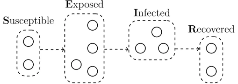
Susceptible
Exposed
Infected
Recovered
Figure 2: The SEIR Model. This example population is divided into Susceptible,
2.2.3 SIRS, SEIR, MSIR, and Other Models
There are, unsurprisingly, a plethora of variations on the basic compartmental mod-els, depending the disease and desired granularity of the particular application. The previously mentioned influenza outbreaks, whose strains can change from year to year, also tend to occur in seasonal patterns (Krammer et al., 2018), so a model that allows for a temporary period of effective immunity may be more appropriate. Malaria has a non-trivial incubation time (Phillips et al., 2017), so a model should allow for the possibility that an individual has been infected but does not yet exhibit any symptoms. Infants inherit about nine months of immunity to measles from their mother (Rota et al., 2016), so a model may need to include this initial period. Mod-els such as Susceptible-Infected-Recovered-Susceptible (SIRS), Susceptible-Exposed-Infected-Recovered (SEIR), and Maternal-Susceptible-Susceptible-Exposed-Infected-Recovered (MSIR) at-tempt to account for these situations, respectively. An example of the SEIR model is depicted in Figure 2.
2.3 Full Mixing Simulations
equal chance of coming into contact with any other member of the population, and, thus, an equal chance of contracting the disease via that contact (itself an unrealistic assumption in the case of the bubonic plague, which spreads via fleas that live on rats (McEvedy, 1988)). Kermack and McKendrick therefore conclude that “None of these conditions are strictly fulfilled and consequently the numerical equation can only be a very rough approximation.”
Nevertheless, traditional epidemic modeling continues to use the same general ap-proach. Given a sequence of compartments describing the possible states and transi-tions of infected individuals, they simulate the spread of disease by using differential equations to describe the movements of individuals between compartments. To some extent, these systems of equations can be extended to approximate the interactions of individuals (Murray, Stanley, & Brown, 1986). In effect, impersonal though it may seem, we may think of individuals in different states as a mix of different fluid chemicals in a reaction-diffusion system. In this application, the “chemical reactions” are the transmission of disease from contagious individuals to susceptible individuals, while “diffusion” describes the random movement of those individuals throughout the population.
2.4 Epidemiological Metrics
2.4.1 Basic Reproduction Number
Thebasic reproduction number R0 is the number of individuals we can expect a single contagious host to infect over the duration of their infectious period, assuming that every other individual is susceptible. In order for the disease to spread, R0 must be strictly greater than1. The specific number will vary from disease to disease, and can be estimated from empirical data from past outbreaks. A higher basic reproduction number implies a more virulent disease. Since we know how many unique contacts the average individual makes in one day in our dataset, and we know how many days such an individual remains infectious, the basic reproduction number is all we need to estimate the probability of transmission per contact.
2.4.2 Epidemic and Herd Immunity Thresholds
By definition, if an individual is immune to a disease, they will not contract the disease. Thus, generally speaking, if an individual is immune to a disease, they are incapable of spreading it. Therefore, as the fraction of the population that is immunized rises, the spreading of the disease is impeded, as there are fewer contacts by which it can be transmitted. If enough of the population is immune, an infectious individual may not have enough opportunities to spread the disease to the entire susceptible population, a phenomenon known as “herd immunity”.
The epidemic threshold βc is the fraction of individuals that must be susceptible in
order for a disease to persist. Below this threshold, the disease can be expected to die out before spreading beyond its local susceptible population. Alternatively, (1− βc) is the herd immunity threshold, the fraction of individuals that must be
Figure 3: Drawing of The Seven Bridges of Königsberg. Euler’s illustration of the Seven Bridges labels the landmasses asA,B,C, and D. (Euler, 1741)
predictions, however, assume a full mixing model, and are therefore not applicable to our simulations.
2.5 Graphs
Perhaps by coincidence, at almost the same time Daniel Bernoulli was modeling dis-eases with compartments, Leonhard Euler was considering the bridges that connected an island in the Pregel River with then-Königsberg, Prussia. To solve the problem that has become known as the Seven Bridges of Königsberg, Euler developed what he called the “geometry of position” (Euler, 1741).
A
C
B
D
Figure 4: Graph of the Seven Bridges of Königsberg. The landmasses and
bridges in Figure 3 are represented by this graph.
apath betweenu and v and that they are in the sameconnected component. Graphs allow the modeling of any arbitrary collection of entities and their relationships. In the case of the Seven Bridges of Königsberg, the vertices represent landmasses and the edges represent the bridges that connect them, as drawn in Figure 3 and Figure 4.
In representing the Seven Bridges as a graph, Euler abstracted away geometrical and geographical details of the problem that had no impact on its resolution, leaving behind only the underlying structure of edges and vertices. There are, in graph theory, certain special structures; in this thesis, we will encounter two: aclique is a subgraph in which every vertex is connected by an edge to every other vertex, and a star is a subgraph in which one vertex is connected to every other vertex. Examples of both can be found in Figure 5.
v0
v1
v2
v3
v4
v5 v6
v7 v8
Figure 5: Cliques and Stars. Here (among others), {v0, v1, v2, v3} form a clique
and {v2, v4, v5, v6, v7, v8} form a star.
2.6 The Copenhagen Network Study
The Copenhagen Network Study was conducted in two distinct iterations between 2012 and 2013, with the aim of creating a “high resolution” social network that was not owned by a private company or a government and could therefore be provided to researchers (Stopczynski et al., 2014). Rather than simple binary social interactions, the Copenhagen dataset includes the locations, face-to-face contacts, phone calls, text messages, Facebook interactions, genders, personality traits, and self-assessed mental health of about a thousand undergraduate students at the Technical University of Denmark (located about twenty minutes’ drive north of central Copenhagen).
Not all of this data is relevant to disease spreading. The details of our
preprocess-Susceptible
Exposed
Infected
Recovered
Figure 6: The SEIR Model Applied to a Social Network. The example
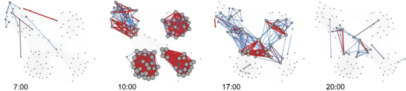
Figure 7: Selected Interactions in the Copenhagen Network Study. Blue edges indicate less frequent interactions, red, more frequent, and vertex size scales with degree (Stopczynski et al., 2014).
ing and subsequent graph representation of the dataset are described in Chapter 4. Specifically, we focus only on the face-to-face contact data. We were provided the interactions of about seven hundred individuals, over one month, reported every five minutes. A selection of those interactions is illustrated by Figure 7. The detail of this contact data gives us the opportunity to simulate transmission of disease with far more granularity, precision, and realism than would be possible in a full mixing model.
We highlight the number of interactions over time in the Copenhagen dataset, plot-ted in Figure 8. We find that not only do individuals make plenty of contact with each other (peaking at almost 1800 interactions within the span of five minutes on the third Monday), but their interactions also occur with a distinctive, immediately recognizable pattern. Every day, the most interactions occur around midday, and there are significantly more on what we infer to be weekdays compared to weekends.
0 200 400 600 800 1000 1200 1400 1600 1800 2000
0 7 14 21 28
Nu m be r of I nt er ac tion s Time (days)
Figure 8: Interactions by Time in the Copenhagen Dataset. Preprocessed
as described in Chapter 4.
0 1 2 3 4 5 6 7 8 9 10 11
1 11 21 31 41 51 61 71 81 91
101 111 121 131 141 151 161 171 181 191 201 211 221 231 241 251 261 271 281 291 301 311 321 331 341 351 361 371 381 391 401 411 421 431 441 451 461 471 481 491
Nu m be r of I nd iv id ual s
Number of Unique Interactions
Chapter 3
RELATED WORKS
As this thesis is concerned with epidemic spreading in social networks that incorporate a richer level of detail, its related works fall broadly into two categories: those that explore epidemics on graphs and those that develop more detailed epidemic models.
3.1 Disease Spreading on Graphs
Although they employed neither a sophisticated epidemiological model nor a particu-larly detailed network, Kephart and White were, in 1991, among the first to propose modeling the spread of a virus using a graph (Kephart & White, 1991). Working to adapt existing mathematical models of infections, they argue that the traditional methods are not quite precise enough when dealing with computer viruses. Un-like their biological counterparts, which, in many cases, can be transmitted via the surrounding environment, computer viruses must generally spread across an active connection between two individual members of the population. It is unreasonable to assume that a computer will routinely interact with every other computer on the network. Compared to the assumptions made by a full mixing model when simulating a biological disease, it is even more unrealistic to assume that an infected computer is equally likely to infect any other computer on the network.
graphs. These simulations allow them to confirm that concepts in traditional epi-demiology can also be applicable to network security: for instance, they show that a perfect defense against malware is not strictly necessary, provided individual infec-tions are detected and corrected quickly enough.
Though their work is groundbreaking, Kephart and White acknowledge that it is overly simplistic and that, at the time, they lacked a sufficient basis of real-world data. They concede that the SIS model represents an extreme situation in which users take no precautions after their computers have been infected for the first time. Their simulations do not consider how the structure of the network might change over time: they do not account for the possibility that a user might disconnect their computer from the network upon discovering the infection.
3.2 Disease Spreading with Mobility Patterns
The incorporation of individual movements, such as we might find in high resolution social networks, is not exclusive to models based on graphs. Granell and Mucha argue that the traditional reaction-diffusion system for modeling the movements of individuals is inadequate when considering diseases that affect humans (Granell & Mucha, 2018). Humans are habitual; they do not diffuse uniformly or randomly.
is verified with a variety of Monte Carlo simulations of situations not based on any particular real-world data.
Similarly, Gemmetto, Barrat, and Cattuto used temporal information to refine a con-ventional epidemic simulation (Gemmetto, Barrat, & Cattuto, 2014). They, however, derived their data from a real-world high resolution contact network obtained from sensors worn by children at a primary school in Lyon, France. Although their work is not explicitly posed as a graph-based problem, their model did separately and in-dividually compute the results of every contact between children as it simulated the spread of an influenza-like disease using SEIR.
Since theirs is a real-world dataset, Gemmetto et al. investigate typical real-world attempts to combat the spread of infections in this situation. Their model allows them to simulate the effects of varying levels of school closure, from canceling just one class to canceling all classes in a grade to closing the entire school temporarily. They are able to show that canceling just one class (the class containing the infected child) can drastically reduce the spread of an infection, and may actually be preferable to closing the entire school — not only do the children in other classes remain productive in school, but they are shielded from any infections spreading through the general community.
3.3 Disease Spreading on Graphs with Mobility Patterns
Combining both mobility data and graph-based simulation, the work of Frías-Martínez, Williamson, and Frías-Martínez more closely resembles that of this thesis: they con-structed and infected a temporal social network of an entire city in Mexico (Frías-Martínez, Williamson, & Frías-(Frías-Martínez, 2011). Their location data was collected from cell towers, so it is not nearly as precise as the wearable sensor data employed by Gemmetto et al. or the data collected in the Copenhagen Network Study, but Frías-Martínezet al. specifically chose a time and place that had been affected by the 2009 H1N1 swine flu pandemic. Their agent-based social network model simulates infections using compartmental SEIR while considering interactions and mobility pat-terns on an individual basis.
By including these real-world mobility patterns in their network, Frías-Martínez et al. could tweak the simulated movements of their population, allowing them to ret-rospectively analyze the effectiveness of the Mexican government’s response to the outbreak. They were able to tentatively show that closing schools within the first week, then prohibiting all non-essential movements within the following week delayed the exponential spread of infections by forty hours and reduced the overall number of cases by10%.
Though they had a different goal, Stopcyznski, Pentland, and Lehmann also infected a high resolution social network — the Copenhagen network (Stopczynski, Pentland, & Lehmann, 2018) (Stopcyznski and Lehmann being two of the researchers behind the Copenhagen Network Study). They considered two networks formed from the same dataset: one including only interactions between individuals that came within
they then randomly sampled long-range interactions to ensure that both networks contained the same number of edges.
By applying an infection with a simple SIR model to these two networks, Stopcyznski et al. are able to emphasize their structural differences (perhaps unsurprisingly, they find that their epidemic is more difficult to contain if it is allowed to spread through long-range interactions). This model is neither based on nor intended to simulate any real-world disease; it was developed only to highlight the differences between the short- and long-range networks.
3.4 Span-Cores in Temporal Networks
Finally, while it is neither exclusively applicable to the task of simulating epidemics nor to the concept of high resolution social networks, the theoretical work of Gal-imberti, Barrat, Bonchi, Cattuto, and Gullo is of tangential interest to this thesis. They introduce the concept of a “span-core”, essentially, a k-core for graphs that change over the course of discrete time steps (Galimberti, Barrat, Bonchi, Cattuto, & Gullo, 2018). The Copenhagen dataset is such a network, and we employ k-cores in Section 4.4.3.
Chapter 4
IMPLEMENTATION
4.1 Preprocessing
Four week’s worth of the Bluetooth-based face-to-face data collected by the Copen-hagen Network Study (Stopczynski et al., 2014) was provided to us in CSV form, an example of which is shown in Table 1. Each Bluetooth scan was given as a quadruple of a timestamp, a “User A ID” (the scanner), a “User B ID” (the scannee), and a Re-ceived Signal Strength Indicator (RSSI). Scans are reported at discrete intervals, and timestamps are integers representing the number of seconds since the start the study. Since scans were reported every five minutes, timestamps begin at 0 and increment by300. A User B ID of “−1” indicates that User A reported scanning no Bluetooth devices at that time, while a User B ID of “−2” indicates that User A scanned a device that was not part of the study.
4.2 Graph Representation
We model the scans of each timestamp as individual undirected, weighted graphs using the iGraph library for Python (The iGraph Core Team, 2015). These individual graphs can collectively be treated as snapshots of a network that changes over time. In each graph Gi = (Vi, Ei), vertices represent users; there is an edge between vertex
u and vertex v of weight w if user u scanned user v or vice versa with RSSI w at timestamp ti. For each vertex v, we further record of the number of external devices
scanned by user v.
We always assume that if user uhas come face-to-face with user v, then userv must have come face-to-face with user u. In some rare situations, the raw data contains both a scan of user u by user v and a scan by user v by user u at time ti. In these
cases, we add only one edge between users u and v, weighting that edge with the higher (closer to zero, indicating a stronger signal) RSSI of the two scans.
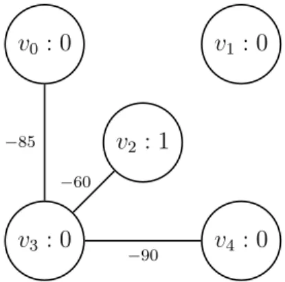
Finally, we observe that not every user is present in a scan in every timestamp. This could simply be because their phone had no power at that time. For the purposes of our simulation, we add vertices to the network once their corresponding users appear in a scan, but we never remove them. Users that have appeared before yet fail to appear in any scan in a later timestamp will be persisted as isolated vertices — since we are interested in simulating the spread of a disease, we need to keep track of users’ states with respect to the infection at all times, regardless of whether or not they successfully report their scanning status. One snapshot that results from parsing the data in Table 1 is shown in Figure 10.
v2 : 1
v0 : 0 v1 : 0
v3 : 0 v4 : 0
−85
−60
−90
Figure 10: Graph Snapshot of One Timestamp. The snapshot produced by
data at time t1 = 300 in Table 1. Note that v1 is presumed to persist from time t0 = 0, although it is missing from the raw Bluetooth data. Note also that v2 is unique in that it has scanned an external device at this time.
Recovering physical characteristics of interactions (distance between users, for exam-ple) would require that we have specific details of the scanning devices. Since we do not have these details, we assume that face-to-face interaction is binary. The same is true of the number of external devices scanned: while we had initially hoped that these scans could be interpreted as contacts with individuals who did not participate in the study, there is not necessarily any correlation between external devices scanned and number of face-to-face interactions. “External devices” includes wireless mice, for example, not just other phones (Sapieżyński, n.d.). So, although this information is represented in our graph as attributes of each vertex, none of our simulations make use of it.
users formed a line when they came into contact with each other, such that user b was close enough to scan both users a and c, but those users were not close enough to scan each other.
4.3 Simulation Architecture
We developed a modular system that allows the definition of compartmental models in Python. Each model is defined within a Python module and implements, at minimum, three functions: one to initialize new vertices when they are first added to the network, one to log information about the current state of the model, and one that simulates the spread of disease for a single timestep.
This architecture allows us easily develop and swap out variations of models for different diseases and different amounts of simulation complexity. For any time ti,
the individual model modules are given full access to the iGraph vertices of both the Gi and Gi+1 snapshots, so they may adjust the attributes contained within as necessary — the times at which individuals enter each compartment, for instance, are stored as attributes of their corresponding vertices.
4.3.1 The Flu Model
1918 outbreak is estimated to have killed 50 million people worldwide (Johnson & Mueller, 2002), easily more than twice the total casualties of World War I, which ended that same year (Gilbert, 1994). The flu is typically transmitted by airborne particles released by a nearby infected individual’s coughing or sneezing.
While flu vaccines exist, the rapid mutation of the flu families of viruses prevents humans from developing any long-term immunity; roughly every year, they must reacquire (whether by vaccination or by recovery from infection) immunity to new strains of the virus (Krammer et al., 2018). Since our dataset only covers a month of interactions, our simulations do not run long enough for this lack of long-term immunity to have any effect. Therefore, we chose to simulate the flu with a simple SIR model: unless otherwise specified, individuals begin the simulation susceptible to infection. If infected, they immediately become infected and infectious for between5 and 8 days, after which they are considered to be completely recovered.
In the case of the 1918 Spanish flu, the basic reproduction number has been es-timated as R0 ∈ [2,3] (Mills, Robins, & Lipsitch, 2004). On the first Monday of the Copenhagen Network study, individuals made contact with an average of 28.18 other participants. We thus estimate the transmission probability per contact as β = 28.218.5×6 = 0.015. This is a crude estimate at best. Notably, an individual in the Copenhagen dataset does not necessarily make equal or singular amounts of contact with those28.18others. We reiterate that this simulation is only intended to validate our software architecture and establish that epidemic outbreaks are possible in the network. The interventions which we will apply in Section 4.4 are not based on such rough estimates.
next by default, though they may be infected later in the simulation of this timestep. Whenever an individual is infected, they are moved to the infected state in the next snapshot and assigned a random infectious period between 5 and 8 days. If an indi-vidual was previously in the infected state, and their infectious time has expired in the intervening five minutes, then they are moved to the recovered state. If, however, an infected individual is scheduled to remain infectious, we explore all of its neighbors in the previous snapshot, infecting any susceptible neighbors with probability 0.015. Finally, recovered individuals remain in the recovered state; as previously noted, our simulation would not run long enough for them to realistically move back into the susceptible state.
All of these model parameters are uniformly applied to every individual in the pop-ulation, an assumption that is also true of our forthcoming measles and norovirus models. For example, we do not attempt to simulate other pre-existing conditions that could exacerbate a flu infection. We do not have enough demographic informa-tion to simulate otherwise. That being said, real-world populainforma-tions similar to that of the Copenhagen Network Study should, in fact, be composed primarily of healthy individuals around the same age.
4.3.2 The Measles Model
to spread effectively even when less than 10% of the population is at risk — in other words, its herd immunity threshold is at least 90% (Rota et al., 2016).
Once it infects its host, the measles virus incubates for 10–12 days (CDC (Centers for Disease Control and Prevention), n.d.-e). Prodrome, an initial period of milder symptoms, then lasts 2–4 days, followed by a rash that lasts 5–6 days, and the host will be contagious for up to 4 days before and after the rash appears. All told, an infectious individual will spend up to 14 days infecting up to 90% of those they meet. Thus, it is not surprising that measles has been targeted by the World Health Organization for elimination, though their 2015 global target for reduction in cases was not met (Rota et al., 2016).
We model measles using an SEIR compartmental model. Individuals begin in the susceptible state. Once infected, according to the timeline enumerated above, they are in the exposed state for between 10and 12 days, then move to the infected state for 7 to 14 days. Individuals are only capable of transmitting the disease while in the infected state, which they do so at a rate per contact of β= 0.90(CDC (Centers for Disease Control and Prevention), n.d.-e). As with influenza, those infected with measles eventually move to the recovered state, after which they are no longer at risk of being infected. While measles carries a non-zero chance of death or other complications (Rota et al., 2016), we chose not to simulate any of these alternative outcomes.
capable of spreading rapidly by face-to-face transmission alone. We also note that this possibility would not be simulatable with traditional full-mixing models, either.
4.3.3 The Norovirus Model
To demonstrate the flexibility of our architecture beyond simple compartments and face-to-face contact events, we implemented a model to simulate the spread of norovirus, the most common foodborne disease in the United States (CDC (Centers for Disease Control and Prevention), n.d.-d). Because norovirus is easily spread by contaminated food, by vomiting, and by toilet flushing, we believe that some amount of location-based information is essential to a realistic simulation model. In lieu of any such empirical data provided to us from the Copenhagen Network Study, we implemented a compartmental model that also conservatively identifies clusters of individuals in close contact with one another.
Ideally, we would be able to take the entire month’s worth of snapshots, compute the connected components of each, and attempt to track patterns of how vertices enter and exit components. This would allow us to estimate exactly when a cluster formed, and it could allow us to smooth over any potential hiccups in the reported data — if an individual remained in a cluster consistently but lost phone power for ten minutes during that time, for instance.
simu-t1 : v1 v0 v2 v4 v3 v5
t2 :
v1 v0 v2 v4 v3 v5
t3 :
v1 v0 v2 v4 v3 v5 v6
t4 :
v1 v0 v2 v4 v3 v5 v6
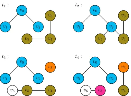
Figure 11: Cluster Detection over Four Snapshots. Note that v6 is never
considered, as it cannot be in any non-trivial cluster.
late the spread of norovirus among the individuals of a cluster with some alternative probability of transmission. Assuming our clustering interval is relatively short, on the order of hours, any individuals newly infected by this method would not have time to themselves spread the infection, so we do not need to retroactively explore their interactions with individuals outside the cluster. Importantly, this allows our model to identify clusters in a streaming fashion. At any given timestep, it need only consider the next snapshot and the existing clusters that it has computed up through the previous snapshot: if a vertex v belonged to cluster C at time ti, andv belongs
to component A at time ti+1, then v belongs to cluster C∩A at timeti+1.
v5, so their cluster is split in two. Note that the choice to color v3’s cluster orange whilev4 and v5’s remains olive green is entirely arbitrary, and there is no significance within our model to which vertices “remain” in an existing cluster and which are “split off”. Finally, at timet4, the lack of an edge between v5 and v4 splits the former off into an fourth cluster. Note that although an edge between v3 and v4 appears at time t4, those vertices are not placed in the same cluster; they have been irrevocably separated into different clusters at time t3. Also note that v6 is not placed into any cluster at all, although it always appears in the same connected component as v5. Since it does not appear in the initial snapshot, it cannot possibly appear in the same connected component as any other vertex in all snapshots. It cannot appear in any meaningful cluster, so, for the purposes of our model, it can be ignored.
Similar to influenza, immunity to norovirus is not permanent, but lasts long enough that individuals cannot be infected more than once within the time span of our simu-lations. We therefore simulate norovirus using an SEIR compartmental model, just as we did measles. Recent work based on reported outbreaks in Japan has estimated the basic reproduction number of norovirus to be R0 ∈ [1.11,4.15] (Matsuyama, Miura, & Nishiura, 2017). Adopting the same crude estimation as we did for influenza, this gives our model a transmission probability per contact ofβ = 282.18.63×2 = 0.047. While it may be possible for individuals to continue spreading the disease at some lower rate once recovered (CDC (Centers for Disease Control and Prevention), n.d.-d), we did not model this possibility. Individuals remain in the exposed state for 0.5 to2 days, and in the infected state for 1to 3days.
noon and 1:00pm, and between 1:00pm and 2:00pm. We assume that these individu-als either share a dormitory or a meal with each other. Within each of these groups, every infected individual has the opportunity to spread the infection to everyone else in the cluster. This differs from the normal simulated mode of transmission in two ways: firstly, this potentially gives infected individuals far more influence over those nearby. Consider, for example, the clusters given by the four snapshots in Figure 11. Suppose that, in this situation, individual v1 was infected. Since v1 appears in the same cluster as v0 and v2, it would have a chance to infect both of those individu-als. Notice, however, that v1 never makes direct face-to-face contact with v2. In the standard simulation, the infection would not be able to spread to v2 within the time span of these four snapshots. In the standard simulation, v1 could potentially infect v0, but v0 would not become contagious quickly enough to then infectv2.
Additionally, we can apply an alternative probability of transmission to the con-tact events assumed to have taken place within a cluster. In a food service sce-nario, a single infectious employee who continued to work while symptomatic but took reasonable precautions (wearing gloves and frequently washing or disinfecting hands) was estimated to infect 167.4 customers over 2000 servings, where 80% of the population was susceptible (Duret et al., 2017). Assuming that no customer was served twice, this gives an increased transmission probability per cluster contact of βcluster = 0.8167×2000.4 = 0.1046.
4.4 Interventions
in-tensified effort to contain the disease in 1966, the last naturally occurring case was reported in Somalia in 1977, and smallpox was declared eradicated in 1980 (Fenner et al., 1988). The primary plan was a mass vaccination campaign with a goal of immunizing 80% of the global population. Additionally, the WHO established an extensive surveillance program to preempt outbreaks: whenever a case was reported, the infected person would be isolated and their household and close contacts would be vaccinated, a strategy termed “ring vaccination”. This sort of targeted intervention could not be simulated in a full mixing model, which does not distinguish between the individual members of each compartment and their interactions.
Compared to traditional full mixing, our graph-based models give us far more control over the granularity of the simulation. They allow us to explore the transmission of a disease on an individual, per-contact basis. They also allow us to implement more sophisticated simulations based on the structure of the network, as we did with norovirus. And, as a result of their more fine-grained simulation, graph-based models also enable additional opportunities to explore interventions: strategies for preventing or containing an epidemic.
we must account for ineffective vaccinations. Finally, at the time of this writing, measles outbreaks in the United States have recently risen drastically (CDC (Centers for Disease Control and Prevention), n.d.-b), so interventions that target measles are of greater immediate relevance. A summary of interventions is given in Table 2.
4.4.1 Uniform Vaccination
Our baseline intervention is vaccination with uniform probability. Whenever a indi-vidual first appears in Copenhagen Network Study — whenever a new vertex is added to the network — that individual has a chance of gaining complete immunity to the disease. Effectively, individuals start in the recovered state instead of in the suscep-tible state with some probability p. We simulated varying amounts of vaccination, fromp= 0.05top= 0.95in increments of 0.05.
4.4.2 Vaccination by Degree Distribution
Considering our lack of demographic information, vaccination with uniform proba-bility is likely the most realistic preventative intervention we can employ. However, we imagine a scenario where there are a limited number of vaccines. Perhaps the vaccine is costly to manufacture, difficult to administer, or experimental in nature. Perhaps we are not dealing with measles proper, but with a new disease that spreads similarly to measles. In these situations, rather than randomly selecting individuals to vaccinate, we would like to vaccinate those that have the greatest effect on the spread of the infection.
v0
v1
v2
v3 v4
v5 v6
v7
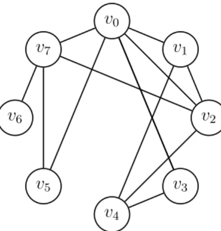
Figure 12: Example Degree Distribution. This graph has degree distribution
(0,1,2,2,2,1)
vertex. Alternatively, vaccinating an individual effectively removes their vertex from the network: the individual is simply no longer capable of affecting the spread of the infection. If we are to contain an infection by removing a limited number of vertices, and the infection spreads along edges, then our ultimate goal is to remove vertices in order to disconnect the network into multiple connected components. If we can split the network into multiple connected components, any infection that begins in one component will not be able to spread to the others. Given this goal, if we have a limited number of vaccinations, one possible approach is to vaccinate those individuals who make the most contact with other individuals.
The degree distribution of a graph is simply the numbers of vertices having each of the possible degrees. For example, the graph in Figure 12 has degree distribution (0,1,2,2,2,1), because there are zero vertices with degree 0, one vertex with degree
1, two vertices with degree2, two vertices with degree 3, two vertices with degree4, and one vertex with degree5. Alternatively, we could express the degree distribution as a sequence of bins of vertices: (∅,{v6},{v3, v5},{v1, v4},{v2, v7},{v0}).
re-v1
v0
v2 v4 v3
v5 v6
Figure 13: Example Flattened Graph. Flattening the four snapshots in Figure
11 produces this graph.
sponsible for connecting more components together, we simulated the vaccination of limited numbers of individuals, prioritizing those of highest degree. Effectively, this is simply sorting the vertices in ascending order by degree and vaccinating the last λ corresponding individuals. For some values of λ, this will be close if not identical to vaccinating the individuals in the k highest bins of the degree distribution.
The network representing the Copenhagen Network Study, however, is not a single graph; it is composed of numerous graph snapshots. Before we can compute the degree distribution, we must decide how many snapshots to “flatten” into a single graph. Given a sequence of snapshots, the flattened graph contains an edge between verticesu and v if and only if there is an edge betweenu and v in at least one of the snapshots. The result of flattening the four snapshots in Figure 11 is shown in Figure 13.
v0
v1 v2
v3
v4 v5
Figure 14: Example k-Cores. This graph’s highest k-core does not include its
highest degree vertices.
In all three cases, we simulated varying numbers of vaccinations in increments of 10. There are, for instance, 659 unique individuals seen in the first week of the Copenhagen Network Study. We therefore simulated administering λ vaccinations, where λ ∈ {10,20,30, . . . ,650}, and the vaccinations were given to the λ vertices of highest degree based on the flattened graph of the first week.
4.4.3 Vaccination by k-Cores
With the same reasoning that motivated vaccination by degree, we next investigated vaccination informed by k-cores. A k-core is a maximal subgraph such that every
Vertices belonging to higher k-cores roughly correspond to vertices in denser regions of the network, thus, we consider the possibility that these individuals have a greater effect on the spread of an infection. As we did with the degree distribution, we first considered three methods of flattening the network: flattening the entire month’s snapshots, flattening the first week, and flattening the first Monday. For each flat-tened graph, we computed everyk-core. Given each set ofk-cores, we then simulated limited numbers of vaccinations, and vaccinations were given to the individuals that appeared in the highest cores.
4.4.4 Vaccination by Density Decomposition
Similar tok-cores, the density decomposition partitions the vertices of a graph based on the density of their subgraphs, producing “rings” of vertices (Borradaile, Migler, & Wilfong, 2018). Compared to the highest core, the highest ring better approximates the densest subgraph. It can be shown that if the highest ring in the density decompo-sition is Rk, then the density of the densest subgraph is in the range(k−1, k], where
density is the ratio of edges to vertices. Furthermore, every vertex in the densest subgraph must be in the highest ring.
The downside to the density decomposition is its computational complexity. Finding the density decomposition involves first finding an “egalitarian orientation”. Finding that orientation has a running time of O(|E|2), which is the lower bound on the running time of the decomposition. The k-cores of a graph, in contrast, can easily be found all at once with a simple, greedy, pruning algorithm in linear, O(|V|+|E|) time (Matula & Beck, 1983).
to propagate the infection. The density decomposition was separately computed for the network flattened over the first Monday, over the first week, and over the entire month. For each decomposition, we simulated vaccinating a limited number of individuals drawn from the highest rings.
4.4.5 Quarantining
The interventions we have considered thus far all revolve around vaccination. They all rely on the concept of inducing immunity to a disease before coming into contact with an infectious individual. If an individual has already been infected, an alternative method of preventing an epidemic is to quarantine that individual: to isolate them so that they cannot spread the infection to others. Effectively, this involves augmenting our SEIR measles model to produce an SEIQR model, where individuals enter a quarantined state between the infected and recovered states. Such a compartmental model has previously been used to explore the impact of isolation on seasonal patterns of infections (Feng & Thieme, 1995).
4.5 Summary of Simulations
timestamp user_a user_b rssi
0 0 1 -90
0 2 -1 0
300 0 3 -85
300 2 3 -80
300 2 -2 -70
300 3 2 -60
300 4 3 -90
Chapter 5
METHODOLOGY
In all simulations, one individual was randomly chosen from the first snapshot to be the “seed” (not to be confused with the seed of the random number generator) of the infection. Though it may not be realistic, for the purposes of our simulations, participants of the Copenhagen network study are assumed to make negligible contact with the outside world, and we do not simulate any chance of infection via such external contacts. In order to allow ample time for infections to run their course, the dataset, preprocessed as described in Section 4.1, was looped twice, creating eight weeks of individual contact events. A summary of scenarios simulated is shown in Table 3.
5.1 Baseline Models
Each model — SIR influenza, SEIR measles, and SEIR norovirus — was first simu-lated without any interventions. For each baseline model,30seeds (in both senses of the word: we tested different seeds of infection; to keep them consistent across trials, we set the seed of the random number generator) were tried, and for each seed, 5 simulations were run. Thus, in total, 150 simulations were run for each model, 450 overall.
the influenza model, or one who is or has been in the exposed or infected states, in the cases of the measles and norovirus models.
5.2 Models with Interventions
As noted in Section 4.4, all of our interventions were tested based on the measles model. For uniform vaccination, we simulated varying values of the vaccination prob-ability p from p = 0.05 to p = 0.95, in increments of 0.05. For each value of p, we tested 10 different seeds for the initializing random number generator, and for each seed, we ran 5 simulations — while the random number generator is seeded when determining which individuals are initially vaccinated or infected, it is not when de-termining transmission of infection. In total,950simulations were run for the uniform vaccination scenario.
For the degree-, core-, and ring-based vaccination scenarios, we vaccinated λ indi-viduals whose vertices were among those with the highest degree, core, or ring. The values of λ were varied in increments of 10up to the total number of vertices in the corresponding flattened graphs. In the event of a tie between vertices, vaccinations were distributed randomly. For example, suppose that there were 20 vertices in the highest ring, ring Rk, and 30 vertices in Rk−1. If n = 30, we would vaccinate the 20 vertices in ring Rk along with 10 vertices randomly selected from Rk−1. If we then incremented to n = 40, we would vaccinate the same 20 vertices in ring Rk, and we
would make a new random selection of20 vertices from Rk−1.
first appeared in the dataset. That is to say, in the uniform vaccination simulations, every individual is vaccinated with some probability p once they make their first appearance, even if that is not in the first snapshot. Likewise, in the degree-, core-, and ring-based simulations, selected individuals were vaccinated once they made their first appearance, even if that was not in the first snapshot. Additionally, because some individuals first appear in later snapshots, it is possible that the λ vertices of highest degree, core, or ring encompass all of the vertices in the first snapshot. In this situation — which is also theoretically possible with uniform vaccination, though highly improbable — it is not possible to seed the infection during the first timestep, so we continue attempting to infect individuals as they make their first appearances until we find a valid seed.
Specifically, there are612individuals who appear during the first Monday,659during the first week, and 692 over the entire month. For each value of λ, we ran 5 simula-tions. Thus, the61varying values of λfor the first Monday,65for the first week, and 69 for the first month collectively mandate 2925 simulations for the degree-, core-, and ring-based scenarios.
Scenario Varying Parameters Total Simulations
Baseline Influenza 30 seeds 150
Baseline Measles 30 seeds 150
Baseline Norovirus 30 seeds 150
Uniform Vaccination 19 values ofp 950
10 seeds
61values of λ(Monday) 305
Vaccination
by Degree 65 values ofλ(week) 325
69values of λ(month) 345
61values of λ(Monday) 305
Vaccination
by k-Core 65 values ofλ(week) 325
69values of λ(month) 345
61values of λ(Monday) 305
Vaccination
by Ring 65 values ofλ(week) 325
69values of λ(month) 345
Quarantine 2 values ofp 300
30 seeds
total 4625
Chapter 6
RESULTS
6.1 Baseline Scenarios
We begin by infecting the Copenhagen network using our three basic models. This serves to confirm that our models are functional, to establish that an epidemic out-break is possible, and to provide a baseline against which to compare the efficacy of our eventual attempted interventions.
6.1.1 Influenza
We first consider a single baseline influenza scenario, illustrated by Figure 15. Here, we have randomly selected a single seed for the infection, then run five simulations based on that starting situation. In other words, while the randomly chosen seed was held constant in all five simulations, the individual transmission events were not.
0 100 200 300 400 500 600 700
1 7 49
Nu
m
be
r
of
Af
fe
ct
ed
I
nd
iv
id
ual
s
Time (days)
Figure 15: Affected Individuals in a Baseline Influenza Scenario. Five
in-fluenza simulations used the same initial seed of the infection. Note the logarithmic scale for time to better illustrate the individual curves.
These effects are reflected in the plot of infected individuals, Figure 17. In most simulations, the number of currently infected individuals reaches its peak by the beginning of the second week, but there are two where the curve is shifted to the right by one week. We also note the difference in the general shape of the curves to the left and to the right of the peak: because we simulate transmission of disease through individual contact events that occur with some daily pattern, the increasing portion of the curve is noticeably stepped. However, once an individual is infected, we roll a die with regards to when they will recover, and this randomness smooths out the decreasing portion of the curve.
0 100 200 300 400 500 600 700
0 7 14 21 28 35 42 49 56
Nu m be r of Af fe ct ed I nd iv id ual s Time (days)
Figure 16: Affected Individuals in Baseline Influenza Scenarios. Each curve
is an average of five simulations with the same infection seed and no interventions; the pointwise median of thirty curves is shown in black.
0 100 200 300 400 500 600 700
0 7 14 21 28 35 42 49 56
Nu m be r of I nf ec te d In di vi du al s Time (days)
Figure 17: Infected Individuals in Baseline Influenza Scenarios. Each curve
state; they are immediately capable of passing on the infection. Thus, the plotted curves begin to show unencumbered, exponential growth within the first couple of days.
6.1.2 Measles
In contrast to the immediate dispersal of influenza, the measles virus spreads with a more complex pattern, as shown in Figure 18. Because the measles model uses the additional exposed state, and exposed individuals cannot transmit the disease, the outbreak initially appears to slow after infecting about a hundred individuals — certainly, it spreads more slowly than our influenza simulations. In reality, however, these are just the individuals that the original seed is capable of directly infecting. The outbreak is initially limited by the number of individuals with whom that seed makes direct contact. The incubation period of measles is between10and12days, so by day12, the initial batch of exposed individuals start transitioning into the infected state, and only then can the epidemic truly spread.
This behavior is more evident in Figure 19, where we plot the number of exposed individuals in blue alongside that of infected individuals in red. Up until about day 10, the initial seed is the only individual capable of spreading the disease, and the distinctive stepped shape of the exposed curves reflects that seed’s daily movement patterns. Notably, the infection spreads more slowly on days 7 and 8, which are weekends. Much more rapid growth of the exposed curves begins around day 12, at the same time we begin to see growth of the infected curves.
0 100 200 300 400 500 600 700
0 7 14 21 28 35 42 49 56
Nu
m
be
r
of
Af
fe
ct
ed
I
nd
iv
id
ual
s
Time (days)
Figure 18: Affected Individuals in Baseline Measles Scenarios. Each curve
is an average of five simulations with the same infection seed and no interventions; the pointwise median of thirty curves is shown in black.
as previously shown in Figure 18, but the peaks of the exposed and infected curves in Figure 19 do not get nearly so high. This is because the affected individuals are split between the exposed and infected states; they are never all in the same compartment at the same time. For the sake of completeness and later comparison, the sizes of all compartments for five individual simulations are presented in Figure 20.
6.1.3 Norovirus
0 100 200 300 400 500 600 700
0 7 14 21 28 35 42 49 56
Nu m be r of E xp os ed /I nf ec te d In di vi du al s Time (days) Exposed Infected
Figure 19: Exposed and Infected Individuals in Baseline Measles Scenarios. Each curve is an average of five simulations with the same seed and no interventions; the median of thirty curves is shown in black.
0 100 200 300 400 500 600 700
0 7 14 21 28 35 42 49 56
Nu m be r of I nd iv id ual s Time (days) Susceptible Exposed Infected Recovered Affected
Figure 20: SEIR Compartments in a Baseline Measles Scenario. Five
0 100 200 300 400 500 600 700
0 7 14 21 28 35 42 49 56
Nu m be r of Af fe ct ed I nd iv id ual s Time (days)
Figure 21: Affected Individuals in Baseline Norovirus Scenarios. Each curve
is an average of five simulations with the same infection seed; the pointwise median of thirty curves is shown in black.
0 100 200 300 400 500 600 700
0 7 14 21 28 35 42 49 56
Nu m be r of E xp os ed /I nf ec te d In di vi du al s Time (days) Exposed Infected
Figure 22: Exposed and Infected Individuals in Baseline Norovirus
Sce-narios. Each curve is an average of five simulations with the same seed; the median
model must pass through an exposed state before they can spread the disease, but that period is short enough for exponential growth to begin within a couple days, in similar fashion to the overly-simplistic flu simulation. Individuals also spend relatively little time in the infected state; the end result is that the exposed and susceptible curves of norovirus simulations rise and fall in rapid, overlapping spikes. Individuals quickly become exposed, transition to the infected state, infect others, and recover. As shown in Figure 22, the numbers of individuals in each compartment never reach the heights they do in flu or measles simulations, but as shown in Figure 21, the outbreak still affects the majority of the population.
6.2 Uniform Vaccination
In the uniform vaccination scenarios, individuals are placed in the recovered state instead of the susceptible state with some probability p upon their first appearance in the dataset. One selected example is shown in Figure 23. In this simulation, we set p = 0.90. Of the vaccination probabilities we tested, this most closely matches the vaccinated percentage of the population in the United States as of 2017 (CDC (Centers for Disease Control and Prevention), n.d.-a). The total number of individuals who have been affected by the disease is plotted in black. Though dramatically subdued compared to the baseline curve in Figure 20, this curve exhibits a period of faster-than-linear growth, and it flattens out as it approaches the maximum number of susceptible individuals, indicating that almost every susceptible individual has already been infected.
0 100 200 300 400 500 600 700
0 7 14 21 28 35 42 49 56
Nu
m
be
r
of
I
nd
iv
id
ual
s
Time (days)
Susceptible Exposed Infected Recovered Affected
Figure 23: SEIR Compartments in a Uniform Vaccination Scenario. Five uniform vaccination simulations used the same initial seed, where p = 0.90. maxt{|St|}= 73; mint{|St|}= 5; maxt{|At|}= 74.
For each probability, we tested 10different infection seeds, and for each seed, we ran 5simulations. Thus, each curve in Figure 24 represents the median of 10averages of 5 simulations each. As illustrated by the shapes of the curves, increasing the proba-bility of vaccination neither alters nor delays the general pattern of the outbreak, it merely places a cap on the number of individuals that can eventually be infected.
Copen-0 100 200 300 400 500 600 700 0 100 200 300 400 500 600 700
0 7 14 21 28 35 42 49 56
Nu m be r of Af fe ct ed I nd iv id ual s Time (days) p = 0.10
p = 0.20 p = 0.30 p = 0.40 p = 0.50 p = 0.60 p = 0.70 p = 0.80 p = 0.90
Figure 24: Affected Individuals in Uniform Vaccination Scenarios. Each
line is the median of ten averages of five simulations each (ten infection seeds, five simulations per seed).
0 100 200 300 400 500 600 700
0.05 0.1 0.15 0.2 0.25 0.3 0.35 0.4 0.45 0.5 0.55 0.6 0.65 0.7 0.75 0.8 0.85 0.9 0.95
Nu m be r of Af fe ct ed I nd iv id ual s
Probability of Vaccination, p
Figure 25: Summary of Uniform Vaccination Scenarios. Each box
hagen network, the herd immunity threshold (typically estimated between 89% and 94% (Rota et al., 2016)) appears to be higher than95% in our simulations.
The only noticeable outlier occurs atp= 0.75: in this simulation, by random chance, we happened to vaccinate every individual immediately surrounding the one who would eventually be chosen as the seed of the infection, so the infection was never able to spread. This inadvertent targeted ring vaccination is, of course, the exception, not the trend.
6.3 Targeted Vaccination
We now imagine a hypothetical scenario in which we have a limited number of vaccines to distribute in preparation for an epidemic. In such a situation, we would like to try to target individuals for immunization in a more intelligent manner than uniform random vaccination.
6.3.1 Vaccination by Degree
We first simulated prioritizing individuals by the degrees of their vertices: in other words, those who made more unique contacts would receive the vaccine first. The results of this intervention are given by Figure 26. As detailed in Section 4.4.2, we tested three ways of computing the degree of each vertex in this network that changes over time. The simulation in the top-left of Figure 26 computes the degree based on the first Monday; in the top-right, based on the first week; in the center, based on the entire month.
0 100 200 300 400 500 600 700 0 100 200 300 400 500 600 700
0 7 14 21 28 35 42 49 56
Number of Affected Individuals
Time (days) λ = 10
λ = 100 λ = 200 λ = 300 λ = 400 λ = 500 λ = 600
0 100 200 300 400 500 600 700 0 100 200 300 400 500 600 700
0 7 14 21 28 35 42 49 56
Number of Affected Individuals
Time (days) λ = 10
λ = 100 λ = 200 λ = 300 λ = 400 λ = 500 λ = 600
0 100 200 300 400 500 600 700 0 100 200 300 400 500 600 700
0 7 14 21 28 35 42 49 56
Number of Affected Individuals
Time (days)
λ = 10
λ = 100
λ = 200
λ = 300
λ = 400
λ = 500
λ = 540
Figure 26: Affected Individuals when Vaccinated by Degree. Each curve is
the median of five differently seeded simulations withλ vaccinations. Clockwise from top left: degrees computed from one Monday, from one week, and from one month.
find that around λ = 540, the disease no longer infects the majority of susceptible individuals (540 vaccinated, thus,152susceptible, and a median of only28infected). In other words, the herd immunity threshold has been lowered to around 80% — a remarkable improvement over uniform vaccination.
6.3.2 Vaccination by k-Core
Our second targeted vaccination strategy involves the use of k-cores. As with vac-cination by degree, we simulated administering a limited number of vacvac-cinations, prioritizing individuals whose vertices were in higher cores, and we computed those cores based on the first Monday, the first week, and the entire month. These results are shown in Figure 27.
Disappointingly, we find that vaccination by k-core does not appear to perform any better than uniform random vaccination. In retrospect, however, this makes sense: higherk-cores identify subgraphs that are clique-like, whereas higher degrees identify the centers of subgraphs that are star-like. In a social network, we find it believable that there are more stars than cliques. Moreover, k-cores identify denser regions of a graph; they approximately identify clusters of vertices. In a targeted vaccination scenario, we do not necessarily want to vaccinate the clusters of individuals themselves — we want to vaccinate the individuals who connect those clusters to each other.
6.3.3 Vaccination by Ring