arXiv:1602.09014v1 [astro-ph.HE] 29 Feb 2016
GRB 141221A: gone is the wind
O. Bardho
1,2, B. Gendre
3,4,1, A. Rossi
2, L. Amati
2, J. Haislip
5, A. Klotz
6E. Palazzi
2, D. Reichart
5, A. S. Trotter
5,7, M. Bo¨
er
1⋆1ARTEMIS, CNRS UMR 5270, Universit´e Cˆote d’Azur, Observatoire de la Cˆote d’Azur,
boulevard de l’Observatoire, CS 34229, F-06304 Nice Cedex 04, France 2IASF Bologna-INAF, via P. Gobetti 101, Bologna, Italy
3Etelman Observatory, St Thomas, Virgin Islands, USA
4University of the Virgin Islands, 2 John Brewer’s Bay Road, 00802 st Thomas, Virgin Islands, USA
5Department of Physics and Astronomy, University of North Carolina at Chapel Hill, Campus Box 3255, Chapel Hill, NC 27599, USA 6IRAP, CNRS, Universit´e de Toulouse, 9 avenue du colonel Roche, 31028 Toulouse Cedex 4, France
7Department of Physics, NC A&T State University, 1601 E. Market St, Greensboro, NC 27411, USA
Received– Accepted
ABSTRACT
GRB 141221A was observed from infrared to soft gamma-ray bands. Here, we investi-gate its properties, in light of the standard model. We find that the optical light curve of the afterglow of this burst presents an unusual steep/quick rise. The broad band spectral energy distribution taken near the maximum of the optical emission presents either a thermal component or a spectral break. In the former case, the properties of the afterglow are then very unusual, but could explain the lack of apparent jet breaks in the Swift light curves. In the latter case, the afterglow properties of this burst are more usual, and we can see in the light curves the passing through of the injection and cooling frequencies within the optical bands, not masked by a reverse shock. This model also excludes the presence of a stellar wind, challenging either the stellar pro-genitor properties, or the very stellar nature of the propro-genitor itself. In all cases, this burst may be a part of a Rosetta stone that could help to explain some of the most striking features discovered by Swift during the last ten years.
Key words: Gamma-ray:bursts
1 INTRODUCTION
Since the launch of theSwiftsatellite in 2004 (Gehrels et al.
2004), hundreds of gamma-ray bursts (GRB, see Kumar & Zhang 2015, for a review) have been detected, localized and followed both on-board and by telescopes on the ground. This led to a very large sample of events presenting virtually all possible aspects of the standard
model (see Rees & M´esz´aros 1992; M´esz´aros & Rees 1997;
Panaitescu et al. 1998, for a complete description of the model). Several events have been followed in optical with rapid robotic telescopes while the prompt emission was still active or recently concluded, and in a fair number of cases a rising behavior has been observed in this band (see for
instanceGendre et al. 2012).
This rise of the optical wavelength emission can be un-derstood in two different ways: either it is the initial part of the forward shock, which can be observed until the injection
frequencyνmcrosses the observational band, or we see the
⋆ Corresponding author: [email protected]
signature of the reverse shock (e.g.Sari & Piran 1999). Both
phenomena can be interleaved, complicating the analysis.
GRB 141221A is one of these ”optically rising” bursts.
It was detected by Swift at 08:07:10 UT (hereafter T0)
on December 21, 2014 (Sonbas et al. 2014a). The
dura-tion of the burst, while not excepdura-tional (T90 = 36.9± 4.0
s, Ukwatta et al. 2014), allowed the TAROT and Skynet robotic observatories to start the observation while the prompt emission was still active. While in other cases the rise was smooth and not extreme, in this case the optical emission increased very quickly and presented other features usually not seen; the purpose of this work is to investigate those features.
In Section2we present the data for this event. We
ex-plain the data reduction in Section3, and present the
spec-tral and temporal analyses in Section4. We then discuss our
results in Section5, before concluding.
In the remainder of this paper, all errors are quoted at the 90% confidence level (except when otherwise stated),
= 70 km s−1Mpc−1, Ω
m= 0.3 and ΩΛ= 0.73. We will use
the standard notationFν∝t−αν−β.
2 OBSERVATIONS 2.1 High Energy data
Swift-BAT and Fermi GBM: GRB 141221A triggered
both instruments (Ukwatta et al. 2014; Yu H.F. 2014), at
nearly the same time (08:07:10 UT for Swift, 08:07:11.22 UT for Fermi). The recorded duration is, however, longer in the BAT compared to GBM (23.8 s), as one can expect from the larger effective area (and hence better sensitivity)
of BAT/Swift.
Swift-XRT: The XRT observed the burst position
be-tween T0 + 64 s andT0 + 34.9 ks (Beardmore et al. 2014;
Maselli et al. 2014), mostly in PC mode. The afterglow was clearly detected in X-rays.
2.2 Optical and infrared data
Table2presents a log of the observations and the data from
the instruments that are used in this work.Swift-UVOT:
The observations started T0 + 84 s (Marshall & Sonbas
2014). The afterglow is clearly detected.
TAROT La Silla: The observations at TAROT-La
Silla (Bo¨er et al. 2003) started atT0 + 31.2 s and lasted for
about 41 minutes, until the beginning of sunrise (Klotz et al. 2014). The burst is not detected between 31 s and 68 s, with
a limiting magnitudeRlim= 16.6. After that time, the burst
is clearly detected for the remainder of the observation.
Skynet PROMPT-CTIO: The observations with Skynet PROMPT-CTIO (two 14” telescopes), at Cerro
Tololo, Chile (Reichart et al. 2005), started at T0 + 45 s
and lasted for 27.25 m (Trotter et al. 2014a,b). Forty-four exposures were taken in the V and I bands, ranging from 5s to 160s. The optical afterglow was clearly detected with a rising light curve at t = 2 min and peaks at I = 14.8. Skynet
observed the afterglow again atT0+ 23.0 h for 1.5 h, taking
64 exposures of 160s each in V and I bands.
GROND: GROND (Greiner et al. 2008) observations
started atT0+ 142s (Schweyer et al. 2014), and continued
for 18 minutes. The afterglow was clearly detected.
KECK II telescope: Spectroscopic observations with
the Keck II telescope were performed fromT0+ 1.78 h toT0
+ 2.15 h. Several lines were detected (Mg II doublet and Fe II), putting this burst at a redshift of z = 1.452 (Perley et al. 2014).
3 DATA REDUCTION 3.1 Optical/IR data
The TAROT data were reduced using the standard
proce-dure already discussed inKlotz et al.(2008). We converted
the observed signal from the clear filter to the R filter by calibrating the magnitude of the afterglow against nearby stars of similar color.
Subsets of the Skynet images were stacked to maximize the signal-to-noise ratio. Calibration of these images was performed using three stars in the field from the AAVSO
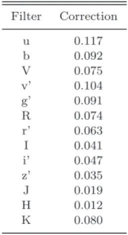
Table 1.Corrections to magnitudes due to Galactic extinction.
Filter Correction
u 0.117
b 0.092
V 0.075
v’ 0.104
g’ 0.091
R 0.074
r’ 0.063
I 0.041
i’ 0.047
z’ 0.035
J 0.019
H 0.012
K 0.080
APASS DR7 catalog. The BVg’r’i’ magnitudes from APASS were converted to BVRI Vega magnitudes using transforma-tions provided by AAVSO (A. Hendon, private communica-tion). Standard bias, dark, and flat corrections were applied to all images. Consecutive images were grouped and stacked in a way which maximizes the SNR of the afterglow while minimizing the loss of temporal resolution. The afterglow and a single primary calibration star were photometered in each stacked image and the resulting calibration offset was recorded. A master calibration stack was then generated for each filter by combining all available images. For each mas-ter calibration stack, the primary calibration star was pho-tometered as well as the two secondary calibration stars. By comparing the offset obtained from the secondary cali-bration stars to that obtained from the primary calicali-bration star, a calibration correction is calculated and applied to all afterglow photometry. The remaining data have been
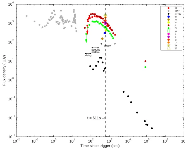
gath-ered from the literature and are compiled in Table2. Fig.1
displays the resulting light curves.
All magnitudes were then converted into the AB sys-tem, if required. The correction for the Galactic extinction was applied at the same time, using a value of E(B-V) = 0.024 (Schlafly & Finkbeiner 2011). The reddening due to the host galaxy is left as free parameter in fits to be
dis-cussed below. This leads to the corrections listed in Table1.
We then computed from the corrected magnitudes the flux density, using a zero point value of 23.926. The final flux
density light curves are presented in Fig.1.
3.2 Fermi data
GBM data for GRB 141221A were downloaded from the NASA/GSFC Fermi GBM Archive. The extraction of GBM data was done by using only the NaI detectors with the brightest signal in the 8keV – 1MeV band. In the case of GRB 141221A, these detectors were NaI 01 and NaI 02. We
used the taskRMFIT(v432)for data reduction, using the event
files (TTE) of each good detector.
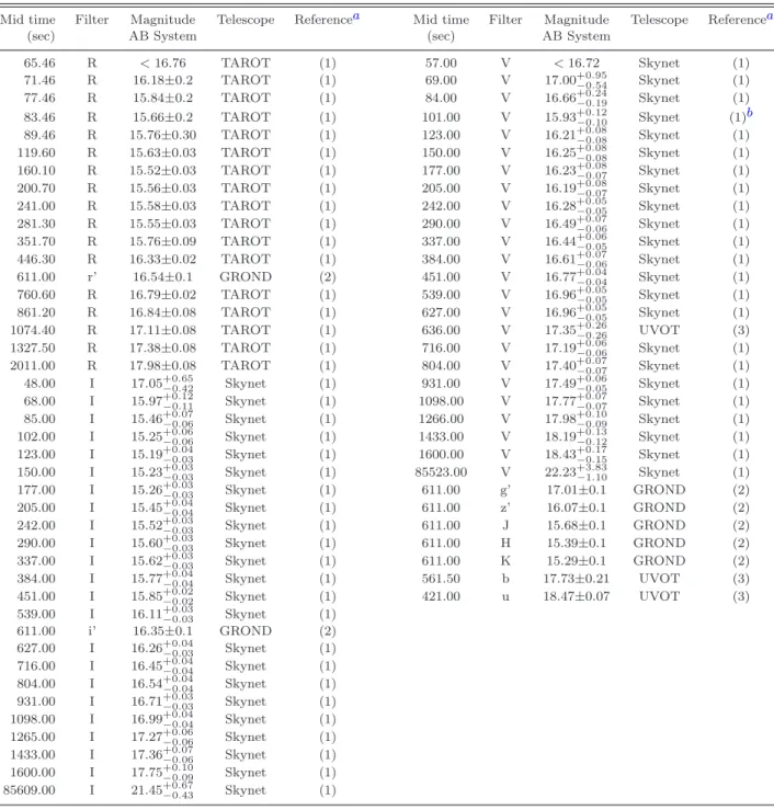
Table 2.Optical data converted into the AB System and corrected for Galactic extinction.
Mid time Filter Magnitude Telescope Referencea Mid time Filter Magnitude Telescope Referencea
(sec) AB System (sec) AB System
65.46 R <16.76 TAROT (1) 57.00 V <16.72 Skynet (1)
71.46 R 16.18±0.2 TAROT (1) 69.00 V 17.00+0.95
−0.54 Skynet (1)
77.46 R 15.84±0.2 TAROT (1) 84.00 V 16.66+0.24
−0.19 Skynet (1)
83.46 R 15.66±0.2 TAROT (1) 101.00 V 15.93+0.12
−0.10 Skynet (1)
b
89.46 R 15.76±0.30 TAROT (1) 123.00 V 16.21+0.08
−0.08 Skynet (1)
119.60 R 15.63±0.03 TAROT (1) 150.00 V 16.25+0.08
−0.08 Skynet (1)
160.10 R 15.52±0.03 TAROT (1) 177.00 V 16.23+0.08
−0.07 Skynet (1)
200.70 R 15.56±0.03 TAROT (1) 205.00 V 16.19+0.08
−0.07 Skynet (1)
241.00 R 15.58±0.03 TAROT (1) 242.00 V 16.28+0.05
−0.05 Skynet (1)
281.30 R 15.55±0.03 TAROT (1) 290.00 V 16.49+0.07
−0.06 Skynet (1)
351.70 R 15.76±0.09 TAROT (1) 337.00 V 16.44+0.06
−0.05 Skynet (1)
446.30 R 16.33±0.02 TAROT (1) 384.00 V 16.61+0.07
−0.06 Skynet (1)
611.00 r’ 16.54±0.1 GROND (2) 451.00 V 16.77+0.04
−0.04 Skynet (1)
760.60 R 16.79±0.02 TAROT (1) 539.00 V 16.96+0.05
−0.05 Skynet (1)
861.20 R 16.84±0.08 TAROT (1) 627.00 V 16.96+0.05
−0.05 Skynet (1)
1074.40 R 17.11±0.08 TAROT (1) 636.00 V 17.35+0.26
−0.26 UVOT (3)
1327.50 R 17.38±0.08 TAROT (1) 716.00 V 17.19+0.06
−0.06 Skynet (1)
2011.00 R 17.98±0.08 TAROT (1) 804.00 V 17.40+0.07
−0.07 Skynet (1)
48.00 I 17.05+0.65
−0.42 Skynet (1) 931.00 V 17.49
+0.06
−0.05 Skynet (1)
68.00 I 15.97+0.12
−0.11 Skynet (1) 1098.00 V 17.77
+0.07
−0.07 Skynet (1)
85.00 I 15.46+0.07
−0.06 Skynet (1) 1266.00 V 17.98
+0.10
−0.09 Skynet (1)
102.00 I 15.25+0.06
−0.06 Skynet (1) 1433.00 V 18.19
+0.13
−0.12 Skynet (1)
123.00 I 15.19+0.04
−0.03 Skynet (1) 1600.00 V 18.43
+0.17
−0.15 Skynet (1)
150.00 I 15.23+0.03
−0.03 Skynet (1) 85523.00 V 22.23
+3.83
−1.10 Skynet (1)
177.00 I 15.26+0.03
−0.03 Skynet (1) 611.00 g’ 17.01±0.1 GROND (2)
205.00 I 15.45+0.04
−0.04 Skynet (1) 611.00 z’ 16.07±0.1 GROND (2)
242.00 I 15.52+0.03
−0.03 Skynet (1) 611.00 J 15.68±0.1 GROND (2)
290.00 I 15.60+0.03
−0.03 Skynet (1) 611.00 H 15.39±0.1 GROND (2)
337.00 I 15.62+0.03
−0.03 Skynet (1) 611.00 K 15.29±0.1 GROND (2)
384.00 I 15.77+0.04
−0.04 Skynet (1) 561.50 b 17.73±0.21 UVOT (3)
451.00 I 15.85+0.02
−0.02 Skynet (1) 421.00 u 18.47±0.07 UVOT (3)
539.00 I 16.11+0.03
−0.03 Skynet (1)
611.00 i’ 16.35±0.1 GROND (2) 627.00 I 16.26+0.04
−0.03 Skynet (1)
716.00 I 16.45+0.04
−0.04 Skynet (1)
804.00 I 16.54+0.04
−0.04 Skynet (1)
931.00 I 16.71+0.03
−0.03 Skynet (1)
1098.00 I 16.99+0.04
−0.04 Skynet (1)
1265.00 I 17.27+0.06
−0.06 Skynet (1)
1433.00 I 17.36+0.07
−0.06 Skynet (1)
1600.00 I 17.75+0.10
−0.09 Skynet (1)
85609.00 I 21.45+0.67
−0.43 Skynet (1)
a References for the data: (1) this work, (2)Schweyer et al.(2014), (3)Marshall & Sonbas(2014) b This point exhibits an instrumental bias and has not been included in the analysis
3.3 X-Ray data
The data for GRB 141221A were downloaded from the
NASA/GSFCSwift Data Center and were processed using
HEASoft(v6.16) and the XRTDAS software version 0.13.1, with the latest calibration files available in June 2015. We
used the task xrtpipeline to create the clean event file
and to apply the latest calibration. We then performed a screening for bad pixels and piled-up data, using the meth-ods and corrections indicated in (Romano et al. 2006) and
(Vaughan et al. 2005). We found that the flare observed in
PC mode is piled-up during the intervalT0 + 138.2 s –T0
10−2 10−1 100 101 102 103 104 105 106 107 10−3
10−2 10−1 100 101 102 103 104
t = 611s →
rising pseudo plateau
decay
Time since trigger (sec)
Flux density (
µ
Jy)
R BAT x−ray b u v I V g r i z J H K
Figure 1.Flux density light curve of GRB 141221A. The vertical dashed line represents the epoch when the SED was extracted (see text for details).
4 DATA ANALYSIS 4.1 Prompt data
As already indicated, the prompt light curve has a duration
(T90) of about 23.8 seconds in Fermi-GBM and about 37s
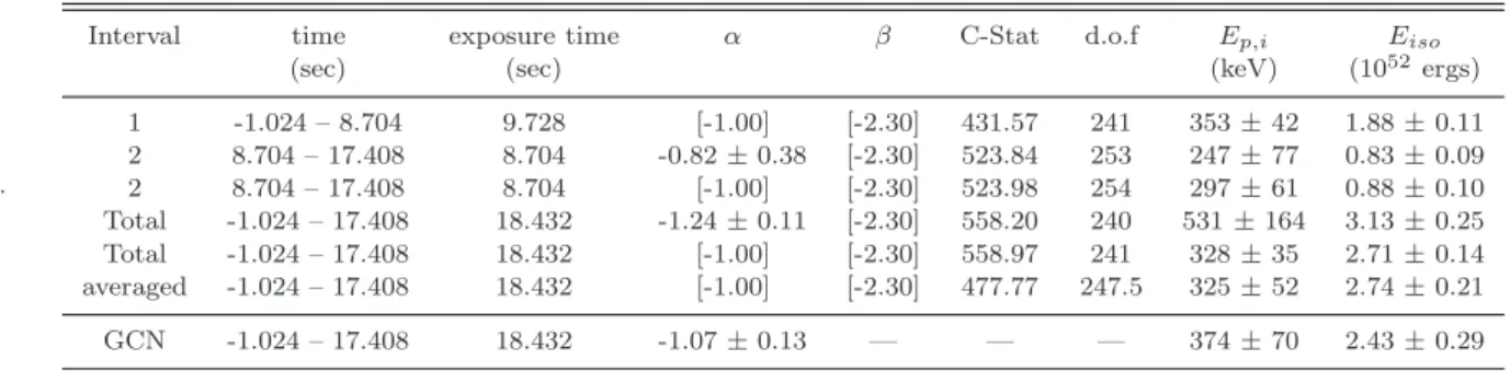
in Swift-BAT, and consists of two pulses. For the spectral analysis of prompt emission we used the Fermi/GBM instead ofSwift/BAT data because of the much larger energy band of the former instrument. We used Xspec version 12 (Arnaud 1996) to fit the spectrum with a Band model (Band et al. 1993). We first fit each pulse separately (named Intervals 1 and 2, respectively), and then fit the complete spectrum. We also took an average of the two pulse results. All the
results are displayed in Table3, together with a reminder of
the GCN result (Yu H.F. 2014). The low signal prevented us from fitting all the Band parameters separately, and in
all cases we had to fix theβparameter to a value of -2.3.
KnowingEpeak and the distance of this burst, we have
calculated Ep,i = 374±70 keV andEiso= 2.4×1052 erg.
We note that these values follow the Ep,i−Eiso relation
(Amati et al. 2009,2002), as can be seen in Fig.2.
4.2 Temporal decay
4.2.1 X-ray
The X-ray temporal analysis was already done for the ex-traction of the SED. The light curve presents a prominent flare, peaking at about 340 seconds. The remainder of the
1e+48 1e+49 1e+50 1e+51 1e+52 1e+53 1e+54
100
101
102
103
104
Eiso (ergs)
Ep,i (keV)
all GRBs GCN total avaraged
Figure 2.Our GRB compared to the whole sample of GRBs until June 2013. The solid line isEp,i= 110∗E0.57iso , while the dashed line is the 2 sigma standard deviation (Amati et al. 2009).
afterglow light curve is well fit by a simple power law, as can
be seen in Table4and Fig.1.
4.2.2 Optical
Table 3.Results of the prompt spectral fitting. Non-constrained parameters are fixed to the values indicated in square brackets
.
Interval time exposure time α β C-Stat d.o.f Ep,i Eiso
(sec) (sec) (keV) (1052ergs)
1 -1.024 – 8.704 9.728 [-1.00] [-2.30] 431.57 241 353±42 1.88±0.11 2 8.704 – 17.408 8.704 -0.82±0.38 [-2.30] 523.84 253 247±77 0.83±0.09 2 8.704 – 17.408 8.704 [-1.00] [-2.30] 523.98 254 297±61 0.88±0.10 Total -1.024 – 17.408 18.432 -1.24±0.11 [-2.30] 558.20 240 531±164 3.13±0.25 Total -1.024 – 17.408 18.432 [-1.00] [-2.30] 558.97 241 328±35 2.71±0.14 averaged -1.024 – 17.408 18.432 [-1.00] [-2.30] 477.77 247.5 325±52 2.74±0.21
GCN -1.024 – 17.408 18.432 -1.07±0.13 — — — 374±70 2.43±0.29
Table 4.Best fit temporal decay indices for the I, R, V and X-ray bands. Numbers in parentheses are not constrained by the fit. See text for details.
time filter model α1 α2 α3 tbreak tbreak,2 χ2ν d.o.f
(sec) (sec) (sec)
48 - 337 I broken power law −1.6±0.9 0.5±0.2 — 110±13 — 1.67 6 337 - 85609 I broken power law 1.0±0.2 1.6±0.4 — 918±160 — 1.53 9 281 - 2011 R 2 broken power law 1.6±0.4 0.4±3.2 1.3±0.9 540±514 906±696 1.36 1
69 - 205 V broken power law (−1.6) 0.1±1.2 — (109) — 0.10 1
205 - 85523 V broken power law 0.7±0.1 1.3±0.3 — 641±125 — 0.70 12
5800 - 191504 X-ray power law 1.4±0.2 — — — — 1.31 6
Table 5. Simple power law decay fit of the I, R, V bands. See text for details.
Filter α χ2
ν d.o.f I 1.12±0.10 3.83 11 V 0.91±0.10 2.57 14 R 1.04±0.22 10.6 6
We split the study in two parts, namely the rising and the decaying parts.
For the rise, we used a broken power law model. This gives us the end time of the fast rise and the start of the pseudo-plateau phase. In a few cases, the lack of data pre-vented an accurate measure, and we indicate these as
num-bers in parentheses in Table 4. This is the case for the R
band, which we attribute to an instrumental bias (see be-low).
For the decay, we first tried a simple power law model.
As one can see in Table 5, this model is strongly rejected
in all bands. We then inserted a break in the power laws,
obtaining good fits in the V and I bands (see Table4).
How-ever, this model, surprisingly, still does not fit the R band. In that band, we need a double broken power law in order to obtain a correct fit. At that point, the degrees of freedom are too low to ensure a correct measurement of the errors.
This double broken power law model mimics the stan-dard Swift X-ray light curve (i.e. a steep-flat-steep shape), but is not seen in the other bands. We explain this feature by the fact that these R band measurements come from the TAROT telescope, which was unfiltered to maximize its sen-sitivity. We have normalized the magnitudes to the Cousin R band assuming a template afterglow spectrum that does not contain any break. The TAROT CCD camera is sen-sitive from the I to the V bands (the B sensitivity is very
low). A spectral break that appears partly in the observa-tion window will not be accounted for. This can introduce an error in the reduced R magnitude that will depend on the position of the break. If the break is in the blue part of the spectrum, then the R magnitude will be underestimated, and vice-versa for the opposite case. The crossing of a spec-tral break would then translate into a steep-flat-steep shape in the light curve during the whole time of the crossing. This is not observed for the other bands (I and V) as standard filters have been used. The fits in the V and I bands (decay)
are presented in Fig.3.
4.3 Afterglow spectrum
We started by analyzing the XRT spectrum alone, indepen-dently of the optical data. This is because at high energy (above 2 keV), the spectrum is not influenced by the sur-rounding medium and the column density, and thus the X-ray spectrum allows us to derive the intrinsic power law in-dex. We extracted three spectra, one in WT mode and two in PC mode (during the flare, and after the flare), and fit these with a power-law model absorbed twice (one let free to vary at the distance of the burst, the second fixed to the galactic
value in the direction of the burst,NHgal= 2.27×10
20cm−2).
The data are consistent with no spectral variation, though we note that the error bars are large due to the low flux of the afterglow. The results of these fits are presented in Table 6. The lack of spectral variation is clearly confirmed by an analysis of the hardness ratio (using the hard and soft bands of 2.0-10.0 keV and 0.5-2.0 keV respectively) presented in Fig.4. While we see at the end of the flare a possible hard-ening of the spectrum, the error bars are still consistent with
no spectral variation at the 3σlevel.
Distribu-103 104
100
102
Flux density (
µ
Jy)
103 104 105
−100 −50 0 50 100
Time since trigger (sec)
Residuals
103 104
100
102
Flux density (
µ
Jy)
103 104 105
−100 −50 0 50 100
Time since trigger (sec)
Residuals
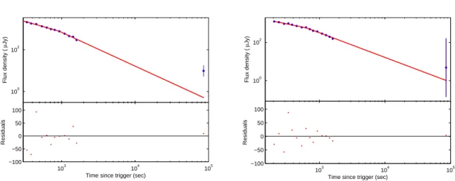
Figure 3.The best fit in the I (left) and V (right) bands with a power-law decay, starting from the end of the pseudo-plateau. The lower parts of each figure show the residuals of the fits.
Table 6.X-ray spectral analysis, independent of the optical mea-surements. See text for details.
Interval mode Nhost
H βx χ2ν d.o.f.
(sec) (1022cm−2)
60 - 90 WT 0.27+2.3
−0.27 0.7
+0.7
−0.5 1.02 6
100 - 1000 PC 0.9+0.5
−0.4 1.0
+0.4
−0.4 0.96 15
3000 - 11000 PC 0.5+0.6
−0.4 1.0
+0.4
−0.4 0.89 7
102 103 104 105 106
−0.4 −0.2 0 0.2 0.4 0.6 0.8 1 1.2
Time since trigger (sec)
Hardness Ratio(2.0−10.0keV/0.5−2.0keV)
Figure 4.Hardness ratio of the X-ray observation. We used the hard and soft bands of 2.0-10.0 keV and 0.5-2.0 keV respectively, only in PC mode.
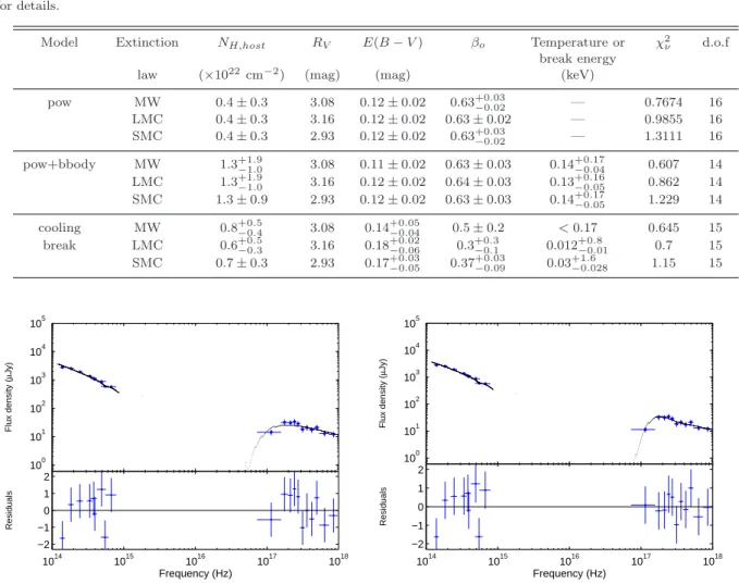
tion (SED), this time using all data available. We extracted the SED where the data were the most numerous, at about
611 s post burst (see Fig.1). This corresponds to the end of
the flare in X-ray and the decay phase of the optical band. In X-ray, we used the data taken between 350 and 619.7 sec-onds, and normalized them to the underlying afterglow flux. This last point is important: as there is no hint of flare in the optical light curve, it should not be linked to the X-ray flare. The non-variability of the hardness ratio makes us confident that this renormalization is enough to correct for the
pres-ence of the flare. All data (including the optical data) were then imported into XSPEC for the spectral fitting.
To model the SED, we consider single power law,
double power law and thermal components (see Table 7).
In all cases, we added foreground absorption by our own Galaxy (this absorption was fixed to the measured values of Kalberla et al. 2005, the optical extinction being corrected before the insertion into XSPEC), and by the distant host galaxy. We consider the three standard extinction laws, i.e., the Milky Way (MW), the Large Magellanic Cloud (LMC) and the Small Magellanic Cloud (SMC) ones. In all cases, the high energy power law index was allowed to vary freely only within the measured X-ray confidence interval. We first considered a simple power law extincted model. Even if the
fit quality seems good (see Table7), an analysis of the
resid-uals shows that this model does not fit the data correctly: it exhibits a lack of emission in the soft X-ray part of the SED
(see Fig.5). We then inserted a thermal component into the
model, and redid the analysis. This time, both the quality indicator of the fit and the residuals are in agreement with a good solution. We also tested the hypothesis of a cooling break, i.e., a broken power law with the two spectral indices
linked together by a difference ofβX =βo+ 0.5, which also
provides an acceptable fit.
As can be seen, the addition of the optical data strongly constrains the spectral index of the power law to a very low value. On the other hand, from this fit we cannot discrimi-nate between a Galactic or a Large Magellanic Cloud law of extinction. We present the best fit SED (assuming a power law model with an additional thermal component) in Fig. 5, using the LMC law, which is more common for GRBs compared to the MW law (Stratta et al. 2004).
5 DISCUSSION
5.1 The thermal component
We first consider the possibility that the thermal compo-nent seen in the SED is real. This would not be the first time such a component has been observed in the Swift era
(Starling et al. 2013; Sparre & Starling 2013). It has been
Table 7.Results of the spectral analysis of the SED.βois the power law index in case of a single power law. In case of a broken power law, this is the spectral index of the low energy segment, the high energy segment being linked to it by the relationβx=βo + 0.5. See text for details.
Model Extinction NH,host RV E(B−V) βo Temperature or χ2ν d.o.f break energy
law (×1022cm−2) (mag) (mag) (keV)
pow MW 0.4±0.3 3.08 0.12±0.02 0.63+0.03
−0.02 — 0.7674 16
LMC 0.4±0.3 3.16 0.12±0.02 0.63±0.02 — 0.9855 16 SMC 0.4±0.3 2.93 0.12±0.02 0.63+0.03
−0.02 — 1.3111 16
pow+bbody MW 1.3+1.9
−1.0 3.08 0.11±0.02 0.63±0.03 0.14
+0.17
−0.04 0.607 14
LMC 1.3+1.9
−1.0 3.16 0.12±0.02 0.64±0.03 0.13
+0.16
−0.05 0.862 14
SMC 1.3±0.9 2.93 0.12±0.02 0.63±0.03 0.14+0.17
−0.05 1.229 14
cooling MW 0.8+0.5
−0.4 3.08 0.14
+0.05
−0.04 0.5±0.2 <0.17 0.645 15
break LMC 0.6+0.5
−0.3 3.16 0.18
+0.02
−0.06 0.3
+0.3
−0.1 0.012
+0.8
−0.01 0.7 15
SMC 0.7±0.3 2.93 0.17+0.03
−0.05 0.37
+0.03
−0.09 0.03
+1.6
−0.028 1.15 15
100 101 102 103 104 105
Flux density (
µ
Jy)
1014 1015 1016 1017 1018 −2
−1 0 1 2
Residuals
Frequency (Hz)
100 101 102 103 104 105
Flux density (
µ
Jy)
1014 1015 1016 1017 1018 −2
−1 0 1 2
Residuals
Frequency (Hz)
Figure 5.The SED of GRB 141221A, fit with various models. On the left, a simple power law model. On the right, a simple power law plus a thermal component. In both cases, we use the LMC extinction law to fit the optical data. The bottom panels show the residuals for each model.
onto the surface of the progenitor or the emission of a hot cocoon protecting the jet during its travel into the progen-itor (Butler 2007). We note incidentally that this last ex-planation was also proposed to describe the early emission
of ultra-long GRBs (Gendre et al. 2013; Piro et al. 2014),
even if, as in this case, the burst does not belong to that class of events. As no supernova has been reported for GRB 141221A, we do favor the hypothesis of the hot cocoon.
If this component is really present, then the SED in-dicates that the optical and X-ray emissions are linked to-gether, and are thus due to the same emission mechanism. Indeed, at late times, all the temporal decay indices are com-patible, within errors. However, the SED is extracted before the final break of the I band, and thus this should also apply to earlier measurements. We do not see any evidence of a break in the X-ray light curve: this can be explained by the presence of the flare, which masks out the actual evolution of the afterglow. Moreover, the break times of the I and V magnitudes are compatible, within errors.
This light curve break is then achromatic, which is
con-sistent with a jet break (Rhoads 1997,1999). We obtain a
value of p = 1.28±0.06 which is extremely low. In
addi-tion, the jet break time is also extreme (about 750 s, while a
common pre-Swift value is on the order of daysGendre et al.
2006). This would lead to a jet opening angle of 1.3 degrees
(assuming the standard law ofSari & Piran 1999), and could
explain why in most cases no jet break is observed for Swift bursts: the break is looked for around a few hours (or days) after the trigger, and not at that earlier time.
In addition to this surprising value of the jet opening angle (that would put strong constraints on the SFR of mas-sive stars in the Universe), the only argument against this hypothesis is the R band behavior, that does not follow the V and I bands. In the previous section, we have explained this behavior by the fact that the break time was not iden-tical in all bands. If we suppose a constant break time, we cannot explain the R band behavior.
5.2 The rising and early decay of the afterglow
emissions are not linked to the same emission mechanism at the time of the SED (611 s). We can then assume that the various breaks we see are due to the passing through of a specific frequency into the observation bands, and that at a late time (¿ about 1000 s), the crossing of this frequency has ended and all the emission is due to the same emission mechanism.
The temporal break times in the I and V bands indicate that this specific frequency is decreasing with time, and, as already explained, the R band behavior is also compatible with that hypothesis. This leads us to exclude the passing through of the cooling frequency in a wind medium, as this frequency increases with time in such a case (Chevalier & Li 1999; Panaitescu & Kumar 2000). If we still assume the wind medium, the only remaining option is the injection
frequency,νm. However, the spectral index before the
cross-ing (0.3+0.3
−0.1) would lead to a value ofplower than 1, which is
not physical. We thus can conclude that these breaks cannot be explained in the case of the wind medium.
The situation is different in case of the ISM. There, we can logically assume that the last two breaks are linked to the injection and cooling breaks, respectively. The injection
and cooling frequencies vary ast−1.5andt−0.5respectively.
Taking into account the errors on the break times, all break measurements are compatible with this explanation. After the cooling break, the spectral and the temporal decay
in-dices are all compatible with a value of p∼2.5±0.3. The
early spectral index (before the cooling break, as measured
in the optical) should beβ= 0.7±0.2, compatible with the
measurement (0.3+0.3
−0.04).
In this scenario, the end of the ”pseudo-plateau” phase is the injection break, i.e., the peak of the afterglow. Again, the variation of the break time between the V and I bands is consistent with this hypothesis. Then, however, the tem-poral decay indices of the ”pseudo-plateau” should become negative. This does not agree with the model. We explain it by the contribution of a small reverse shock that masks the peak of the emission. We can then, assuming the surround-ing medium density to be equal to one, and the efficiency of the fireball in radiating its energy to be 30 %, compute the microphysical parameters of the fireball, using the work of Panaitescu & Kumar (2000). Doing so, we obtain the
fire-ball total energy (E= 8×1052erg), the magnetic parameter
(ǫB= 5×10⁻²), and the electron parameter (ǫe= 3×10⁻³).
These numbers are relatively normal (see e.g.Gendre et al.
2008), albeitǫBis slightly higher than usually seen. We thus
have a complete description of the afterglow of this burst. We note, however, the total absence of a stellar wind in that model.
Chevalier et al. (2004) have pointed out the complex surrounding medium of a GRB. However, assuming that the progenitor for all long GRBs is a stellar object (Woosley 1993), we still should observe a small portion of the light curve where a wind environment should be present. Here, from about 200 seconds after the trigger to the end of the observations, the medium is compatible with an ISM only. It is a well-known fact that most of Swift bursts are compatible with an ISM, but a degeneracy prevents excluding the wind medium hypothesis (Chevalier et al. 2004). Here, we have the proof that the wind medium is rejected from nearly the start of the afterglow, leaving only extreme constraints on the stellar physics in order to suppress the stellar wind from
the progenitor. It is beyond the scope of this paper to in-troduce such a stellar model, however GRBs are known to
have weak stellar winds (e.g.Gendre et al. 2004,2013), and
thus such a model would be very useful. We conclude this
section by noting that the intrinsic values ofEB−V and NH
are low, and thus again are compatible with a low density around this GRB.
5.3 Absorption and Extinction
From our analysis, it turns out that we obtain a bet-ter solution using an LMC extinction law, because the
observed GROND g-band is best fit by 2175 ˚A
absorp-tion feature present in LMC (and MW). We note that best-fit solutions with LMC or MW dust have already
been observed (e.g.,Kann et al. 2006; Kr¨uhler et al. 2008;
Kann et al. 2010), even if other models may be more appro-priate (Stratta et al. 2004). However, given that these data were obtained from the preliminary photometry quoted in Schweyer et al.(2014), and that they do not have apprecia-ble influence on the fitted parameter values, we prefer to leave this argument for a future work when better data will be available.
All the spectral models we tried favor a slightly dusty
environment withE(B−V)∼0.1−0.2 (see Table7). These
values are not unusual (Kann et al. 2010; Greiner et al.
2011;Zafar et al. 2011), most of all at the distance of GRB
141221A (Kann et al. 2006; Covino et al. 2013). The
ob-served NH,host is also in agreement with those found for
other bright bursts, especially when compared with the
best-fit optical extinction in the redshift interval 1< z <2 (e.g.
Watson et al. 2013; Covino et al. 2013). Like many other
bursts, the metals-to-dust ratio (NH,host/AV) is in the range
1−3×1022cm−2mags−1 (Zafar et al. 2011;Kr¨uhler et al.
2011;Covino et al. 2013).
We finally note that the extinction is not enough to set
the optical to X-ray spectral index below the valueβO−X=
0.5 (see Table7), and thus we cannot consider GRB 141221A
as a dark GRB (Jakobsson et al. 2004;Rossi et al. 2012).
6 CONCLUSIONS
We have analyzed the observations of GRB 141221A made in optical and high energy bands by various instruments, including TAROT and Skynet. In X-ray bands, the burst is very similar to all the previous ones observed, with a late flare. In optical bands, however, the light curve shows a rising part, a pseudo-plateau phase, and various tempo-ral breaks. We explain these breaks as due to the passing through of several specific frequencies into the optical bands. We need a minimal contribution by a reverse shock to com-pletely explain both the optical and X-ray light curves and spectra.
Clearly, both solutions are challenging for GRB models. In the former case, all the data point toward an absence of stellar wind during the whole phenomenon, which is in contradiction with current models. In the latter case, the microphysics parameters obtained by the model are very unusual, and in some cases not really taken into account by the model. GRB 141221A should thus be added to the short list of very constraining bursts against which each new model should be tested.
ACKNOWLEDGMENTS
We thank the anonymous referee for her/his helpful com-ments that helped to improve this paper. O.Bardho is sup-ported by the Erasmus Mundus Joint Doctorate Program by Grant Number 2012-1710 from the EACEA of the Eu-ropean Commission. This research has made use of the XRT Data Analysis Software (XRTDAS) developed under the responsibility of the ASI Science Data Center (ASDC), Italy. BG acknowledges financial support of NASA through the NASA Award NNX13AD28A and the NASA Award NNX15AP95A. AR, and EP acknowledge support from PRIN-INAF 2012/13. This work is under the auspice of the FIGARONet collaborative network, supported by the Agence Nationale de la Recherche, program ANR-14-CE33.
REFERENCES
Amati, L., Frontera, F., Tavani, M., 2002, A&A 390, 81 Amati, L., Frontera, F., Guidorzi, C., 2009, A&A 508, 173 Arnaud, K.A., 1996, Astronomical Data Analysis Software and
Systems V, eds. Jacoby G. and Barnes J., p17, ASP Conf. Series volume 101
Band, D., Matteson, J., Ford, L., et al., 1993, ApJ 413, 281 Beardmore, A.P., Evans, P.A., Goad, M.R., et al., 2014, GCN
#17211
Bo¨er, M., Klotz, A., Atteia, J.-L., et al., 2003, The Messenger 113, 45
Butler, N.R., 2007, ApJ 656, 1001
Chevalier, R.A., & Li, Z.Y., 1999, ApJ 520, 29
Chevalier, R.A., Li, Z.Y., & Fransson, C., 2004, ApJ 606, 369 Covino, S., Melandri, A., Salvaterra, R., Campana, S., Vergani,
S. D., et al., 2013, MNRAS 432, 1231
Gehrels, N., Chincarini, G., Giommi, P., et al., 2004, ApJ 611, 1005
Gendre, B., Piro, L., & De Pasquale, M., 2004, A&A, 424, L27 Gendre, B., Corsi, A., & Piro, L., 2006, A&A 455, 803 Gendre, B., Galli, A., & Bo¨er, M., 2008, ApJ 683, 620 Gendre, B., Atteia, J. L., Bo¨er, M., et al., 2012, ApJ 748, 59 Gendre, B., Stratta, G., Atteia, J. L., et al., 2013, ApJ 766, 30 Greiner, J., Bornemann, W., Clemens, Ch., et al., 2008, PAASP
120, 405
Greiner, J., Kr¨uhler, T., Klose, S., Afonso, P., Clemens, C., et al., 2011, A&A 526, 30
Jakobsson, P., Hjorth, J., Fynbo, J.P.U., Watson, D., Pedersen, K., et al., 2004, ApJ, 617, L21
Kalberla et al. 2005, A&A, 440, 775
Kann, D.A., Klose, S., Zeh, A., 2006, ApJ 641, 993,
Kann, D.A., Klose, S., Zhang, B., Malesani, D., Nakar, E., et al., 2010, ApJ 720, 1513
Klotz, A., Vachier, F., Bo¨er, M., et al., 2008, AN 329, 275 Klotz, A., Turpin, D., Bo¨er, M., et al., 2014, GCN #17227 Kr¨uhler, T. K¨upc¨u Yolda¸s, A., Greiner, J. Clemens, C. McBreen,
S., et al., 2008, ApJ 685, 376
Kr¨uhler, T., Greiner, J., Schady, P., Savaglio, S., Afonso, P.M.J., et al., 2011, A&A 534, 108
Kr¨uhler, T., Malesani, D., Milvang-Jensen, B., Fynbo, J.P.U., Hjorth, J., et al., 2012, ApJ 758, 46
Kumar, P. & Zhang, B., 2015, Physics Reports 561, 1 Marshall, F.E. & Sonbas, E., 2014, GCN #17219
Maselli, A., Melandri, A., Sbarufatti, B., et al., 2014, GCN #17214
M´esz´aros, P, & Rees, M.J., 1997, ApJ, 476, 232 P. Meszaros, 2006, RPPh 69, 2259
Panaitescu, A., M´esz´aros, P., & Rees, M.J., 1998, ApJ, 503, 314 Panaitescu, A., & Kumar, P., 2000, ApJ 543, 66
Pei, Y.C., 1992, ApJ 395, 130
Perley, A.D., Cao, Y., Cenko, S.B., et al., 2014, GCN #17228 Piro, L., Troja, E., Gendre, B., et al., 2014, ApJ 790, 15 Racusin, J.L., Liang, E.W., Burrows, D.N., 2009, ApJ 698, 43 Rees, M.J., & M´esz´aros, P., 1992, MNRAS, 258, 41
Reichart, D., Nysewander, M., Moran, J, et al., 2005, Nuovo Ci-mento C, 28, 767
Rhoads, J.E., 1997, ApJ 487, L1 Rhoads, J.E., 1999, ApJ 525, 737
Romano, P., Campana, S., Chincarini, G., et al., 2006, A&A 456, 917
Rossi, A., Klose, S., Ferrero, P., Greiner, J., Arnold, L. A., et al., 2012, A&A 545, 77
Sari, R., and Tsvi, P., 1999, ApJ 520, 641
Schlafly, E.F. & Finkbeiner D.P., 2011, ApJ 737, 103
Schweyer, T., Wiseman, P., Schady, P., et al., 2014, GCN #17212 Sonbas, E., Cummings, J. R., D’Elia, V., et al., 2014, GCN
#17206
Sparre, M., & Starling, R.L.C., 2013, MNRAS 427, 2965 Starling, R.L.C., Page, K.L., Pe’er, A., et al., 2013, MNRAS 427,
2950
Stratta, G., Fiore, F., Antonelli, A., et al., 2004, ApJ, 608, 846 Trotter, A., Haislip, J., Reichart, D., et al., 2014, GCN #17210 Trotter, A., Haislip, J., Reichart, D., et al., 2014, GCN #17221 Ukwatta, T.N., Barthelmy, S.D., Baumgartner, W.H., et al., 2014,
GCN #17213
Vaughan, S., Goad, M.R., Beardmore, A.P., et al., 2005, ApJ 638, 920
Watson, D., Zafar, T., Andersen, A.C., Fynbo, J.P.U., Gorosabel, J., et al., 2013,ApJ 768, 23
Woosley, S.E., 1993, ApJ 405, 273 Yu H.F., 2014, GCN #17216