IET Communications
Research Article
Location-based coverage and capacity
analysis of a two tier HetNet
ISSN 1751-8628 Received on 19th October 2016 Revised 6th December 2016 Accepted on 8th December 2016 E-First on 11th April 2017 doi: 10.1049/iet-com.2016.1244 www.ietdl.org
Muhammad Mussawer Pervez
1, Ziaul Haq Abbas
1, Fazal Muhammad
1, Lei Jiao
21Faculty of Electrical Engineering, Ghulam Ishaq Khan Institute of Engineering Sciences and Technology, Topi, Swabi 23640, Khyber
Pakhtunkhwa, Pakistan
2Department of Information and Communication Technology, University of Agder (UiA), N-4879 Grimstad, Norway
E-mail: [email protected]
Abstract: Stochastic geometry tool is an accurate and tractable approach to analyse the performance characteristics of heterogeneous networks (HetNets) with unplanned deployment of base stations (BSs). In this study, the authors analyse the downlink coverage and capacity by taking into account the separation between the macro BS (MBS) and small BSs (SBSs) in a HetNet. MBSs, SBSs, and users are spatially distributed as independent Poisson point processes. The whole space is divided into inner and outer subspaces around the MBSs and a typical user is assumed to be in outer subspace. Analysis on the typical user in the outer subspace incorporates the effect of distance of SBSs from MBS. They derive the expressions for the coverage probability of an outer subspace typical user from SBS and MBS. They also derive the expressions for rate coverage of an outer subspace typical user from SBS and MBS. These metrics are analysed with varying inner subspace radius to incorporate the effect of BSs separation. Simulation results show that SBSs away from MBS in the coverage region of MBS provide good performance to their associated users in terms of coverage probability and rate coverage.
1 Introduction
An exponential growth in the volume of wireless traffic has been caused due to ubiquity of wireless devices and data hungry applications. This growth requires efficient increase in data rate density and peak data rate [1–3]. A promising solution to handle this issue is to increase spatial reuse of available resources through infrastructure densification. Small base stations (SBSs) are, therefore, deployed into existing infrastructure. This results in heterogeneous networks (HetNets) [4].
A HetNet comprises of different classes (tiers) of BSs. Each tier BSs differ in terms of transmit power, load, spatial density etc. When the SBSs are deployed within macro BS (MBS) coverage region, the spectrum efficiency is improved due to the sharing of radio resources [5, 6]. In [7], it is observed that user experience is improved when SBSs are deployed in the network even without using interference mitigation techniques. By using interference mitigation technique and range expansion for small cells, more users connect to the SBSs and overall user experience is further improved. Similarly, the deployment of femtocells in the indoor and picocells in the outdoor in addition to the conventional macro cells is a promising solution to increase the cellular network capacity in a cost efficient way [8]. Furthermore, HetNets result in improved performance for blind zone and cell edge users.
Since the coverage areas of SBSs and MBSs are overlapped in HetNets, high transmit power difference of MBS and SBS causes the coverage area of SBSs to be narrow in maximum received power association strategy [9, 10]. Therefore, the location of SBSs in the vicinity of an MBS is a key parameter that can alter the performance characteristics of SBSs and the overall network. It has been observed in [11] that choosing a large distance between MBS and SBS improves the performance of the network. In [12], it is observed that improvement in network performance is more when small cells are deployed at the edge of macro cell. Therefore, in performance of HetNets, location of SBSs plays a major role. The goal of this paper is to characterise the performance metrics such as coverage and data rate of SBSs based on their location in a two tier HetNet (comprising of an SBS tier and an MBS tier).
Coverage probability and rate coverage are two essential performance metrics that characterise the performance of a HetNet.
The BSs deployment strategies play a key role in evaluating these performance metrics. This is due to the fact that signal-to-interference plus noise ratio (SINR) statistics depends on location of BSs in the network and SINR is used to obtain these performance metrics. Therefore, in the literature several approaches have been proposed based on BSs location to analyse the coverage and rate of a cellular network [13–20].
A simple approach to model and analyse cellular networks is Wyner model [13–15] which provides analytical tractability by assuming unit channel gain from the serving BS and equal channel gain from all interferers. However, due to deterministic SINR, this model turns to be highly inaccurate for computing coverage probability in HetNets where different tiers’ BSs provide service to the users. Another approach is conventional hexagonal grid model which provides tractable SINR analysis for a fixed user only [16, 17]. In brief, this idealised and widely accepted model is inaccurate and intractable for HetNets. Spatial stochastic model [18–21] is another approach which is less accepted for planned scenarios but more realistic model for the networks with randomly deployed BSs. Stochastic geometry is therefore used to capture the randomness in the deployed BSs and gives accurate results for performance like coverage and rate. In [22], it is shown that using stochastic geometry, the SINR analysis of single tier, i.e. conventional macrocell network, is as accurate as a hexagonal grid model. This baseline model is further extended to general K-tier HetNet model in [23–25]. The coverage and rate analysis for a typical user based on its location in the network has not been investigated in their work.
In this paper, we consider a HetNet comprising of two tiers, i.e. MBSs tier and SBSs tier. We use stochastic geometry tool to study the coverage of SBSs while taking the separation of SBSs and MBS into account. The distributions of MBSs, SBSs, and users follow independent Poisson point processes (PPPs). Users adopt the maximum received power association scheme to connect with a BS of a particular tier. Rayleigh fading channels are assumed for all links [26]. To study the effect of SBSs and MBSs separation on coverage probability and rate coverage, each MBS coverage region is divided into inner subspace and outer subspace. Some SBSs belong to inner subspace and remaining belong to outer subspace.
A typical user is assumed to be in outer subspace and hence can associate to SBS or MBS depending on association strategy.
The major contributions of this paper are described as follows: i. The coverage probabilities of a typical user from SBS and
MBS are analysed considering the separation between SBSs and MBS in the network. In addition, the total coverage probability of a typical user is also analysed.
ii. Expressions for rate coverage of a typical user are derived while assuming that the typical user is in outer subspace. Rate coverage from SBS and total rate coverage are then inspected. The rest of this paper is organised as follows. Section 2 describes network model. Mathematical preliminaries are discussed in Section 3. In Sections 4 and 5, the expressions for coverage probability and rate coverage are derived, respectively. Results and discussion are given in Section 6. Section 7 concludes this paper.
2 Network model
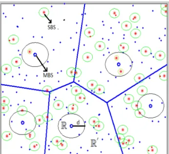
Our two tier is shown in Fig. 1. MBSs are randomly deployed in the plane using homogeneous PPP, Ψ1, with density λ1. SBSs and
users are also deployed using homogeneous PPPs, Ψ2 and Ψu, with
densities λ2 and λu, respectively. The dots, stars, and small circles in Fig. 1 represent users, SBSs, and MBSs, respectively. MBSs and SBSs have the transmit power Ptm and Pts, path loss exponents α1
and α2, and SINR thresholds τ1 and τ2, respectively. The whole
space is divided into two subspaces around the MBSs, i.e. inner subspace ℝ having radius d and outer subspace ℝ′. Rayleigh fading is assumed for all links and its impact is denoted by random variable h( . ) that follows independent and identical exponential distribution with unit mean, i.e. h ∼ exp(1).
A typical user, Tu, is assumed to be at origin in ℝ′ and the SINR analysis is carried out for this user. We also assume full buffer model, i.e. each BS in the network has data for transmission to its associated user and there is no unloaded BS. Furthermore, we use stochastic geometry tool to derive expressions for SINR and rate coverage. Table 1 shows the set of notations used in this paper.
3 Mathematical preliminaries
This section presents the mathematical preliminaries that will be utilised in the next section to model the performance metrics, i.e. coverage probability and rate coverage. The discussion begins with user association and SINR analysis which is followed by the statistical distance to serving BS. Per-tier association probability, load distribution of serving BS, and rate are also discussed subsequently.
3.1 User association and SINR analysis
On the basis of the maximum received power association scheme, a typical user associates to particular tier BS from which it receives maximum power. Mathematically, the location of serving BS, j, is written as
j = arg max
k ∈ m, sPtk| | xk| |
−αk,
(1) where xk is the distance of a typical user from the kth-tier serving
BS. If a typical user uses the above association scheme, its SINR expression can be obtained as given below.
If a typical user connects with an SBS located at x, the SINR received at the typical user can be written as
SINRs(x) =Ptshxx −α2
ICs+ σ2 , ∀x > 0, (2)
where hx is the fading coefficient of the desired link and σ2 is the
background noise power. ICs is the cumulative interference at the
typical user which is given as
ICs = I Cm+ ICs′ =
∑
y ∈ Ψ1Ptmhyy −α1 +∑
z ∈ Ψ2∖xPtshzz −α2 . (3)Here, ICm is the cumulative interference of MBSs and ICs′ is the cumulative interference of SBSs except the serving SBS. ∑y∈Ψ1Ptmhyy
−α1 represents interference from all MBSs distributed
as Ψ1. Since the serving BS belongs to SBSs’ tier represented by Ψ2; therefore, ∑z∈Ψ2∖xPtshzz
−α2 shows the interference from all
SBSs that belong to Ψ2 except the serving SBS located at x.
If a typical user connects with MBS located at x, the SINR received at the typical user can be written as
SINRm(x) = Ptmhxx
−α1
ICm+ σ2 , ∀x > d, (4)
Fig. 1 Illustration of network model. Circles around MBSs show inner subspaces, small circles around SBSs show coverage region of SBSs, and dots represent users
Table 1 Notations summary
Parameter Description
Ψ1, Ψ2, Ψu PPPs of the MBSs, SBSs, and users, respectively
λ1, λ2, λu spatial densities of MBSs, SBSs, and users,
respectively
σ2 noise power
Ptm, Pts transmission power of the serving MBSs and SBSs,
respectively
α1, α2 path loss exponent of MBSs and SBSs, respectively
τ1, τ2 SINR threshold of MBSs and SBSs, respectively 𝒜m′, 𝒜s′ per-tier association probability
ℝ, ℝ′ inner subspace and outer subspace, respectively X1, X2 statistical distances of the serving MBS and SBSs from
the typical user, respectively
h( . ) fading coefficients of the desired and interfering links 𝒞m′ ,𝒞s′ coverage probability of a typical user in the outer
subspace from MBS and SBS, respectively ℛcs ,ℛcm rate coverage of SBS and MBS, respectively
where ICm is the cumulative interference at the typical user which is given as ICm= I Cm′+ ICs =
∑
y ∈ Ψ1∖x Ptmhyy−α1+∑
z ∈ Ψ2 Ptshzz−α2. (5)Here, ICm′ is the cumulative interference of MBSs except the serving MBS and ICs is the cumulative interference of SBSs. These expressions are used to find the coverage probability of a typical user from SBS and MBS.
3.2 Statistical distance to serving BS
Since BSs are deployed as a PPP, the serving BS distance from a typical user is a random variable which is described by its probability density function (PDF). Denoting Xk as the distance between a typical user and its serving kth-tier BS, the distance distribution fXk|Tu ∈ℝ′(x) can be obtained as
fXk|Tu ∈ℝ′(x) = fXk(x)
P[Tu∈ ℝ′] . (6)
Using null probability of PPP [27], we can write
fXk(x) = 2πλkxe−λkπx
2
. (7)
The probability that a typical user is in ℝ′ is [28]
P[Tu∈ ℝ′] = e−λ1πd2. (8)
Now substituting (7) and (8) into (6), we get
fXk|Tu ∈ℝ′(x) =2πλkxe
−λkπx2
e−λkπd2 .
(9)
3.3 Per-tier association probability
A typical user in the network can associate to either tier with some probability. The probability that a typical user is associated with MBS's tier is
𝒜m′= λ1exp −π λ1+ λ2(Pts)2/αd2
λ1+ λ2(Pts)2/α
. (10)
If a typical user is associated with SBS's tier, the probability is given as
𝒜s′= λ2
λ2+ λ1(Ptm)2/α
. (11)
Proof: See Appendix 1.□
The probabilities, 𝒜m′ and 𝒜s′, are used to find the average number of users per BS of each tier.
3.4 Load distribution of serving BS
In our proposed model, the association region is considered as a Poisson–Voronoi (PV) tessellation. Hence, following the maximum received power association scheme, the coverage region of a k th-tier randomly distributed PV BS at x, S, is written as:
Sxk(Ψ) = y ∈ ℝ2: ∥ y − x k∥ ≤ Ptk Pti 1/αk ∥ y − xi∥1/α ^ k , ∀xk∈ Ψ, xi∈ Ψ, xk≠ xi,
where xi denotes the distance between the typical user and the serving BS. The random PV tessellation is obtained by the compendium of Sxk.
As BSs’ tiers are randomly distributed according to PPP, the average coverage area of the kth-tier BS is 𝒜k/λk. The k
th-tier-associated BS area is estimated as S 𝒜k/λk [29].
As no standard probability distribution function (PDF) exists for the Voronoi cell size, therefore, in a D-dimensional space, PDF for the PV area, s, can be written as [30]
fD(s) = (3D + 1)/2Γ (3D + 1)/2(3D+ 1)/2 𝒜λk ks (3D− 1)/2 exp − 3D + 12 𝒜λk ks , (12)
where Γ(t) = ∫0∞exp( − z)zt− 1dz denotes the standard gamma
function. Similarly, the PDF for the PV area of a kth-tier BS, Sk, in the 2D-plane is deduced from (12) as
fSk(s) = (7/2)Γ(7/2)7/2 𝒜λk ks
5/2
exp − 72 𝒜λkk s . (13)
Using (13), the probability mass function of the number of users associated to kth-tier BS is given as [29]
P[Nk= nk+ 1] = 3.5 3.5 nk! Γ(nΓ(3.5)k+ 4.5) λu𝒜k λk 3.5 +λuλ𝒜k k −(nk + 4.5) . (14)
Here, Nk denotes the typical user plus other associated users. Using (14), the load distribution of the serving MBS and SBS in ℝ′ can be written, respectively, as P[Nm= nm+ 1] = 3.5n 3.5 m! Γ(nm+ 4.5) Γ(3.5) λu𝒜λ1m′ 3.5 +λu𝒜m′ λ1 −(nm + 4.5) , (15) and P[Ns= ns+ 1] = 3.5n3.5 s! Γ(ns+ 4.5) Γ(3.5) λu𝒜s′ λ2 3.5 +λuλ𝒜s′ 2 −(ns + 4.5) . (16) 3.5 Rate
Under the assumption of saturated resource allocation scheme, each user receives a rate proportional to the spectral efficiency of its link. Therefore, the rate of a user associated with SBS and MBS, ℛs and ℛm, respectively, can be written as
ℛs= BWN
s log21 + SINRs(x) , (17)
ℛm= BWN
m log21 + SINRm(x) . (18)
Here, BW is the available bandwidth. These expressions are utilised in Section 5 to find the rate coverage of a typical user from MBS and SBS.
Hence, we have obtained the expressions for SINR, statistical distance to serving BS, per-tier association probability, load distribution of serving BS, and rate. These expressions are useful to find the performance metrics, i.e. coverage probability and rate coverage.
4 Coverage probability
The coverage probability, which is also called SINR coverage, is defined as the probability that the instantaneous SINR of a typical user from a serving BS is greater than a target SINR. This is equivalently the complementary cumulative distribution function of SINR. When a typical user is associated with MBS located at x, the coverage probability can be written as
𝒞m′(τ1) = Ex(P[SINRm(x) > τ1]), (19)
where τ1 is the target SINR of MBS. 𝒞m′ represents the coverage probability averaged over the coverage of MBS. This metric shows the average fraction of area that is under coverage at any time. Ex
denotes the expectation with respect to x. The following result can be obtained from (19): 𝒞m′(τ1) = 𝒦m
∫
d ∞ x exp −τ1 SNR − π(λ1Z′m+ λ2Z′′m+ λ1x2) dx . (20) Here, 𝒦m≡ 2πλ1/e−λ1πd2, Z m ′ ≡ Z(QPtm, α1, x α1 ), Zm′′ ≡ Z(QPts, α2, Pts)xα1, Q ≡ xα1τ/Ptm, and Z(a, b, c) ≡ (a)2/b∫ (c/a)(2/b)∞ (dm/(1 + mb/2)) .Similarly, the SINR
coverage of a typical user when it is associated with SBS can be written as
𝒞s′(τ2) = Ex(P[SINRs(x) > τ2]), (21)
which gives the following result: 𝒞s′(τ2) = 𝒦s
∫
0 ∞
x exp −τ2
SNR − π(λ2Z′s+ λ1Z′′s+ λ2x2) dx . (22)
Here, τ2 is the target SINR of SBS, 𝒦s≡ 2πλ2/e −λ1πd2 , Zs′ ≡ Z(Q′Pts, α2, x α2 ), and Zs′′ ≡ Z(Q′Ptm, α1, d α2 ).
Proof: See Appendix 2.□
5 Rate coverage
The rate coverage is defined as the probability that the rate of a typical user from a serving BS is greater than a target rate. When a typical user associates to SBS, its rate coverage [It is worth mentioning that ℛs and ℛm in (17) and (18) represent the rate of a typical user from SBS and MBS, respectively; while ℛcs and ℛcm
in (24) and (25) represent the rate coverage of a typical user from SBS and MBS, respectively.], ℛcs, can be written as
ℛcs = P[ℛs> η], (23) where η is the target rate. Equation (23) gives the following result:
ℛcs =
∑
ns≥ 0 3.53.5 ns! Γ(nΓ(3.5)s+ 4.5) λu𝒜s′ λ2 3.5 + λu𝒜s′ λ2 −(ns + 4.5) 𝒞s′ (2η(ns + 1)/BW− 1) . (24)Similarly, if a typical user associates to MBS, its rate coverage, ℛcm, can be written as ℛcm =
∑
nm≥ 0 3.53.5 nm! Γ(nΓ(3.5)m+ 4.5) λu𝒜λ2m′ 3.5 +λu𝒜λm′ 2 −(nm + 4.5) 𝒞m′(2η(nm + 1)/BW− 1) . (25)Proof: See Appendix 3.□
6 Results and discussion
In this section, we present the numerical results obtained for coverage probability of a typical user from SBS and MBS in the outer subspace while considering users’ separation from MBS. The total coverage probability in the outer subspace is also analysed. We also present the results obtained for rate coverage from SBS and the total rate coverage in the same subspace. For the validation of our analytical results, simulation results for coverage probability and rate coverage are also presented. We take Ptm= 50 dBm,
Pts= 30 dBm, and λ1= 1 MBS/km2 for our calculations. We also
assume equal SINR thresholds and path loss exponents, i.e.
τ1= τ2= τ and α1= α2= α, respectively.
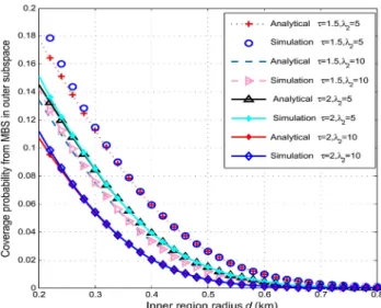
Fig. 2 shows the coverage probability of an outer subspace typical user from MBS. The coverage probability decreases with increase in radius of ℝ. This is due to the fact that increase in radius of the inner subspace causes a typical user to be at higher distance from MBS. This results in poor coverage probability from MBS. It is also observed that a typical user experiences smaller coverage probability at higher SINR threshold and SBSs density. When SBSs density increases, the number of SBSs in the outer region increases and hence the outer region users are more likely to obtain coverage from these SBSs. Furthermore, the analytical results are in close approximation with the simulation results. A slight difference in both results comes due to the fact that we make assumptions of Rayleigh fading and independency of PPPs to obtain analytical expressions.
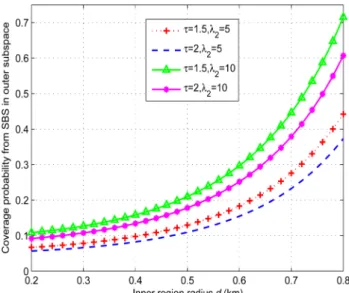
Fig. 3 illustrates the coverage probability of a typical user from SBS in ℝ′. With a larger radius of ℝ, the coverage probability is improved. The larger radius causes the outer region typical user to be at a greater distance from MBS. Thus, SBSs in that region
provide more coverage to their associated users due to smaller effect of MBS interference. Furthermore, the coverage probability is more for lower value of τ and higher value of λ2. This is because the users are more likely to obtain coverage from the associated BS at low SINR threshold and high BS density.
Total coverage probability, 𝒞t′, of a typical user is plotted in Fig. 4 using the following equation:
𝒞t′= 𝒞m′𝒜m′+ 𝒞s′𝒜s′.
A slight decrease is first observed with increase in radius of ℝ. This decrease in the coverage probability of a typical user from MBS is more than the increase in coverage probability from SBS. Afterwards, the total coverage probability increases due to more increase in coverage probability of a typical user from SBS. Thus, the users that are away from MBS in the coverage region of MBS have good coverage due to the effective utilisation of SBSs.
Fig. 5 illustrates the rate coverage of a typical user from SBS in ℝ′. Simulation results are also presented to show the validation of analytical results.
Since SBSs are deployed in the network to enhance the capacity, therefore, users that are associated to SBSs achieve better rate. This rate decreases with increase in the rate threshold as compared in Fig. 5. The rate coverage is improved as the typical user is assumed away from MBS by increasing the radius of ℝ. This is due to the fact that an SBS away from MBS has a higher probability of providing a pre-defined rate to its associated users.
In Fig. 6, the total rate coverage, ℛct, of a typical user is depicted by taking into account the distance from MBS. Total rate coverage can be obtained as
ℛct = ℛcm𝒜m′+ ℛcs𝒜s′.
Users enjoy higher rate coverage from MBS if they are close to MBS. The rate coverage of a user from MBS becomes poor with increase in their separation. On the other hand, the rate coverage of a typical user is poor from SBSs near the MBS; however, the rate coverage increases if it is associated with SBSs away from MBS. Owing to the effective utilisation and higher density of SBSs, the overall rate coverage is enhanced with increase in radius of inner subspace.
7 Conclusion
We have analysed the coverage probability and rate coverage of a typical user in a two tier HetNet considering the effect of SBSs and MBS separation. Numerical results show that the users enjoy improved coverage as well as rate from SBSs at larger distance from the MBS. Thus, the cell edge users are no more under poor coverage due to the presence of SBSs. The analysis clearly determines that the smaller distance between MBSs and SBSs causes the SBSs to be underutilised. The advantage of having SBSs in the network to improve the coverage and capacity of the network increases if they are kept apart from MBSs. Therefore, non-uniform deployment of SBSs is necessary in order to get improved
Fig. 3 Coverage probability 𝒞s′ versus d (α1= α2= α = 3, σ2= 0)
Fig. 4 Coverage probability 𝒞t′ versus d (α1= α2= α = 3, σ2= 0)
Fig. 5 Rate coverage ℛcs versus d (α1= α2= α = 3, σ2= 0)
performance. This analysis can be further extended to study the effect of SBSs on performance of HetNet while keeping the number of SBSs same at some specified distance from MBS rather than deploying on the whole region. In addition, to find the appropriate distance beyond which the deployment of SBSs is more effective can also be considered in future work.
8 References
[1] Li, Y., Liao, C., Wang, Y., et al.: ‘Energy-efficient optimal relay selection in cooperative cellular networks based on double auction’, IEEE Trans. Wirel. Commun., 2015, 14, (8), pp. 4093–4104
[2] Muhammad, F., Abbas, Z.H., Li, F.Y.: ‘Cell association with load balancing in non-uniform heterogeneous cellular networks: coverage probability and rate analysis’, IEEE Trans. Veh. Technol. (TVT), 2016, 99, pp. 1–15
[3] Li, Y., Zhu, X., Liao, C., et al.: ‘Energy efficiency maximization by jointly optimizing the positions and serving range of relay stations in cellular networks’, IEEE Trans. Veh. Technol., 2015, 65, (6), pp. 2551–2560 [4] Li, Y., Celebi, H., Danishmand, M., et al.: ‘Energy efficient femtocell
networks: challenges and opportunities’, IEEE Wirel. Commun., 2013, 20, (6), pp. 99–105
[5] Qiuyan, L., Zhigang, S.: ‘Design of picocells in heterogeneous networks’. Proc. Int. Conf. on Measuring Technology and Mechatronics Automation (ICMTMA), Hong Kong, January 2013, pp. 452–455
[6] Xu, L., Fang, H., Lin, Z.: ‘Evolutionarily stable opportunistic spectrum access in cognitive radio networks’, IET Commun., 2016, 10, (17), pp. 2290–2299 [7] Ghosh, A., Mangalvedhe, N., Ratasuk, R., et al.: ‘Heterogeneous cellular
networks: from theory to practice’, IEEE Commun. Mag., 2012, 50, (6), pp. 54–64
[8] Hu, L., Sanchez, L.L., Maternia, M., et al.: ‘Heterogeneous LTE-advanced network expansion for 1000× capacity’. Proc. IEEE Vehicular Technology Conf. (VTC), Dresden, Germany, June 2013, pp. 1–5
[9] Okino, K., Nakayama, T., Yamazaki, C., et al.: ‘Picocell range expansion with interference mitigation toward LTE-advanced heterogeneous networks’. Proc. IEEE Int. Conf. on Communication (ICC), Kyoto, Japan, June 2011, pp. 1–5 [10] Muhammad, F., Abbas, Z.H., Abbas, G., et al.: ‘Decoupled downlink–uplink
coverage analysis of enriched heterogeneous cellular network model with interference management’, IEEE Access, 2016, 4, pp. 6250–6260
[11] Tian, P., Tian, H., Gao, L., et al.: ‘Deployment analysis and optimization of macro-pico heterogeneous networks in LTE-A system’. Proc. 15th Int. Symp. on Wireless Personal Multimedia Communications (WPMC), Taipei, Taiwan, September 2012, pp. 246–250
[12] Landstrom, S., Murai, H., Simonsson, A.: ‘Deployment aspects of LTE pico nodes’. Proc. IEEE Int. Conf. on Communication (ICC), Kyoto, Japan, June 2011, pp. 1–5
[13] Wyner, A.D.: ‘Shannon-theoretic approach to a Gaussian cellular multiple-access channel’, IEEE Trans. Inf. Theory, 1994, 40, (6), pp. 1713–1727 [14] Shamai, S., Wyner, A.D.: ‘Information-theoretic considerations for
symmetric, cellular, multiple-access fading channels – parts I and II’, IEEE Trans. Inf. Theory, 1997, 43, (11), pp. 1877–1911
[15] Somekh, O., Shamai, S.: ‘Shannon-theoretic approach to a Gaussian cellular multi-access channel with fading’, IEEE Trans. Inf. Theory, 2000, 46, (4), pp. 1401–1425
[16] Rappaport, T.S.: ‘Wireless communications: principles and practice’ (Prentice-Hall, New Jersey, 2002, 2nd edn.)
[17] Goldsmith, A.J.: ‘Wireless communications’ (Cambridge University Press, Cambridge, 2005)
[18] Haenggi, M., Andrews, J.G., Baccelli, F., et al.: ‘Stochastic geometry and random graphs for the analysis and design of wireless networks’, IEEE J. Sel. Areas Commun., 2009, 27, (7), pp. 1029–1046
[19] Baccelli, F., Blaszczyszyn, B.: ‘Stochastic geometry and wireless networks, volume-I: theory’ (Foundations and Trends in Networking-Now Publishers, 2009)
[20] Baccelli, F., Blaszczyszyn, B.: ‘Stochastic geometry and wireless networks, volume II: applications’ (Foundations and Trends in Networking-Now Publishers, 2009)
[21] ElSawy, H., Sultan-Salem, A., Alouini, M.S., et al.: ‘Modeling and Analysis of Cellular Networks Using Stochastic Geometry: A Tutorial’, IEEE Commun. Surv. Tutor., First quarter 2017, 19, (1), pp. 167–203
[22] Andrews, J.G., Baccelli, F., Ganti, R.K.: ‘A tractable approach to coverage and rate in cellular networks’, IEEE Trans. Commun., 2011, 59, (11), pp. 3122–3134
[23] Dhillon, H.S., Ganti, R.K., Andrews, J.G.: ‘A tractable framework for coverage and outage in heterogeneous cellular networks’. Proc. Information Theory and Applications Workshop (ITA), CA, USA, February 2011, pp. 1–6 [24] Dhillon, H.S., Ganti, R.K., Baccelli, F., et al.: ‘Coverage and ergodic rate in
K-tier downlink heterogeneous cellular networks’. Proc. Allerton Conf. on Communication, Control, and Computing, Monticello, USA, September 2011, pp. 1627–1632
[25] Jo, H., Sang, Y., Xia, P., et al.: ‘Heterogeneous cellular networks with flexible cell association: a comprehensive downlink SINR analysis’, IEEE Trans. Wirel. Commun., 2012, 11, (10), pp. 1–12
[26] Singh, S., Andrews, J.G.: ‘Joint resource partitioning and offloading in heterogeneous cellular networks’, IEEE Trans. Wirel. Commun., 2014, 13, (2), pp. 888–901
[27] Stoyan, D., Kendall, W.S., Mecke, J.: ‘Stochastic geometry and its applications’ (John Wiley & Sons Ltd., 1995, 2nd edn.)
[28] Wang, H., Zhou, X., Reed, M.C.: ‘Analytical evaluation of coverage-oriented femtocell network deployment’. Proc. IEEE Int. Conf. on Communications (ICC), Budapest, Hungary, June 2013, pp. 5974–5979
[29] Singh, S., Dhillon, H.S., Andrews, J.G.: ‘Offloading in heterogeneous networks: modeling, analysis, and design insights’, IEEE Trans. Wirel. Commun., 2013, 12, (5), pp. 2484–2497
[30] Ferenc, J.S., Néda, Z.: ‘On the size distribution of Poisson–Voronoi cells’,
Phys. A, Stat. Mech. Appl., 2007, 385, (2), pp. 518–526
9 Appendix
9.1 Appendix 1 Proof: 𝒜m′= P[tier = 1, Tu∈ ℝ′] = P[tier = 1|Tu∈ ℝ′]P[Tu∈ ℝ′], (26) where tier = 1 represents MBS's tier. Furthermore
P[tier = 1 |Tu∈ ℝ′] = Ex[P[tier = 1|Tu∈ ℝ′, X1 = x]] =
∫
d ∞ P[tier = 1|Tu∈ ℝ′, X1 = x] fX1|Tu ∈ℝ′(x) dx . (27)Under the maximum received power association scheme, a typical user associates to MBS only if it receives more power from MBS than SBS. Thus P[tier = 1|Tu∈ ℝ′, X1 = x] = P[Ptmx−α1> P tsX2−α2] = P[X2 > Pts1/α2xα1] =a no SBS closer than Pts1/α2xα1 = exp −πλ2Pts 1/α2 xα12 . (28)
In (28), Pts= Pts/Ptm, α1= α1/α2. Step (a) follows from the null
probability of PPP. Substituting (28) and (9) into (27) and assuming
α1= α2= α, (27) is simplified; and its result when substituted in
(26) gives the final result as given in (10).
Similarly, the per-tier association probability of a typical user, 𝒜s′, can be found as
𝒜s′= P[tier = 2, Tu∈ ℝ′]
= P[tier = 2|Tu∈ ℝ′]P[Tu∈ ℝ′], (29) where tier = 2 represents SBS's tier. Furthermore
P[tier = 2| Tu∈ ℝ′] = Ex[P[tier = 2|Tu∈ ℝ′, X2 = x]] =
∫
0 ∞ P[tier = 2|Tu∈ ℝ′, X2 = x] fX2|Tu ∈ℝ′(x) dx . (30)Using the same approach as above, we get
P[tier = 2|Tu∈ ℝ′, X2 = x] = P[Ptsx−α2> P tmX1−α1] = P[X1 > Ptm1/α1xα2] = a1 no MBS closer than Ptm1/α1xα2 = exp −πλ1Ptm 1/α1 xα22 . (31) □
In (31), Ptm= Ptm/Pts, α2= α2/α1. Step (a1) follows from the null
probability of PPP. Substituting (31) and (9) into (30) and assuming
α1= α2= α, (30) is simplified; and its result when substituted in
(29) gives the final result as given in (11).
9.2 Appendix 2 Proof: 𝒞m′(τ) = ExP(SINRm(x) > τ) =
∫
d ∞ PSINRm(x) > τ fX1|Tu ∈ℝ′(x) dx, (32) P SINRm(x) > τ = EI C m Ptmhxx−α1 ICm+ σ2 > τ =b exp −τSNR EI C m[exp( − QICm)] =c exp −τSNR MI C m(Q) . (33)Step (b) comes from Rayleigh fading assumption, SNR ≡ Ptmx−α1/σ2, and Q ≡ τxα1/Ptm. In step (c), MICm(Q) is the
moment generating function (MGF) of the interference [27] which can be calculated as MI C m(Q) = EΨ1,Ψ2,hy,hzexp( − Q(
∑
y ∈ Ψ1∖xPtmhyy −α1+∑
z ∈ Ψ2Ptshzz −α2)) =d EΨ1∏
y ∈ Ψ1∖x Mhy(QPtmy−α1) × E Ψ2∏
z ∈ Ψ2 Mhz(QPtsz−α2) =e exp −2πλ1∫
x ∞ 1 − Mhy(QPtmy−α1) y dy × exp −2πλ2∫
x1′ ∞ 1 − Mhz(QPtsz −α2 ) z dz =f exp −2πλ1∫
x ∞ y 1 + (QP1t) −1 yα1dy × exp −2πλ2∫
x1′ ∞ z 1 + (QP2t) −1 zα2dz . (34)EΨ1,Ψ2,hy,hz denotes expectation with respect to Ψ1, Ψ2, hy, and hz.
Step (d) comes from independence of Ψ1, Ψ2 and hy, hz. Mh( . )
denotes the MGF of fading coefficient, step (e) comes from using probability generating functional [27] and step (f) comes by evaluating Mhu(v) ≡ Ehu[exp( − vhu)] using Rayleigh fading
assumption. x1′ is the minimum distance from the closest interferer
(SBS) which is obtained from the association scheme, i.e. power received from serving MBS is greater than power received from the closest interferer. Hence
Ptmx−α1> P tsx1′ −α2 ⇒ x1′> (Pts)1/α2xα1. (35) Substituting t ≡ (QPtsm)−2/α1y2, w ≡ (QP ts)−2/α2z2, and (35) into (34), we obtain MICM1(Q) = exp( − πλ1Z(QPtm, α1, x α1)) × exp( − πλ 2Z(QPts, α2, Ptsxα1)), (36) By substituting (36) into (33), the result obtained is substituted into (32). The final result [which is given in (20)] is obtained by substituting (9) into (32).
Similarly, (21) can be written as 𝒞s′(τ2) =
∫
0 ∞
P SINRs(x) > τ2 fX2|Tu ∈ℝ′(x) dx . (37)
Following the same approach as above, we get:
P SINRs(x) > τ2 = exp −τSNR MI C s(Q′) . (38) Here, SNR = Ptsx−α2/σ2 and Q′ = τxα2/P ts. MICs(Q) is given as MI C s(Q′) = exp −2πλ2
∫
x ∞ z 1 + (Q′Pts)−1zα2dz × exp −2πλ1∫
d ∞ y 1 + (Q′Ptm)−1yα1dy = exp( − πλ2Z(Q′Pts, α2, x α2 )) × exp −πλ1Z(QPtm, α1, d α2 ) . (39)By substituting (39) into (38), the result obtained is substituted into (37). The final result [which is given in (22)] is obtained by substituting (9) into (37). □
9.3 Appendix 3
Proof: Substituting (17) into (23) we have ℛcs = P BWN s log21 + SINRs(x) > η = P SINRs(x) > 2ηBW/Ns− 1 =g ENs𝒞s′(2ηBW/Ns− 1) =
∑
ns≥ 0P(Ns∖Tu= ns)𝒞s′(2 ηNs/BW− 1) . (40)Step (g) comes from the definition of coverage probability with τ
replaced by 2ηBW/Ns− 1 and E
Ns denotes the expectation with
respect to Ns. Ns∖T
u denotes all the users associated to SBS except
the typical user. Substituting (16) into (40), the final result [as given in (24)] is obtained.
Similarly, the rate coverage of a typical user when it is associated with MBS [given in (25)] can be found.□