OpenBU http://open.bu.edu
Theses & Dissertations Boston University Theses & Dissertations
2017
Methods for longitudinal complex
network analysis in neuroscience
https://hdl.handle.net/2144/27343GRADUATE SCHOOL OF ARTS AND SCIENCES
Dissertation
METHODS FOR LONGITUDINAL COMPLEX
NETWORK ANALYSIS IN NEUROSCIENCE
by
HEATHER SHAPPELL
B.S., Arcadia University, 2011
M.A., Boston University, 2013
Submitted in partial fulfillment of the
requirements for the degree of
Doctor of Philosophy
2017
First Reader
Eric D. Kolaczyk, PhD
Professor of Mathematics and Statistics
Second Reader
Yorghos Tripodis
Research Associate Professor of Biostatistics
Third Reader
Ronald J. Killiany
Firstly, I would like to express my sincere gratitude to my advisor, Eric D. Kolaczyk, for his unwavering support, immense knowledge, and incredible patience throughout my journey as a Ph.D student. It is difficult to put into words just how much influence he has had on my life these past several years during my time at Boston University. He set the bar high and believed in me when I did not believe in myself. I owe the researcher I am today to him, and I can confidently say that I could not have had a better mentor these past 5 years. I will never forget his motto: Innovation and Execution!
I would also like to thank one of my research assistantship advisors, Joseph Mas-saro, who always kept me laughing and taught me a great deal about clinical trials. Like Eric, Joe has been a steady source of support and encouragement and has helped shape me into the person, researcher, and statistician I am today.
Thank you to my other thesis committee members: Yorghos Tripodis, Ronald Killiany, and Mark Kramer. This work would not have been possible without them. A special thanks, as well, to Ralph D’Agostino Sr. and Leslie Gordon for their support and for allowing me to gain experience by working with them on the analysis of clinical trials for Progeria.
Thank you to the Biostatistics Department at Boston University. I knew from my very first visit six years ago that the department was a perfect fit for me and was exactly where I wanted to be. I feel so grateful and privileged to have been a student in this department. A special thanks is also due to my advisors from Arcadia University: Dr. Wolff, Dr. Friedler, and Dr. Jia for their insistence that I apply to Ph.D programs, for the mathematical and programming foundations that they provided me, and for their continuing support to this very day.
Last but not the least, I would like to thank my family and friends. I especially
6 years. I would not have finished my degree without her. I also thank the “Lodge” for teaching me what family is all about and keeping me sane, laughing, and always caffeinated. Thank you to my sister, Shannon Shappell, for always listening when I need a shoulder to cry on, and finally, thank you to my parents, John Shappell and Sharon Souchak, for always supporting me and for teaching me the value of hard work, determination, and humility.
Additional Acknowledgments
This work was supported by NIH award 1R01NS095369-01 and by the National Insti-tute of General Medical (NIGMS) Interdisciplinary Training Grant for Biostatisticians (T32 GM74905).
Data collection and sharing for Chapter 3 was funded by the Alzheimer’s Disease Neuroimaging Initiative (ADNI) (National Institutes of Health Grant U01 AG024904) and DOD ADNI (Department of Defense award number W81XWH-12-2-0012). ADNI is funded by the National Institute on Aging, the National Institute of Biomedical Imaging and Bioengineering, and through generous contributions from the follow-ing: AbbVie, Alzheimers Association; Alzheimers Drug Discovery Foundation; Ar-aclon Biotech; BioClinica, Inc.; Biogen; Bristol-Myers Squibb Company; CereSpir, Inc.; Eisai Inc.; Elan Pharmaceuticals, Inc.; Eli Lilly and Company; EuroImmun; F. Hoffmann-La Roche Ltd and its affiliated company Genentech, Inc.; Fujirebio; GE Healthcare; IXICO Ltd.; Janssen Alzheimer Immunotherapy Research & Devel-opment, LLC.; Johnson & Johnson Pharmaceutical Research & Development LLC.; Lumosity; Lundbeck; Merck & Co., Inc.; MesoScale Diagnostics, LLC.; NeuroRx Re-search; Neurotrack Technologies; Novartis Pharmaceuticals Corporation; Pfizer Inc.;
peutics. The Canadian Institutes of Health Research is providing funds to support ADNI clinical sites in Canada. Private sector contributions are facilitated by the Foundation for the National Institutes of Health (www.fnih.org). The grantee or-ganization is the Northern California Institute for Research and Education, and the study is coordinated by the Alzheimer’s Disease Cooperative Study at the University of California, San Diego. ADNI data are disseminated by the Laboratory for Neuro Imaging at the University of Southern California.
Furthermore, thank you to Mark Kramer and Catherine Chu for providing me with the EEG and DTI data used in Chapter 4.
NETWORK ANALYSIS IN NEUROSCIENCE
HEATHER SHAPPELL
Boston University, Graduate School of Arts and Sciences, 2017
Major Professor: Eric D. Kolaczyk, PhD
Professor of Mathematics and Statistics
ABSTRACT
The study of complex brain networks, where the brain can be viewed as a system with various interacting regions that produce complex behaviors, has grown tremen-dously over the past decade. With both an increase in longitudinal study designs, as well as an increased interest in the neurological network changes that occur during the progression of a disease, sophisticated methods for dynamic brain network analysis are needed.
We first propose a paradigm for longitudinal brain network analysis over patient cohorts where we adapt the Stochastic Actor Oriented Model (SAOM) framework and model a subject’s network over time as observations of a continuous time Markov chain. Network dynamics are represented as being driven by various factors, both endogenous (i.e., network effects) and exogenous, where the latter include mechanisms and relationships conjectured in the literature. We outline an application to the resting-state fMRI network setting, where we draw conclusions at the subject level and then perform a meta-analysis on the model output.
As an extension of the models, we next propose an approach based on Hidden Markov Models to incorporate and estimate type I and type II error (i.e., of edge status) in our observed networks. Our model consists of two components: 1) the
process as they did in the original SAOM framework; and 2) the measurement model, which describes the conditional distribution of the observed networks given the true networks. An expectation-maximization algorithm is developed for estimation.
Lastly, we focus on the study of percolation - the sudden emergence of a giant connected component in a network. This has become an active area of research, with relevance in clinical neuroscience, and it is of interest to distinguish between different percolation regimes in practice. We propose a method for estimating a percolation model from a given sequence of observed networks with single edge transitions. We outline a Hidden Markov Model approach and EM algorithm for the estimation of the birth and death rates for the edges, as well as the type I and type II error rates.
1 Introduction 1
2 SAOM Background 4
3 Longitudinal Network Analysis in Resting-State fMRI for Alzheimer’s
Disease 8
3.1 Introduction . . . 8
3.2 Methods . . . 13
3.2.1 Subjects and fMRI . . . 13
3.2.2 Construction of Brain Networks . . . 15
3.2.3 Stochastic Actor-Oriented Models . . . 17
3.2.4 Meta-Analysis . . . 23
3.3 Results . . . 25
3.3.1 Single Subject . . . 25
3.3.2 Meta-Analysis . . . 29
3.4 Discussion . . . 33
4 Accounting for Uncertainty in Stochastic Actor Oriented Models 37 4.1 Introduction . . . 37
4.2 Hidden Markov Model Set-Up . . . 40
4.3 Maximum Likelihood Estimation for SAOMs . . . 42
4.4 Maximum Likelihood Estimation for HMM . . . 45
4.4.1 E-Step . . . 46
4.4.2 M-Step . . . 46
4.4.4 Putting it all together . . . 54
4.4.5 Calculation of Standard Errors . . . 56
4.4.6 Algorithm Modifications . . . 57
4.5 Simulation Study . . . 58
4.5.1 Study Design . . . 58
4.5.2 Simulation Study Results . . . 62
4.6 Analysis of EEG Complex Functional Networks . . . 68
4.7 Closing Remarks . . . 74
5 A Method for Estimating Percolation Models 76 5.1 Introduction . . . 76
5.2 Background . . . 78
5.2.1 ER Process . . . 78
5.2.2 PR Process . . . 79
5.2.3 Hidden Markov Model . . . 79
5.3 Expectation Maximization Algorithm . . . 82
5.3.1 E-Step . . . 83
5.3.2 M-Step . . . 83
5.3.3 Particle Filtering . . . 86
5.3.4 Putting it all together . . . 87
5.4 Initial Simulation Results . . . 88
5.5 Closing Remarks . . . 89
6 Conclusions 90
A FreeSurfer ROIs in the rsfMRI analyses 95 B Mean Value of Parameters Over Time by Disease Status 97
D Proof of Missing Information Principal for HMM-SAOM 104 E Model Identifiability for HMM-SAOM 106
References 112
3.1 Results for 74 year old female of normal cognitive function . . . 28
3.2 Results for 74 year old female with AD . . . 28
3.3 Baseline characteristics of study participants . . . 32
3.4 Meta-Analysis results for the primary analysis . . . 32
3.5 Meta-Analysis results for the secondary analysis . . . 32
4.1 Counts corresponding to type I and type II errors . . . 41
4.2 Simulation model effects and parameters . . . 60
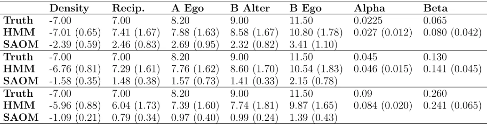
4.3 Simulation study results . . . 64
4.4 Root mean squared error and relative efficiency for the SAOM param-eter estimates . . . 64
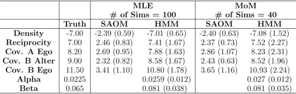
4.5 Mean and standard deviation of parameter estimates for MLE vs. MoM for estimation ofθ. . . 65
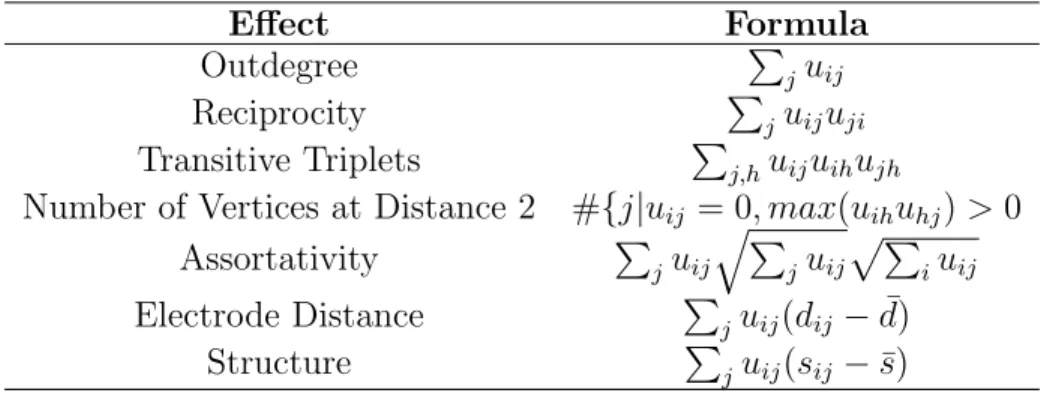
4.6 Mathematical definition of SAOM effects for EEG functional network analysis . . . 71
4.7 EEG functional network analysis results . . . 73
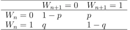
5.1 ER transition probability matrix . . . 78
5.2 Counts corresponding to type I and type II errors . . . 84
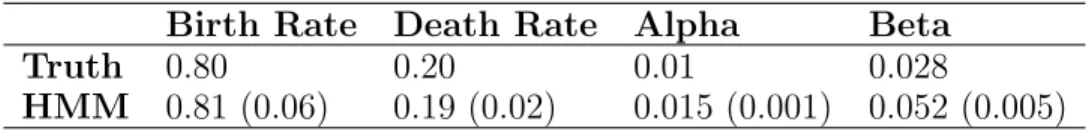
5.3 Mean and standard deviation of parameter estimates based off of 10 simulations . . . 88
3·1 Flow chart of proposed framework for longitudinal complex brain
net-work analysis. . . 12
3·2 Visual depiction of SAOM periods . . . 27
4·1 Hidden Markov model set-up . . . 42
4·2 Particle filtering sampling scheme . . . 53
4·3 High probability adjacency matrix . . . 61
4·4 Boxplots for density and reciprocity parameter estimate distributions 66 4·5 Boxplots for Covariate B alter and ego parameter estimate distributions 67 4·6 Boxplots for Covariate A ego parameter estimate distributions . . . . 67
5·1 Error-free Erd˝os-R´enyi birth and death process . . . 80
5·2 Error-free Achlioptas’ birth and death process . . . 81
5·3 ER and PR birth and death process with noise . . . 81
B·1 Mean value of three cycles parameter over time . . . 98
B·2 Mean value of between parameter over time . . . 99
B·3 Mean value of same lobe parameter over time . . . 100
B·4 Mean value of DMN parameter over time . . . 101
AD . . . Alzheimer’s disease
ADNI . . . Alzheimer’s Disease NeuroImaging Initiative BNT . . . Boston naming test
BOLD . . . Blood-Oxygen-Level dependent DMN . . . Default mode network
DTI . . . Diffusion tensor imaging EEG . . . Electroencephalogram EM . . . Expectation-Maximization ER . . . Erd˝os-R´enyi
HMM . . . Hidden Markov model
fMRI . . . Functional magnetic resonance imaging GCC . . . Giant connected component
ICA . . . Independent component analysis MCI . . . Mild cognitive impairment MLE . . . Maximum likelihood estimation MMSE . . . Mini-mental state examination MOM . . . Method of moments
PET . . . Positron emission tomography PR . . . Achlioptas’ product rule ROI . . . Region of interest
rsfMRI . . . Resting-state functional magnetic resonance imaging SAOM . . . Stochastic actor-oriented model
TERGM . . . Temporal exponential random graph model
Chapter 1
Introduction
The study of complex brain networks, where the brain can be viewed as a system with various interacting regions that produce complex behaviors, has grown tremendously over the past decade. Networks are becoming a popular model to illustrate both the physiological connections (structural networks) and the coupling of dynamic brain activity (functional networks) linking different areas of the brain. It is within this paradigm shift that scientists have begun investigating how complex networks behave in healthy brains and how they are altered in neurological and psychiatric disorders [Stam, 2014].
Much of the statistical network science tools for analyzing complex brain networks have been developed for cross-sectional studies and for the analysis of static networks. However, with both an increase in longitudinal study designs, as well as an increased interest in the neurological network changes that occur during the progression of a disease, more sophisticated methods for longitudinal brain network analysis are needed. In this dissertation, we propose multiple methods for the analysis of complex networks in neuroscience, and we demonstrate the applicability of our methods on a variety of brain network data. The layout is as follows.
The second chapter provides some background information on Stochastic actor oriented models (SAOMs) [Snijders et al., 2010b]. Originally developed in the social network context, they are a type of model for the purpose of representing network dynamics. Much of this dissertation focuses on either adapting these models to a
neuroscience setting or extending these models.
The third chapter focuses on a longitudinal brain network analysis of resting-state fMRI complex functional networks obtained from participants in the Alzheimers Dis-ease Neuroimaging Initiative (ADNI) [Mueller et al., 2005]. In performing this analy-sis, we propose a framework for the longitudinal analysis of complex brain networks. Furthermore, this framework has significant potential to be used in many applica-tions, in addition to resting-state data in our Alzheimers disease (AD) study. At the heart of the proposed framework is the adaptation of SAOMs to the neuroscience setting. Originally developed in a social network context, these models had not been previously applied in neuroscience. SAOMs model networks over time as longitudinal observations of a continuous-time Markov chain on network space. Network dynam-ics are represented as being driven by various factors, both endogenous (i.e., network effects, such as triangle formation) and exogenous, where the latter include potential mechanisms and relationships conjectured in the literature. For example, one could test whether regions of interest (ROIs) in the same lobe have more of a tendency to connect or whether certain ROIs that are known to be hubs in the sense that they connect many different areas of the brain tend to lose connections during AD. We draw illustrative conclusions at the subject level, and then we perform a meta-analysis to conduct a comparison between elderly controls and individuals with AD.
The fourth chapter is motivated by the work of the third chapter. The current SAOM framework assumes the observed network edges are free of type I and type II error. However, in some settings (such as in a brain network setting), this is an unrealistic assumption. We propose a hidden Markov model (HMM) based approach to estimate the error and the parameters in the SAOM. The modeling approach con-sists of two components: 1) the latent model, which assumes that the unobserved, true networks evolve according to a Markov process as they did in the original SAOM
framework; and 2) the measurement model, which describes the conditional distribu-tion of the observed networks given the true networks. An expectadistribu-tion-maximizadistribu-tion (EM) algorithm has been developed for estimation, with the incorporation of a parti-cle filtering based sampling scheme due to the enormity of the state space. We have performed a simulation study that shows our method offers substantial improvement in the accuracy of parameter estimates when compared to the nave approach of just fitting a SAOM. We also demonstrate our method on functional brain networks in-ferred from electroencephalogram (EEG) data, where we have structural connectivity deduced from diffusion tensor imaging (DTI) data as a predictor in our model, along with a measure of distance between nodes and several network structure based pre-dictors.
The fifth chapter pertains to the study of percolation - the sudden emergence of a giant connected component (GCC) in a network. This has become an active area of research, with relevance in clinical neuroscience. For example, epileptic seizures are associated with an explosion of connectivity across the brain [Kramer et al., 2010]. It is possible that the type of phase transition undergone during a seizure may have impact on the best treatment of epilepsy. This leads us to the important question: “How can we distinguish between different percolation regimes in practice?” We will build off of the work of [Viles et al., 2016], but with the goal of estimating a percolation model from a given sequence of observed networks with single edge transitions. The birth and death rates for the edges will need to be estimated, as well as the type I and type II error rates. Similar to the previous project, we are proposing an HMM based approach with an EM algorithm and particle filtering based estimation routine for computation.
Lastly, in Chapter 6, we close with a discussion on future research directions motivated by the work presented in this dissertation.
Chapter 2
SAOM Background
For Chapters 3 and 4, we adopt the stochastic actor oriented modeling framework by Snijders et al. for the evolution of complex networks, which are observed at moments m = 1, ..., M [Snijders et al., 2010b]. In this framework, it is assumed that the changing network is the outcome of a continuous time Markov process with time parameter t ∈T, where the u(tm) are realizations of stochastic digraphs U(tm) embedded in a continuous-time stochastic process U(t), t1 ≤ t ≤ tM. Let Ω be the node set, which is assumed to be the same for all observation moments. The totality of possible networks on Ω is the state space, and the discrete set of true networks are snapshots of the network state during this continuous period of time. In other words, many changes are assumed to happen sequentially between what is being observed, and the process unfolds in time steps of potential varying lengths [Snijders et al., 2010b].
When dealing with directed networks, which is the default in SAOMs, each U(t) is made up of |Ω| ×(|Ω| −1) possible edge status variables uij, where uij = 1 when there exists a directed edge from vertex i to vertex j and uij = 0 otherwise. There are |Ω|×(|2Ω|−1) edge status variables in the undirected case. At a given moment, one probabilistically selected vertex may change an edge, where the decision is modeled according to a random utility model, requiring the specification of a utility function (i.e. objective function) depending on a set of explanatory variables and parameters. Therefore, we are reduced to modeling the change of one edge status variable uij by
one vertex at a time (a network micro step) and modeling the occurrence of all of these micro steps over time. The first true networku(t1) serves as a starting value of the evolution process - the uij are conditioned upon. For each vertex i, the waiting time until vertexitakes a micro step is modeled by exponential distributions. At any time point t with current network u(t) = u, each of the vertices has a rate function λi(δ, u) where δ is a parameter. Therefore, the waiting time until occurrence of the next micro step by any vertex is exponentially distributed with parameter
λ(δ, u) = V X
i=1
λi(δ, u) (2.0.1)
Given that an opportunity for change occurs, the probability that it is vertex i who gets the opportunity is given by
πi(δ, u) =
λi(δ, u)
λ(δ, u) (2.0.2)
The microstep that vertexi takes is determined probabilistically by a linear com-bination of effects. For example, let’s assume thatuis the current network and vertex i has the opportunity to make a network change. The next network state u0 must either equal u or deviate from u by one edge. Vertex i chooses the value of u0 for which
fi(u, u0, γ) +i(u, u0) (2.0.3)
is maximal, wherei(u, u0) is a Gumbel-distributed random disturbance that captures the uncertainty stemming from unknown factors, and
fi(u, u0, γ) = X
e
γeSe(i, u, u0) (2.0.4)
where γe represent parameters and Se(i, u, u0) represent the corresponding effects. There are many types of effects one can place in the model. See [Ripley et al., 2011] for a full list. Some are purely structural effects, such as triangle formation and reciprocity. Other effects may involve vertex traits, such as gender or smoking status of the individuals in a social network.
Equation 2.0.4 is the objective function to which we have been referring. It can be thought of as a function of the network perceived by the focal vertex. Probabilities are higher for moving towards network states with a high value of the objective function. The objective function depends on the personal network position of vertex i, vertex i’s exogenous covariates, and the exogenous covariates of all of the vertices in i’s personal network. Due to distributional assumptions placed on i(u, u0), the probability of choosing u0 can be expressed in multinomial logit form as
exp(fi(u, u0, γ) P
u00
exp(fi(u, u00, γ))
(2.0.5)
where the sum of the denominator extends over all possible next network states u00.
For each set of model parameters, there exists a stationary distribution of prob-abilities over the state space of all possible network configurations. The complexity of the model does not allow for the equilibrium distribution nor the likelihood of the network ‘snapshots’ to be calculated in closed form. Therefore, parameter estimates are obtained either via an iterative stochastic approximation version of the Method of Moments approach or a Maximum Likelihood approach based on data augmentation
and stochastic approximation. The RSiena R package is used to estimate and fit the model [Ripley et al., 2011].
Chapter 3
Longitudinal Network Analysis in
Resting-State fMRI for Alzheimer’s
Disease
3.1
Introduction
Alzheimer’s disease (AD) is the most common neurodegenerative disorder, affecting millions of people worldwide and accounting for 60-80% of dementia cases. It is a progressive disease, where symptoms gradually worsen over a number of years. In its early stages, memory loss is the most salient feature, but in later stages, deficits spread to areas of cognition such as language, eventually inducing impairments of all cognitive functions [Win, 2015]. Currently, there is no cure for the disease, but there is a worldwide effort under way to develop additional agents to reduce the rate of progression, and ultimately, to prevent it from developing.
Resting-state functional magnetic resonance imaging (rsfMRI) is considered a promising biomarker for AD. It is a technique that focuses on spontaneous low fre-quency fluctuations (<0.1Hz) in the Blood-Oxygen-Level Dependent (BOLD) signal, and in contrast to task-based fMRI, it is often used to evaluate regional interactions in the brain that occur when a subject is not performing a task [Lee et al., 2013]. In particular, rsfMRI can detect abnormalities in complex functional brain networks where functional connections (connections that rely on the coupling between dynamic activity) are evaluated for all pairs of pre-specified brain regions of interest (ROIs) to
create an interconnected representation of the brain [Simpson et al., 2013]. In con-trast to other rsfMRI analytic methods that are more widely used (e.g. seed-based functional connectivity and independent component analysis), graph-based network analyses allow one to visualize the overall connectivity pattern among all ROIs, quan-titatively assess differences in global network structure, and investigate how different modules (i.e. interconnected clusters of ROIs) interact with one another [Simpson et al., 2013]. A great deal of evidence now supports the theory that the brain is a system of interacting regions that produce complex behaviors. Understanding brain development and causes of neurological disorders, such as AD, as well as developing more effective treatments, require not just gaining knowledge about separate com-ponents in the brain, but also studying how these comcom-ponents interact [Telesford et al., 2011, Sporns, 2014, Mesulam, 1990, Bressler and Menon, 2010]. It is within this paradigm shift that scientists have begun investigating how functional networks be-have in healthy brains and are altered in neurological and psychiatric disorders [Stam, 2014].
There are several reports in the literature on resting-state complex functional network changes in those with Mild Cognitive Impairment (MCI) and AD. For ex-ample, researchers have reported on changes in network characteristics such as path length, clustering, node centrality, hubs, and modularity [Greicius et al., 2004, Wang et al., 2010, Supekar et al., 2008]. However, most of what has been studied thus far has been at one time point on several global summary measures. The potential to conduct longitudinal complex network analysis remains largely untapped. With the growth of AD initiatives that are collecting and providing access to neuroimaging data over time on many subjects, such as the Alzheimer’s Disease Neuroimaging Initia-tive (ADNI) [Mueller et al., 2005] and the National Alzheimer Disease Coordinating Center (NACC) Database [Beekly et al., 2004], a natural next step is to assess
lon-gitudinal neurological network changes occurring during the progression of AD and to compare these disease-related changes to network changes in a cohort of healthy aging controls. We should note that longitudinal ‘network’ analyses have occasionally been performed, but the researchers define networks based on independent compo-nent analysis (instead of the graph theoretical approach that we are focused on here), and their analysis consists of only two time points [Bai et al., 2011,Damoiseaux et al., 2012].
In this chapter, we conduct a longitudinal brain network analysis on resting-state fMRI complex functional networks obtained from participants in ADNI. In doing so, we propose a paradigm for the longitudinal analysis of complex brain networks. Al-though we concentrate on rsfMRI functional networks, our paradigm can be used in various applications. The heart of the framework is the adaptation of SAOMs to the neuroscience setting. SAOMs are designed to capture network dynamics representing a variety of influences on network change in a continuous-time Markov chain frame-work [Snijders et al., 2010b]. In other words, they are designed to quantify and test the influence that specific traits of the ROIs or specific network structures have on which connections will form or dissolve. To the best of our knowledge, these models have not yet been used in neuroscience. Originally developed in the social network setting, SAOMs revolve around the notion that the ‘actors,’ or nodes in the network, are in control of the edges they create and dissolve over time. As described in chapter 2, the nodes make changes to edge status subject to an objective function; a linear combination of effects that can be either functions of the network itself (endogenous effects, such as triangle formation) or characteristics of the nodes themselves (ex-ogenous effects), with the latter including potential mechanisms and relationships conjectured in the literature. For example, an endogenous effect that one may wish to test is whether two ROIs are more likely to connect if they already have a
mu-tual connection with another ROI. An example of an exogenous effect one may test is whether ROIs involved in executive function are more likely to connect to other ROIs involved in executive function. Importantly, this framework lends itself to the testing of such hypotheses through the estimation of parameters expressing possible influences on network changes [Snijders et al., 2010b].
Given existing literature that indicates brain regions often change functional con-nections as a compensatory mechanism [Gardini et al., 2015, Etkin et al., 2009, Simp-son and Laurienti, 2015] or that ‘hub’ regions shift which regions they communicate with based on instructions for the task at hand [Cole et al., 2013], an ‘actor-oriented’ or ’node-oriented’ approach is well-motivated and appealing. Not only is this frame-work that we are proposing to analyze our data intended to model and draw inference from fully constructed longitudinal whole-brain networks, which is a novel contribu-tion in itself, but the models allow for a wide variety of hypotheses to be tested through the many effects that can be incorporated. In fact, in using SAOMs, we are able to assess the effect of a given mechanism while controlling for the possible simultaneous operation of other mechanisms or tendencies (e.g. clustering, ROIs in the same lobe connecting, etc), which may be competing and even complementary. With much of the existing literature on complex network analysis in neuroscience focusing on a single effect at a time, these models offer new insight by allowing for the adjustment and testing of multiple effects at once. This SAOM framework al-lows researchers to delve in, disentangle, and identify which mechanisms are driving network change over time (as opposed to focusing on different network characteris-tics individually), which is sure to offer new insights into processes involved in both normal brain development and also in various brain disorders.
Figure 3.1 outlines the framework we use to analyze our resting-state functional networks. We begin with rsfMRI data collection for i = 1, ..., N subjects over each
of their Mi longitudinal observation moments (e.g. study visits). The next stage is network construction, using one of the many methods existing in the literature; all of which are largely driven by the type of neuroimaging data being analyzed. After network construction, hypotheses must be formalized and paired with effects that can be placed into the SAOMs, and the models are fit to each individual subject’s longitudinal series of networks. The final step is to perform a meta-analysis on the model output, allowing one to formally test a number of current hypotheses and draw conclusions at the group level. Each of these steps requires careful attention, and the real challenge lies in formulating hypotheses and creating effects in ways that are both statistically sound and well grounded in neuroscience theory.
In Section 3.2, we describe each of the above steps in more detail in the context of our study and data. Then, in Section 3.3.1, we report illustrative results for two of our subjects. In Section 3.3.2, we present the results of a meta-analysis where we formally test a number of current hypotheses in the AD literature. Lastly, we end with a brief discussion in Section 3.4.
Figure 3·1: Flow chart of proposed framework for longitudinal com-plex brain network analysis.
3.2
Methods
3.2.1 Subjects and fMRI Subjects
Data used in the preparation of this article were obtained from the ADNI database (adni.loni.usc.edu). The ADNI was launched in 2003 as a public-private partnership, led by Principal Investigator Michael W. Weiner, MD. The primary goal of ADNI has been to test whether serial MRI, positron emission tomography (PET), other biological markers, and clinical and neuropsychological assessment can be combined to measure the progression of MCI and early AD. ADNI was originally slated as a 5 year endeavor, but was extended by a 2-year Grand Opportunities grant in 2009 and a renewal of ADNI (ADNI-2) in October 2010 through to 2016, with enrollment of an additional 550 participants [Mueller et al., 2005]. For up-to-date information, see www.adni-info.org.
All of our subjects are participants of ADNI-2. ADNI-2, in general, has subjects who are classified as having normal cognitive status, MCI, or AD. Subjects were as-signed to a diagnostic group by ADNI site investigators at screening and baseline visits. Subjects also had data collected over a series of visits that include screen-ing/baseline, 3 months, 6 months, one year, and occasionally two years. Resting-state fMRI data are known to contain a substantial amount of noise, related to factors like cardiac and respiratory signals [Lee et al., 2013]. Additionally, the number of sub-jects with resting-state fMRI scans was somewhat limited due to the selection criteria employed. Accordingly, in order to maximize the ratio of signal to noise, we chose to focus on a comparison of two extremes, selecting patients who are of either normal cognitive status (controls) or who have been classified as having AD (cases). When selecting subjects, we only chose those that had at least two visits with resting-state fMRI scans, and additionally, we tried to limit the number of subjects who had
non-monotone missingness (i.e. subjects who have missing observations and then return and have non-missing information at a later time point). With these inclusion criteria, we have a sample of 25 controls and 21 cases.
Resting-state fMRI
Functional communication between brain regions is highly important in complex cog-nitive mechanisms, and resting-state fMRI (rsfMRI) has drawn much interest in recent years. In the past, functional communication was typically looked at in fMRI using task-based or stimulus-driven paradigms, while fMRI at rest was interpreted to have no meaning and was just ‘background noise’. However, it is now widely recognized that the brain is never silent [Sporns, 2013]. Rather, it is always engaged in anatom-ically structured and meaningful neural activity, and is shown to not only be altered in neurological or psychiatric diseases, but also during healthy aging [Damoiseaux et al., 2008, Andrews-Hanna et al., 2007, Mathys et al., 2014]. Resting-state fMRI also has its advantages in that it allows functional data to be acquired in patients with a wide range of cognitive abilities, it avoids performance related variability of ac-tivation fMRI studies, and it is less complicated to acquire and standardize [Fleisher et al., 2009].
Data Acquisition and Pre-processing
Structural scans were acquired on 3T Phillips System scanners using the 3D MPRAGE protocol and rsfMRI protocol developed by ADNI (http://adni.loni.usc.edu/methods/ documents/mri-protocols/). The MPRAGE scans were acquired in the sagittal plane using the following parameters: TR/TE 3000/4 ms; flip angle 8◦ - 9◦; section thick-ness 1.2 mm; 170 sagittal slices. Functional data were acquired while subjects focused on a dot in the middle of the screen, per the ADNI protocol. The rsfMRI sequence consisted of a seven-minute functional run acquired in the axial plane using a
T2*-sensitive gradient-recalled, single-shot echo-planar imaging pulse sequence (TR/TE 3000/30 ms, FoV = 212 mm, flip angle 80◦, matrix size 64 × 64, inplane resolution 3.3 mm ×3.3 mm). Each volume consisted of 48 slices parallel to the bicommissural plane (slice thickness 3.3 mm, no gap), and each functional run was comprised of 140 volumes.
Freesurfer software (surfer.nmr.mgh.harvard.edu version 5.3) was used to par-cel and label the structural MPRAGE scans of each of the subjects [Desikan et al., 2006]. The software identified grey matter regions in the cortex and sub-cortex. The results were checked for accuracy manually. Sixty-four grey matter regions of inter-est (ROIs) from the cortex and sub-cortex were chosen from these labels, excluding those highly susceptible to field distortions. Please refer to Appendix A for a full list. All of the rsfMRI scans were visually inspected to ensure that they were free from any artifacts (i.e. pencil beam artifact). No scans were excluded due to ar-tifact. The fMRI data were preprocessed with motion correction using MCFLIRT, spatial smoothing with a kernel size of 5 mm, and highpass temporal filtering us-ing a local fit of a straight line. FMRI Expert Analysis Tool (FEAT; Oxford, UK; v6.0 http://fsl.fmrib.ox.ac.uk/fsl/fslwiki/FSL) was used for this preprocessing [Smith et al., 2009]. Each rsfMRI sequence was registered to the brain image extracted from the structural scan by Freesurfer and the resulting rsfMRI sequence was labeled using the generated Freesurfer ROIs. A mean time series for each ROI was calculated by averaging all fMRI voxel values within each ROI over time, resulting in 140 time points calculated for each 7 minute resting state session.
3.2.2 Construction of Brain Networks
We define our functional connection matrix, or |Ω| × |Ω| adjacency matrix of edge status variables (uij), obtained for each subject at each of his/her scans to be an undirected binary graph G with |Ω|= 64 nodes. An edge between verticesi and j is
defined as uij = 1. The edges in the network represent binary undirected functional connections between regions. To estimate each connection matrix, we first calcu-lated the Pearson Correlation matrix, where Pearson correlation between two ROIs is defined as ρ= P (yn−y)(z¯ n−¯z) √ P (yn−y)¯2P(zn−z)¯2
where ρis the Pearson correlation coefficient and ¯y and ¯z are the mean values of the BOLD signal time courses for ROIs y and z respectively. We decided on Pearson correlation when defining edges given that there is some evidence that, via Test Re-test analyses, the reliability is highest for Pearson’s-correlation-based brain networks [Liang et al., 2012]. Please see the discussion section for additional information.
Next, we took the top 20% of Pearson correlation values and defined their corre-sponding edge status variables to be 1 (i.e. a functionally connected node pair). As is standard in the literature, we chose to work with positive correlations only [Schwarz and McGonigle, 2011, Rubinov and Sporns, 2010]. Such thresholding led to equal edge densities in all subjects and time points, which is important for comparisons of network topology. In addition, we chose a 20% edge density to be in line with what would be expected from the edge density of the underlying structural connectivity which ranges from 10−30% [Van Wijk et al., 2010]. Out of the 184 total networks in our analysis, 162 of them are connected as a single connected component at the 20% threshold. Of the 22 networks that are not completely connected, 14 have only one ROI that is not included in the giant connected component, and the remaining 8 all have a very large connected component.
3.2.3 Stochastic Actor-Oriented Models Hypotheses and Effects
The specification of a SAOM is done by defining a rate function and an objective function. The rate function indicates the speed at which the ROIs obtain an oppor-tunity to change a connection, while the objective function informs which changes are made when given the opportunity. Following the recommendation of SAOM docu-mentation, we used a constant rate function without additional rate function effects, but it is possible to let the rate function depend on individual ROI covariates when there are important size or activity differences between them. The objective function we will use involves effects that we have matched to hypotheses we wish to test. We have outlined each hypothesis we wish to test below, along with its matching effect(s). It is important to keep in mind that for these models, hypotheses and effects can be made based on functions of the network topology itself (i.e. endogenous effects), at-tributes related to pairs of ROIs (dyadic exogenous effects), and atat-tributes related to individual ROIs (monadic exogenous effects).
Endogenous Hypotheses and Effects
Clustering Hypothesis: Clustering is an indication of segregation in the network. The clustering coefficient of a vertex is calculated as the ratio of the number of existing edges between its neighbors and the total number of possible edges. The global clustering coefficient of a network is computed by averaging the clustering coefficient of all vertices of the graph, reflecting, on average, the prevalence of clustered connectivity around individual nodes [Kolaczyk, 2009].
Network analysis of functional connectivity data for healthy individuals has been characterized by a high clustering coefficient, which is associated with high local efficiency of information transfer for specialized processing [Schulz et al., 2014]. It is of
interest to investigate whether this holds in people with AD. Sanz-Arigita et al. found no difference in the clustering coefficient in resting-state functional networks between AD patients and healthy age-matched controls [Sanz-Arigita et al., 2010]. Whereas, in another resting-state fMRI experiment, Supekar et al. found that the clustering coefficient was significantly decreased in AD, specifically in bilateral hippocampus, and could be used to distinguish AD participants from controls with high specificity and sensitivity [Supekar et al., 2008].
In our study, we look at differences in clustering between cases and controls by comparing their tendency to form triangles. Not only are triangles a good represen-tation of clustering, but they are important from a motif standpoint. Network motifs are of interest because they represent different topological patterns of connections, or “building blocks” of the network as a whole [Sporns, 2011, Sporns, 2013].
Three-cycles Effect- The tendency of ROIs to connect in a triangular pattern. P
j,huijujhuhi
Integration Hypothesis: Another structural characteristic that is often looked at hand-in-hand with clustering is average shortest path length, a measure of integration. The shortest path length between nodesiandj(also called distance or geodesic path) is defined as the minimum number of edges that must be traversed to go from node i to node j. Short path lengths promote functional integration and efficiency since they allow for communication with few intermediate steps, minimizing effects of noise or signal degradation [Sporns, 2013].
Studies have shown that functional networks in AD have longer path lengths -indicating a less efficient organization of the connectivity. For example, Sanz-Arigita found that, compared to controls, the average path length of AD resting-state func-tional networks is closer to the theoretical values of random networks [Sanz-Arigita et al., 2010]. Moreover, in their study, Xiang et al. analyzed brain networks using
ADNI resting-state fMRI data that was extracted from normal controls, patients with early MCI, patients with late MCI, and patients with AD. They found that as cogni-tive deficits increased across the four groups, the shortest paths in the resting-state functional network gradually increased as well [Xiang et al., 2013]. Similarly, we would also like to investigate the notion of distance between ROIs and conduct a comparison between our cases and controls. We have two effects related to distance.
Number of Distances 2 Effect - Defined by the number of ROIs to whom i is indirectly tied (through at least one intermediary). When this effect has a negative parameter, ROIs will have a preference for having few others at a geodesic distance of 2.
#{j|uij = 0, maxh(uihuhj)>0}
Between Effect- The tendency for ROIs to position themselves between other ROIs that are not directly connected to one another.
P
j,huhiuij(1−uhj)
Lastly, the following endogenous effect is typically included in all SAOMs to account for the observed density of the networks, so we chose to include it as well. It represents the basic tendency of ROIs to make connections to other ROIs.
Degree Effect: P
juij (where i, j are vertices and uij = 1 if there is an edge connecting i and j and 0 otherwise).
Exogenous Hypotheses and Effects
Segregation Hypothesis: Functional segregation is another concept that appears quite frequently in the neuroscience literature. Functional segregation in the brain is the capability for specialized processing to occur within densely interconnected groups of regions, called clusters or modules [Rubinov and Sporns, 2010]. Modules permit quick and efficient sharing of information among brain regions that tend to work together towards a common set of goals, while adhering to their functional specializa-tion and limiting the spread of informaspecializa-tion across the entire brain network [Sporns, 2013]. A network’s modular structure is identified (sometimes called community de-tection) by partitioning the network into groups of nodes, with a greater number of within-group links, and a lesser number of between-group links [Kolaczyk, 2009]. Unlike most other network measures, the optimal partitioning for a given network is typically estimated with optimization algorithms, so results tend to vary depending on study designs and community detection procedures used [Danon et al., 2005].
In their analysis, Salvador et al. constructed resting-state fMRI networks from average partial correlation matrices from healthy volunteers and found that significant connections were often local, involving regions in the same lobe and/or closely adja-cent to each other anatomically [Salvador et al., 2005]. They went on to perform a hi-erarchical clustering analysis of healthy controls, revealing that the basic hierarchy of brain functional organization tends to be designated as lobar/sublobar/symmetrical. In other words, ROIs in the same lobe tend to have more connections between each other, with symmetrical links between bilaterally homologous regions consistently expressed at the lowest level of the hierarchy [Salvador et al., 2005].
We would like to control, at the very least, for the fact that ROIs tend to be connected to ROIs that are anatomically close to them, but we would also like to explore whether this modular, efficient network structure that is found in healthy
individuals, tends to break down in people with AD. Given that there is not one standard set of partitions for the ROIs, and given the results of Salvador et al, we define groups according to cortical lobes, with the following effect:
Same Lobe Effect- A dyadic effect to represent the tendency for ROIs in the same lobe to connect. This is our modularity effect.
P
juijI{ai =aj} where ai indicates the lobe for ROI i.
We would also like to account for the notion that symmetrical links between bilaterally homologous regions might be more likely to be connected through the following dyadic effect:
Bilateral Effect: P
juij(bij −¯b) where bij = 1 if two ROIs are bilaterally homolo-gous and bij = 0 otherwise
Default Mode Network Hypothesis: The final question we would like to address in our study involves the Default Mode Network (DMN), a network of interacting brain regions known to have activity highly correlated with one another in resting state functional networks and much less activity during any attention-demanding task. Although the exact role of the DMN remains unknown, it is thought to be involved in monitoring internal stimuli, as well as in maintaining consciousness [Greicius et al., 2003, Wicker et al., 2003].
In AD, the DMN is thought to be affected by reduced functional connectivity and atrophy. For example, Sorq et al. analyzed fMRI data from healthy individuals and patients with high risk for developing AD and found that select areas of the DMN showed reduced connectivity in the patient group [Sorg et al., 2007]. Several other studies have also reported similar findings [Greicius et al., 2004, Wu et al., 2011]. Often times the default mode network is identified via independent component anal-ysis (ICA). ICA separates time course data into a collection of independent signals,
or components, (without an explicit model) where each component represents a ‘net-work’ following a similar temporal pattern [Moussa et al., 2012]. Since our framework is more hypothesis-driven, as opposed to data-driven, we must identify DMN ROIs prior to modeling and testing. Given that there is some evidence in the literature that resting state networks (RSNs) identified via graph-based network analyses are comparable to the corresponding RSNs identified by ICA, with the DMN being one of the most robust [Moussa et al., 2012], we elect to define DMN ROIs in this manner. Therefore, we choose to specifically define DMN ROIs to be each of the following in both the left and right hemispheres of the cerebrum: caudal and rostral anterior cin-gulate, inferior parietal, middle temporal, posterior cincin-gulate, and precuneus, as these seemed to be the most consistently identified DMN ROIs in the literature [Buckner et al., 2008, Laird et al., 2009, van den Heuvel et al., 2009]. We hypothesize that con-nections between these ROIs will be less likely to exist in cases, compared to controls. It should be noted that there is much debate on which ROIs make up the DMN, so while we have decided to use this specific set of ROIs for our primary analysis, other choices can be argued as well. In fact, we perform a secondary analysis where we slightly modify this set of DMN ROIs. Both sets of results are reported in section 3.2
DMN Effect- A dyadic effect for the tendency of DMN ROIs to be densely connected to one another.
P
jxij(wij −w¯), where wij = 1 if two ROIs are in the DMN we have defined and wij = 0 otherwise
Model Specifications
We fit a SAOM with all of our effects (objective function shown below) separately, for each pair of consecutive time points and for each of our 46 subjects. This is effectively performing a sliding window analysis due to the potential non-stationarity
of our networks. Therefore, a subject will have Mi −1 sets of parameter estimates where Mi is the number of visits they had rsfMRI scans.
fi(g, g0, θ) = θ0 X j uij +θ1 X j,h uijujhuhi+θ2#{j|uij = 0, maxh(uihuhj)>0} +θ3 X j,h uhiuij(1−uhj) +θ4 X j uijI{ai =aj}+θ5 X j uij(wij −w¯) +θ6 X j uij(bij−¯b)
Our model parameters were all estimated using Method of Moments, the default approach, under the standard options of RSiena (i.e. estimation of the parameters is based on 4 consecutive and increasingly accurate subphases of the Robbins-Monro moments estimation algorithm), and standard errors are calculated based on 1000 additional simulation runs. Lastly, all t-ratios for convergence associated with the individual parameters in our models are less than 0.1 in absolute value, indicating excellent convergence [Ripley et al., 2011].
3.2.4 Meta-Analysis
After applying the SAOMs on a subject-by-subject basis, in order to aggregate and contrast the findings from all our ADNI subjects and conduct a group level analysis, we perform a separate meta-analysis on each parameter. Standard meta-analysis approaches [DerSimonian and Laird, 1986, Normand, 1999] are not sufficient since we have multiple estimates for each parameter (one for each pair of consecutive time points) for each subject. Therefore, we perform a ‘longitudinal’ meta-analysis by fitting a general linear mixed effects model with some slight modifications [Ishak et al., 2007].
collected on subjects i = 1, ..., N. We denote by yi the Pi × 1 vector of observed estimates from the ith subject and by yij the jth observation from this subject. The simplest way to account for the correlation between estimates of the same individual is to allow a random-effect that is common to estimates of the same person. Therefore, the general linear mixed effects model is given by:
yij =β0+β1xi+β2pij +β3xi×pij +δi+εij (3.2.1) where β0 is a fixed intercept, β1 is a fixed slope for case/control status,β2 is a fixed slope for time period number, β3 is a fixed slope for the interaction between disease status and time period, xi = 1 for cases and xi = 0 for controls, pij indicates the time period number (i.e. pij = 1,2,3 or 4, where pij = 1, for example, represents the estimate obtained from fitting the SAOM model to a subject’s first network to their second network) and δi is a random intercept. We make the assumption that δi follows a normal distribution with mean 0 and variance D, while εi follows a multivariate normal distribution with mean 0 and variance Si (where Si is a Pi × Pi diagonal matrix with values set to the variances of estimates obtained for each person). We also assume that cov(εi, δi) = 0 and that observations from different subjects are independent, so thatcov(εij, εkl) = 0 wheni6=kand for any observations j, l. Therefore, the variance of the marginal distribution of yij is D +Sij, while the covariance between two estimates collected at times j and l from subject i is cov(yij, yil) =D.
For each of our models, we collected the parameter estimates of our 6 effects and fit the meta-analysis in (2.1) for each effect (separately). The models were estimated by maximum likelihood, using SAS 9.3 and the MIXED Procedure [Singer, 1998]. If we found the interaction to be non-significant at a conservativeα = 0.15 significance level, we removed it from the model and re-ran the analysis. If the parameter for
time was then also found to be non-significant at an α = 0.05 significance level, we went ahead and removed it and re-ran the analysis so that disease status was the only fixed effect in the model.
3.3
Results
3.3.1 Single Subject
As previously mentioned, our SAOMs must be fit on each individual. A model can be fit to an individual’s entire longitudinal sequence. However, due to potential heterogeneity of the influence of our effects, we chose to fit the models to each pair of consecutive networks in the series (Figure 3.2). For illustrative purposes, in Tables 3.1 and 3.2 we show the results for two subjects. Both are 74 year old females, but they differ in disease status.
It is important to note that the parameter estimates allow for a caricature of the rules governing the dynamic change in the network [Steglich et al., 2006]. Because the temporal progression is taken care of by the rate functions, the parameters in the objective function are static and are comparable across periods of different lengths of time. And, as the SAOM authors point out [Steglich et al., 2006], a common misun-derstanding is that the parameter estimates express tendencies over time. Instead, they should be interpreted as satisfaction measures that are suitable for explaining the observed changes.
The parameter estimates for the appearance of three-cycles have relatively large t-ratios (ratio of estimate to standard error) across all time points for both subjects. We must interpret individual analyses cautiously based on relative magnitude of t-ratios, as formal grounds for comparison to the t distribution are not well established. The estimate for three-cycles is also positive in all cases, indicating that triangle formation is favored as these networks evolve, controlling for the other effects in the
model. This suggests a preference for local clustering. Looking closely at the effect sizes, we see that the individual with AD has slightly smaller parameter estimates overall, compared to the healthy individual, leading us to wonder whether this is an indication of clustering breaking down in AD.
The distance two effect expresses network closure inversely. In all cases, we see a negative parameter estimate (with a relatively large corresponding t-ratio), mean-ing that ROIs have a preference for formmean-ing connections to few other ROIs with a distance of 2, controlling for the other effects. Another related effect is the between effect, which represents brokerage, or the tendency for ROIs to form edges that bridge gaps. The negative parameter estimates for this effect for both individuals, suggest avoidance of bridging gaps. This, combined with clustering tendencies leads to insular network structures.
As expected, our results consistently show a very strong tendency for ROIs to prefer forming connections to their symmetric counterpart in the opposite cortical hemisphere, and this doesn’t differ between our case and control. Moreover, the positive parameter estimate for our same lobe effect tells us that ROIs in the same lobe are more likely to have a functional connection than ROIs that are not in the same lobe, after adjusting for the other effects in the model.
Lastly, we see a fairly strong positive parameter estimate for our DMN effect for our healthy subject, but the individual with AD either has less strong positive estimates or negative estimates. This suggests that the subject with normal cognitive status has a higher probability of forming a functional connection between two DMN ROIs than between two ROIs that are not both apart of the DMN, controlling for the other effects in the model. However, we cannot say the same for the individual with AD.
Figure 3·2: An example of the periods the SAOMs are fit to for individuals.
28 Period 1 Period 2 Period 3 Period 4
Effect Est SE T-Ratio Est. SE T-Ratio Est SE T-Ratio Est SE T-Ratio Degree -0.1149 0.1586 -0.724 0.3070 0.2667 1.151 -0.2410 0.1727 -1.395 -0.4645 0.1911 -2.431 Three-Cycles 0.1151 0.0175 6.577 0.1285 0.0227 5.670 0.1497 0.0207 7.249 0.1037 0.0188 5.520 Distance 2 -0.1991 0.0366 -5.436 -0.1117 0.0403 -2.776 -0.1288 0.0355 -3.625 -0.2164 0.0412 -5.255 Betweenness -0.1130 0.0185 -6.099 -0.1777 0.0307 -5.779 -0.1168 0.0173 -6.730 -0.0508 0.0204 -2.488 Bilateral 1.8491 0.4156 4.449 1.4669 0.4599 3.189 1.3327 0.4099 3.251 1.1135 0.3820 2.915 Same Lobe 0.3882 0.0875 4.436 0.2921 0.1027 2.843 0.3283 0.0883 3.720 0.1560 0.1061 1.471 DMN 0.3362 0.2232 1.506 0.5218 0.2585 2.019 0.9925 0.2179 4.555 0.2501 0.2461 1.016
Table 3.2: Results for 74 year old female with AD
Period 1 Period 2 Period 3 Period 4
Effect Est SE T-Ratio Est. SE T-Ratio Est SE T-Ratio Est SE T-Ratio Degree -0.1044 0.2018 -0.5173 -0.7255 0.2186 -3.3188 -0.0467 0.2463 -0.1896 0.3309 0.2558 1.2936 Three-Cycles 0.0955 0.0173 5.5203 0.1000 0.0189 5.2910 0.1817 0.0147 12.3605 0.0733 0.0169 4.3373 Distance 2 -0.1785 0.0352 -5.0710 -0.2994 0.0412 -7.2670 -0.1778 0.0305 -5.8295 -0.2333 0.0346 -6.7428 Betweenness -0.1112 0.0193 -5.7617 -0.0478 0.0217 -2.2028 -0.1114 0.0249 -4.4739 -0.1678 0.0288 -5.8264 Bilateral 2.0173 0.4759 4.2389 1.4326 0.3897 3.6762 0.4000 0.2386 1.6764 3.4913 0.6810 5.1267 Same Lobe 0.1700 0.0747 2.2758 0.4618 0.0893 5.1713 0.1658 0.0925 1.7924 0.3161 0.0841 3.7586 DMN 0.0262 0.2602 0.1007 -0.2263 0.2645 -0.8556 0.1349 0.2224 0.6066 -0.3452 0.4799 0.7193
3.3.2 Meta-Analysis
Baseline descriptive statistics are reported in Table 3.3. Our control subjects show no signs of depression, MCI or dementia, with an average Boston Naming Test (BNT) score of 29 and an average Mini-Mental State Examination (MMSE) score of 29. AD participants have been evaluated and meet the NINCDS/ADRDA criteria for probable AD [23] and have an average BNT test score of 24 and an average MMSE score of 22. Our cases and controls did not significantly differ in age (p-value= 0.8698) or gender (p-value= 0.5683).
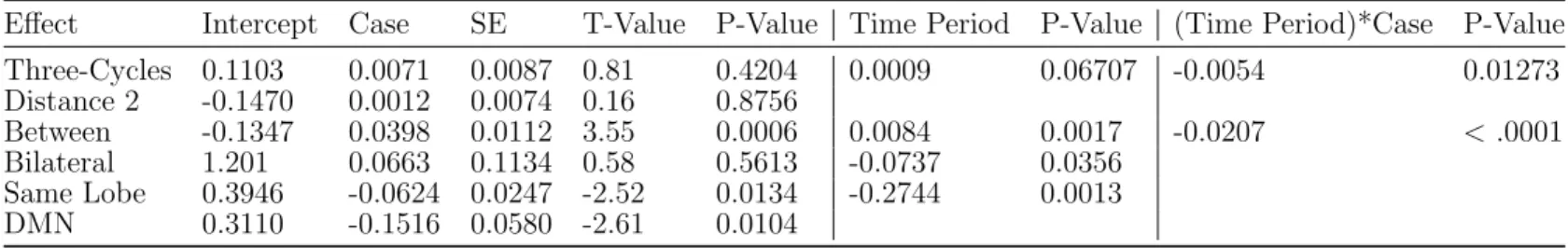
The primary meta-analysis results are shown in Table 3.4. Both the DMN effect and the same lobe effect substantially differ between cases and controls. Controls have a positive DMN parameter estimate, indicating a tendency of DMN ROIs to form connections with one another (p-value< .0001). However, cases show a significant decrease at the α=.01 level in the estimate (p-value= 0.0104). Controls also have a positive parameter estimate for the same lobe effect, indicating that ROIs in the same lobe have a higher probability of forming a connection (p-value< .0001). Meanwhile, cases show a significant decrease in the estimate (p-value= 0.0134) at the α = .05 significance level. Both cases and controls also show a decrease in the same lobe effect estimate over time (p-value= 0.0013).
The bilateral effect is positive, indicating a preference for bilaterally homologous ROIs to connect. However, the effect declines over time in both cases and controls (p-value= 0.0356). The negative distance 2 parameter suggests that ROIs tend to shy away from forming connections where they have a geodesic distance of at least 2 with other ROIs.
Both the between effect and the three-cycles effect have a significant interaction at the α=.15 level between disease status and time period, which makes it difficult to interpret the main effects of disease status and time period. Figures B1 and B2
in Appendix B show the mean value of each effect over time, and we can see that there does appear to be a qualitative interaction. The AD subjects have larger effects than the controls at their earlier time points but smaller effects than the controls at the later time points. Both groups appear to decline over time with respect to the three-cycles effect, but for the between effect, the controls have an increased effect over time, while the cases have a decreased effect. Again, it is difficult to interpret these results because of the strong interaction.
As noted in Section 3.2.3, there is some disagreement in the literature on which ROIs constitute the DMN. Therefore, we have performed a secondary analysis where we have modified which ROIs we have assigned as DMN ROIs. In this analysis, we no longer define the caudal anterior cingulate as a DMN ROI, and we add the superior frontal as a DMN ROI. We keep the remainder of the DMN list (as defined in section 3.2.2) the same. The results of this analysis are displayed in Table 5. We again find a significant interaction between disease status and time period for the three-cycles and between effects (plots are shown in Figures S1 and S2 in the supplement). We are no longer seeing a decrease over time for the bilateral effect at the α =.05 significance level, so time has been removed from that model. Probably the most notable change in this analysis is that both the DMN and same lobe effects now have a significant interaction between disease status and time period at the α =.10 significance level. The mean values of each over time (for both the primary and secondary analysis) are shown in Figures B3 and B4 in Appendix B. This gives a clearer picture of what is happening and one can see that the results actually do not end up looking so different from the primary analysis. The same lobe effect decreases over time for both cases and controls in both analyses, and the controls have larger effects over time compared to the cases in both. For the DMN effect, time does not appear to play much of a role (i.e. the change in the effect over time is minimal) and controls do
appear to consistently have larger effect values than cases. The trends aren’t quite as parallel in the secondary analysis as they were in the first, which is why we are seeing a potential interaction in the numerical results. However, as can be seen from the plots, the interaction is more quantitative than qualitative. If we remove the interaction, we still see a difference in the DMN and same lobe effects in cases versus controls but the p-values aren’t quite as small (p-values = .07 and 0.18, respectively).
We should also note that if we adjust for multiple comparisons using, for example, a Bonferroni adjustment(although one could look at False Discovery Rate, as well), we find no significant differences between our AD and control groups in either of our sets of analyses. We attribute this lack of significant difference after adjustment to the relatively small sample size in our study, as well as the high level of noise that is typically present in resting-state fMRI data. As an illustration of a sample size calcu-lation in this context, we have gone ahead and performed a rough power calcucalcu-lation to determine approximately what sample size would be needed for the case/control parameter estimate associated with the DMN effect outcome to be significant at the α = 0.05/6 = 0.0083 level (i.e. the Bonferroni adjusted α level assuming our main interest is in the case/control estimates). Assuming an effect size of 0.16 (based off of our primary analysis), 80% power, 3 observations per subject, and a conservative correlation of 0 among repeated measures, one would need a total sample size of ap-proximately 190 subjects. If we increase the correlation among repeated measures to be 0.4 (which is much larger than what it estimated from our current data), the sample size drops to be 116. G* Power 3 was used for these calculations [Faul et al., 2007].
32 Controls (n=25) AD Cases (n=21) P-value
Age 73.4 ± 5.2 73.7 ±7.6 0.8698
Gender, n (%) of males 12 (48.0) 12 (57.1) 0.5683
Boston Naming Test (BNT) 28.6 ± 1.3 23.5 ±4.2 <.0001
Mini-Mental State Examination (MMSE) 28.6 ± 1.6 22.4 ±2.5 <.0001
Table 3.4: Meta-Analysis results for the primary analysis. Controls are the reference group and standard errors, t-values, and p-values in the first section of the table all correspond to the case/control parameter estimate.
Effect Intercept Case SE T-Value P-Value Time Period P-Value (Time Period)*Case P-Value Three-Cycles 0.1103 0.0071 0.0087 0.81 0.4204 0.0009 0.06707 -0.0054 0.01273 Distance 2 -0.1470 0.0012 0.0074 0.16 0.8756 Between -0.1347 0.0398 0.0112 3.55 0.0006 0.0084 0.0017 -0.0207 <.0001 Bilateral 1.201 0.0663 0.1134 0.58 0.5613 -0.0737 0.0356 Same Lobe 0.3946 -0.0624 0.0247 -2.52 0.0134 -0.2744 0.0013 DMN 0.3110 -0.1516 0.0580 -2.61 0.0104
Table 3.5: Meta-Analysis results for the secondary analysis. Controls are the reference group and standard errors, t-values, and p-values in the first section of the table all correspond to the case/control parameter estimate.
Effect Intercept Case SE T-Value P-Value Time Period P-Value (Time Period)*Case P-Value Three-Cycles 0.1042 0.0278 0.0097 2.87 0.0050 0.0021 0.3377 -0.0123 0.0014 Distance 2 -0.1414 -0.0002 0.0094 -0.03 0.9793 Between -0.1342 0.0373 0.0116 3.20 0.0019 0.0074 0.0066 -0.0169 0.0004 Bilateral 1.0475 0.0705 0.1125 0.63 0.5325 Same Lobe 0.3759 0.0333 0.0458 0.73 0.4686 -0.0174 0.0934 -0.0380 0.0311 DMN 0.2037 0.0521 0.1137 0.46 0.6477 0.0294 0.2673 -0.0796 0.0986
3.4
Discussion
In this chapter, we conduct a longitudinal brain network analysis on resting-state fMRI complex functional networks obtained from participants in ADNI. We take sev-eral existing hypotheses conjectured in the literature and map them to effects in the SAOM framework, with the goal of testing these hypotheses and estimating param-eters expressing their strength, while controlling for the other factors in the model. After running the model on each participant and obtaining individual results, we con-duct a meta-analysis comparing AD patients with healthy controls. Both the DMN effect and the same lobe effect substantially differ between the two groups. Controls have a positive DMN parameter estimate, indicating a tendency of DMN ROIs to form connections with one another, while cases show a decrease in the estimate, lead-ing us to conclude that DMN ROIs aren’t as likely to activate and connect to one another in those with AD. Controls also have a positive parameter estimate for the same lobe effect, indicating that ROIs in the same lobe have a higher probability of forming a functional connection. Meanwhile, again, individuals with AD have a de-creased tendency of ROIs to form functional connections with other ROIs in the same lobe. Both cases and controls also show a decrease in the same lobe effect estimate over time.
The paradigm we have proposed to analyze these networks can be used in many applications other than on resting-state data in our AD study. These initial analyses we have performed are meant to be a proof of concept that pave the way forward for testing, in other contexts various other specific hypotheses related to functions of the nodes (e.g. ROIs) and the connections they have formed. Given the increased inter-est in, and clinical implications of, analyzing brain networks over time, we feel that a modeling framework that has the ability to test hypotheses and draw inference from a series of structural and/or functional networks is quite useful to the neuroscience
community. The SAOMs that we propose adapting are extremely flexible in that they are able to represent network dynamics as being driven by many factors/influences. Furthermore, the models allow for the accounting of several different explanations of network change, which may be competing and even complementary. This allows for the testing of effects driving the changes, while controlling for other factors, which better enables researchers to delve in, disentangle, and identify which mechanisms are playing a role (as opposed to focusing on different network characteristics indi-vidually).
Temporal Exponential Random Graph Models (TERGMs) [Hanneke et al., 2010] are the other popular choice of models for longitudinal network analysis, and to the best of our knowledge, they have not been used in neuroscience. Both types of models have their pros and cons, and we feel that both can be argued to be useful and appropriate in the context of networks in neuroscience. However, given that SAOMs (a) take an “actor-oriented” approach where the vertices are driving the network changes and (b) model network changes (and we expect network changes given that AD is a progressively degenerative disease) we feel that SAOMs are a natural choice for a first attempt at a more sophisticated method for longitudinal network analysis in neuroscience. A more detailed theoretical and empirical comparison between the two types of models can be found here [Leifeld and Cranmer, 2015].
It should also be noted that the paradigm we propose can be modified at several stages of the analysis regime. For example, in addition to Pearson Correlation, one can use other methods of network construction. Methods for estimating functional connectivity between nodes fall into one of two categories: association measures and modeling approaches. Correlation and coherence are two examples of linear associa-tion measures, while nonlinear measures include mutual informaassocia-tion and generalized synchronization. Partial correlation is one of the more popular methods and falls
somewhat in the middle of the association measure/modeling spectrum. The Smooth Incremental Graphical Lasso Estimation (SINGLE) Algorithm [Monti et al., 2014] is one example of a partial correlation based method specifically designed to infer dynamic functional connectivity networks from fMRI data. The literature on mod-eling approaches remains sparse, though [Varoquaux et al., 2010] and others have made contributions. See [Simpson et al., 2013] for a survey. There is currently no gold standard, but the choice of method is largely driven by the type of neuroimaging data being analyzed and the hypotheses one is interested in testing. The method used clearly may affect results. However, we necessarily leave a large-scale assessment of this issue, in the context of our proposed method, to future work.
Not only is there flexibility in the types of network data, network construction methods, and hypotheses tested, but the specifications of the random effects model used to conduct the meta-analysis can also be adjusted. We have included two fixed effects in our models (for case/control status and visit number). However, one could easily incorporate various individual attributes, such as age and gender into the mod-els as well. Since we did not find a significant difference in cases and controls on these variables, we chose not to adjust for them.
Another way that the meta-analysis can be modified is through correlation struc-ture. Our current formulation assumes that between-subject heterogeneity affects the parameters at each time period in a given subject the same way. One could extend the model by allowing a random slope for time. In fact, for our DMN effect, we ran a random intercept model and a random intercept and slope model separately. We compared the goodness of fit of these two models using a likelihood ratio test and did not find a significant difference (χ2 = 1.8, df=1, p-value = 0.1797), indicating that it may not improve the model much, at least with this particular outcome. One could also attempt a multivariate meta-analysis which would take into account the