On Transformation Based Circular Density Estimators

(1)

On Transformation Based Circular Density

Estimators

Yuhan Cao

A Thesis

in the Department of

Mathematics and Statistics

Presented in Partial Fulﬁllment of the Requirements

for the Degree of Master of Science (Mathematics) at

Concordia University

Montr´eal, Qu´ebec, Canada

May 2018

c

(2)

CONCORDIA UNIVERSITY

School of Graduate Studies

This is to certify that the thesis prepared

By: Yuhan Cao

Entitled: On Transformation Based Circular Density Estimators and submitted in partial fulﬁllment of the requirements for the degree of

Master of Science (Mathematics)

complies with the regulations of the University and meets the accepted standards with respect to originality and quality.

Signed by the ﬁnal examining committee:

Examiner Dr. Arusharka Sen Examiner Dr. Wei Sun Thesis Supervisor Dr. Yogendra P. Chaubey Approved by

Chair of Department or Graduate Program Director

Dean of Faculty

(3)

Abstract

Estimation of the probability density function for circular data is an important topic in statistical inference. In this thesis, I would like to introduce two transformation based methods for estimating probability density function in this context. One is derived from traditional kernel density estimator and the other one comes from the Bernstein poly-nomial estimator (Chaubey, 2017). We know both of the kernel density estimator (Sil-verman, 1986) and Bernstein polynomial estimator (Babu, Canty and Chaubey, 2002) are appropriate for the case of linear data, transformation of circular data to linear data would bring extreme simplicity to estimation of probability density function in the case of circular data by back transformation. I will conduct a simulation study to compare these methods with respect to their global and local errors. We ﬁnd through our sim-ulation study that transformed kernel density estimator has a stronger ability to allevi-ate the boundary problems than transformed Bernstein polynomial estimator, however, their overall performance is pretty much similar in the central part of the distribution. Therefore, in general we can say transformed kernel density estimator leads to a bet-ter method as compared to the transformed Bernstein polynomial estimator, however further research may be needed to study other transformations.

(4)

Acknowledgements

I would like to thank my supervisor Dr. Yogendra P. Chaubey. During my graduate school, he gave me advice and suggestion when I feel confused, he helped me to over-come my language problems and academic problems, he supported me all the time and I can’t ﬁnish my study and this thesis without his guidance. I was really impressed with his knowledge, energy and his serious attitude when it comes to academic problems.

I would like to thank all my instructors: Dr. A. Sen, Dr. D. Sen, Dr. W. Sun, Dr. L. Popovic and Dr. L. Kakinami, for their excellent lectures and their help when I took these lectures. Besides, I would like to thank Ms. Marie-France Leclere, Ms. Judy Thykootathil and Ms. Debbie Arless for supporting me all the time during my study in Canada.

Last but not the least, I would like to express my sincere gratitude to my parents for their unconditional love and support, specially my husband Honghao Zhang for pro-viding his continuous support and company during my tough time. I can’t go through anything without you.

(5)

List of Tables

4.1 Transformation based on different estimators with wrapped Cauchy dis-tribution (σ=1,μ=0) . . . 31 4.2 Transformation based on different estimators with von Mises distribution

(κ=1,μ=0) . . . 32 4.3 Transformation based on different estimators with Mixture distribution . 33

(8)

List of Figures

1.1 Relation between rectangular and polar co-ordinates . . . 2

4.1 Kernel function with different h value . . . 29

4.2 Mean squared error for wrapped Cauchy distribution (σ=1,μ=0,n=100) . . 35

4.5 Mean squared error for von Mises distribution (κ=1,μ=0,n=100) . . . 38

4.8 Mean squared error for Mixture distribution(n=100) . . . 41

4.9 Mean squared error for Mixture distribution(n=200) . . . 42

(9)

Chapter 1 Introduction

1.1 Background

Circular statistics (sometimes referred to as directional statistics) is a very important subﬁeld of statistics, where the observed values represent directions. Such data are im-portant in many ﬁelds, for instance, a biologist may be interested in the movement of migrating animals while a geologist may be interested in study the circulation of un-derground water. Circular statistics began to apply in more and more areas (such as biology, geology, meteorology) and is gaining much more attention from statisticians. In circular statistics, circular data is a group of data that occurs around a circle, and we usually measure it from0◦to180◦ in degrees or0to2πradians. Obviously, it’s different from the linear data and special methods maybe required to handle such data.

As the specialized tools and technology for analyzing circular data are not currently widely used, many statisticians are still looking for a better way to do statistical analysis for circular statistics. As we know, statistical analysis includes data analysis, estimation, modeling, ﬁtting, and so on. Estimation is a very important step and we want to focus on the estimators based on both circular data and linear data. Since the transformation between circular data and linear data exists, we can also ﬁnd some effective methods to convert a linear density estimation to a circular density estimator, that is the main subject matter of this thesis.

(10)

1.2 Circular data and some descriptive statistics

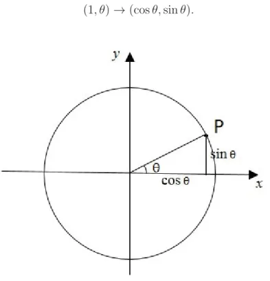
Circular data consists observations that occur around a circle and it can be represented as angles or as points on the round surface. If we create an origin and two axes and draw a circle with the origin as the center, we could use the trigonometric functions of

X andY to express the coordinates of the pointP on the circle. In this way, we could convert the polar co-ordinates into the rectangular co-ordinates easily. Letrbe the dis-tance fromP to the origin andθbe the direction, we could write down the co-ordinates of the pointP

(x=rcosθ, y =rsinθ),

in this thesis the range ofθis ﬁxed to[−π, π).

When the distancer equals to 1, the conversion between polar co-ordinates and rect-angular co-ordinates is

(1, θ)→(cosθ,sinθ).

(11)

After understanding the basic concepts of the circular data, we begin to consider some descriptive statistics of it. The ﬁrst one we want to know is the circular mean. As we know that the circular data is different from the linear data, we cannot use the normal way to calculate the mean. For example, in the ﬁgure below, suppose we have two pointsA and B, which direction are 15◦ and 345◦ respectively (suppose the North be the zero direction and clockwise as the positive sense of rotation). Here we can see, the arithmetic mean is 180◦ and it points due South whereas the true mean should be towards North.

From the example, it is obvious that the arithmetic mean is not suitable for the circular data. Besides, the sample variance, which is related with the sample mean, is also not suitable for the circular data and we should ﬁnd some alternative measures for center and dispersion if we want to deal with the circular data.

One way to calculate the circular mean is to treat the data composed of unit vectors and use the direction of their resultant vector. Letα₁, α₂,..., and α_n be a set of the cir-cular observation given in terms of angles. Recall the conversion between polar and rectangular co-ordinates, which is

(1, θ)→(x= cosθ, y= sinθ).

(12)

component-wise, and get R = ( n i=1 cosθ_i, n i=1

sinθ_i) = (COS, SIN) (1.1)

LetRrepresents the length of the resultant vectorR, where

R=||R||=√COS2+SIN2. (1.2)

Then we could get the direction ofR, which we also call the circular mean direction,θ₀.

There are two facts we know aboutθ₀is that

cosθ₀ = COS

R ,sinθ0 = SIN

R .

To ﬁndθ₀, we can do the following calculation. Since tanθ₀ = sinθ0 cosθ₀, we can get θ₀ = arctan SIN COS.

According to the property of trigonometric function, we can conclude

θ₀ = arctan SIN COS = ⎧ ⎪ ⎪ ⎪ ⎪ ⎪ ⎪ ⎪ ⎪ ⎪ ⎪ ⎪ ⎪ ⎨ ⎪ ⎪ ⎪ ⎪ ⎪ ⎪ ⎪ ⎪ ⎪ ⎪ ⎪ ⎪ ⎩ arctanSIN

COS, ifCOS >0, SIN ≥0, π

2, ifCOS = 0, SIN >0, arctanSIN

COS +π, ifCOS <0,

arctanSIN

COS + 2π, ifCOS ≥0, SIN = 0, undef ined, ifCOS =SIN = 0.

(13)

(Jammalamadaka and Sengupta, 2001)

1.3 Circular probability distribution

A circular probability distribution, literally, is a distribution with its total probability concentrated on a circumference of an unit circle. Every point on this circle has a di-rection, as we already know, the data is directional. If we measure a circular random variableθin radians, then the range of it may be taken as[0,2π)or[−π, π).

1.3.1 Generating circular distribution

To generate a circular distribution, many different models can be used. Here we give a brief introduction for a few such general methods. (Jammalamadaka and Sengupta, 2001)

Wrapped Distribution

Literally, wrapped distribution means we could wrap a linear distribution around a unit circle to conduct a circular distribution. Given a linear random variable X on the real line, we could transform it to a circular random variable by reducing its module 2π, e.g. θ = X(mod 2π). This operation is nothing but wrap the real line around the circle of unit radius, and accumulate probability over all the overlapping points x = θ, θ±2π, θ±4π, ..., so if we have the linear density functionp(x)and the corresponding circular density functionf(θ), it can be described as:

f(θ) =

∞

m=−∞

p(θ+ 2πm), −π ≤θ < π.

By using this technique, we could conduct both discrete and continuous wrapped dis-tributions.

(14)

Characterization properties

Generating a circular distribution through some characterize properties such as max-imum entropy is the most common method for normal distribution (Jammalamadaka and Sengupta, 2001 and von Mises, 1918). The circular normal distribution has the max-imum entropy property and also, its mean direction is estimated with maxmax-imum like-lihood by the direction of the resultant vector. This characterization goes back to von Mises (1918) which is why we also call circular normal distribution as the von Mises distribution.

Offset distributions

By transforming a linear random vector to its directional component, we can obtain the offset distributions (Jammalamadaka and Sengupta, 2001). We transform the bivariate random vector(X, Y)into polar co-ordinates(r, θ)and integrate overrfor a givenθ. If the joint distribution of a bivariate distribution isp(x, y), then the corresponding circular offset distributionf(x, y)is given by

g(θ) =

_∞

0

f(rcosθ, rsinθ)rdr. (1.4)

In the following part, we will describe some standard circular distributions for a general reference (see Fisher, 1995).

1.3.2 Some standard circular distribution

Uniform circular distribution

Deﬁnition 1.3.1 If the total probability is spread out uniformly on the circumference of a circle, we call it a Circular Uniform Distribution with the constant density

f(θ) = 1

2π,−π ≤θ < π.

It’s not hard to ﬁnd that, in a uniform circular distribution, all the directions have equal probability and the mean direction is undeﬁned. From the probability function we can

(15)

also write the cumulative distribution functionF(θ)as

F(θ) = θ

2π,−π ≤θ < π

Wrapped Cauchy distribution

By wrapping the Cauchy distribution on the real line we can get the wrapped Cauchy distribution. Since we know the density function of a Cauchy distribution is given by:

p(x) = (1 π)

σ

σ2+ (x−μ)2, x∈(−∞,∞). (1.5)

We could get the probability density function for a wrapped cauchy distribution:

f(θ) = 1 2π(1 + 2 ∞ k=1 ρkcosk(θ−μ)), (1.6) = ₂1 π 1−ρ2 1 +ρ2−2ρcos(θ−μ), (1.7)

whereρ=e−σ. (see Jammalamadaka and Sengupta, 2001)

This distribution is unimodal and symmetric. As ρ → 0, the distribution tends to the uniform circular distribution and asρ→ 1, the distribution goes to a point distribution with the concentrated directionμ.

Circular normal distribution

Circular normal distribution was proposed as a statistical model by von Mises (1918) and we also call it von Mises distribution. The density function of a circular random variable with this distribution is shown as below

f(θ;μ, κ) = 1

2πI_o(κ)e

κcos(θ−μ)_, _θ _∈_[₋_{π, π}₎_, _(1.8)

(16)

and order zero, and it’s given by I0(κ) = 1 2π ₂_π 0 exp(κcosθ)dθ = ∞ r=0 (κ₂)2₍1 r!) 2_. _(1.9)

Also, we could get the cumulative distribution function of the von Mises distribution based on the density function given in

F(θ) = 1 2πI₀(κ)(θI0(κ) + 2 ∞ p=1 I_p(κ) sinp(θ−μ) p ), θ∈[−π, π). (1.10)

(Jammalamadaka and Sengupta, 2001)

1.4 From parametric density estimation to nonparametric

density estimation

1.4.1 Parametric density estimation

Density estimation, basically is a method to conduct an estimator for the density func-tionf(x)from the random sample X. In statistics, it can be broadly divided into two types: parametric density estimation and nonparametric density estimation. We ﬁrstly give a brief introduction about the parametric one.

Consider a random sample X that has the probability density function f(x), and the functionf(x)gives a natural description of the distribution ofX, we know

P(a < X < b) =

_b

a

f(x)dx.

Parametric density estimation is based on a specific theoretical distribution. Suppose the distribution of the sample data is known, for example, the normal distribution with meanμand varianceσ2. We could firstly use the available data to find the estimator of

(17)

normal distribution.

Here we would like to describe one of the popular methods of parametric density esti-mation, namely, theMaximum Likelihoodmethod.

Suppose we have the data set D = {x₁, x₂, ..., x_n} corresponding to random sample

{X₁, X₂, ..., X_n}from a distribution with density function f, where (x₁, x₂, ..., x_n)are n

independent and identically distributed observations. The density functionf is from a known family of distributions. Here we supposef(x) =N(μ, σ2). Then the parameters we want to ﬁnd will beθ = (μ, σ2). (Johnson and Wichern, 2007)

Now we consider the joint density function with respect to the data setD:

f(x₁, x₂, ..., x_n|θ) =f(x₁|θ)×f(x₂|θ)× · · · ×f(x_n|θ). (1.11)

We also call the above function as likelihood function ofθ,

L(θ|x₁, ..., x_n) = n i=1

f(x_i|θ). (1.12) Then we can do some algebra to ﬁnd a value ofθ that maximizes the above function. But instead of maximizing this function, it’s usually easier to maximize the natural log-arithm of it: ln(L(θ|x₁, ..., x_n)) = ln( n i=1 p(x_i|θ)) = n i=1 lnp(x_i|θ).

We call it the log-likelihood function and one method to maximize the log-likelihood function is the standard method from Calculus.

(18)

statis-tical efﬁciency if the model is correct. Otherwise a method not dependent on a model may be more appropriate.

1.4.2 Importance of nonparametric density estimation

With the increasing application of large database and the rise of data mining, the non-parametric density estimation becomes more attractive. In a nonnon-parametric density estimation, we don’t need to know the probability density function and we just use the data itself. There are not so many restrictions such as the parametric density estimation - a parametric family of distribution or something else - we can explore the information we need just from the data set itself. It’s apparently more practical. Another attraction of nonparametric density estimation is that it’s more comprehensible for people who don’t have much statistical knowledge.

There are many kinds of nonparametric density estimation methods such as histogram estimation, nearest neighbor estimation, kernel density estimation, and so on. We will give some brief introduction for two of them in the following chapter.

(19)

Chapter 2 Nonparametric Density Estimation

2.1 General method

In this section we will give some brief introduction for some main univariate nonpara-metric density estimation.

2.1.1 Histograms

Histogram estimation is the earliest and most widely used density estimation method. Histogram is a kind of representation of the sample data. In a one-dimensional case, we divide real lines into cells that have equal size-which we also call ”bin”. Supposex₀ is the origin andhis the bandwidth, we deﬁne the bins of the histogram to be the intervals [x₀+mh, x₀+ (m+ 1)h) for any integerm, and here we choose the left of the interval is closed and the right to be an open one for the deﬁniteness. (Silverman, 1986)

Now we could write the histogram as:

ˆ

f(x) = 1

nh(number ofXi in the same bin asx).

Suppose that we have divided the real lines into bins, then the histogram estimate can be deﬁned as:

(20)

ˆ

f(x) = 1 n ×

(number ofX_i in the same bin asx)

(width of bin containingx) .

Recall that, if we want to construct a histogram, ﬁrstly we should choose a bin width and an origin. Obviously, the bin width affects much more on our estimation and it raised some problems like when we choose a big bin width and highlight the role of averaging, the potential details of the estimation may not be fully demonstrated. On the other hand, if we choose a small bin width, the random may affect too much on the histogram and we might get an irregular shape, which could lead to a not so correct conclusion.

Although histogram density estimation has some weakness, it’s still an excellent tool for data analyzing and I look forward to further study it in the future.

2.1.2 The naive estimator

As we already know, the histogram estimation has a serious problem - the bin width selection, and sometimes some extreme cases may happen. Due to the uncertainty of data, some bins might be empty while some others have more than 100 occurrences. If that so, the probability density between two adjacent bins - one has 100 occurrences and another one is empty - would vary greatly. Considering this situation, the naive estimator raised.

In this estimator, Silverman (1986) considered the deﬁnition of a probability density:

Deﬁnition 2.1.1 If the random variable X has a density f, then f(x) = lim

h→0 1

2hP(x−h < X < x+h) for any givenx.

Based on the above deﬁnition, we can choose a smallhand get the estimator by calcu-lating the proportion of all theX_i falling in the interval (x−h, x+h), then the naive

(21)

estimator is given by

ˆ

f(x) = 1

2hn(number ofX1, ..., Xnfalling in(x−h, x+h)). (2.1)

To express this estimator more transparently, Silverman (1986) deﬁned a weight func-tionwby w(x) = ⎧ ⎪ ⎨ ⎪ ⎩ 1 2, if|x|<1 0, otherwise. (2.2)

Then the naive estimator can be written as

ˆ f(x) = 1 n n i=1 1 hw( x−X_i h ). (2.3)

The generalization of the above estimator to generate weight functions gives, what is known as the kernel density estimator described below.

2.2 Kernel density estimation

2.2.1 Deﬁnition

Kernel density estimation was originally put forward by Parzen (1962) and Rosenblatt (1956), and it was popularized in many subsequent papers. The basic form of the com-mon kernel density estimator (Silverman, 1986) is described below.

Suppose (X₁, X₂, ..., X_n) is an independent and identically distributed sample of a ran-dom variable X with an unknown density functionp(x), then the kernel density estima-tor ofp(x)is given by ˆ p(x;h) = 1 nh n i=1 K(x−Xi h ), (2.4)

(22)

whereKis the kernel function, a symmetric function that integrates to 1 and its mean is 0. h is the smoothing parameter, usually called thebandwidthorwindowwidth. Gener-ally, we choose the kernel functionKto be symmetric around zero but it’s not necessary to be a positive function. Typically, the bandwidth h tends to 0 ad the sample size n

tends to inﬁnity.

There are many types of kernel functions such like:

Uniform kernel function

K(u) = 1

2I(|u| ≤1),

Triangular kernel function

K(u) = (1− |u|)I(|u| ≤1),

Quartic kernel function

K(u) = 15

16(1−u2)2I(|u| ≤1),

Gaussian kernel function

K(u) = √1

2πe

−1 2u2_.

It has been proved that the kernel density function is not the crucial part in a kernel den-sity estimator, any kernel function can guarantee the consistency of the denden-sity estima-tion (Wand and Jones, 1995). However, choosing an optimal bandwidth is a much more important problem. That is because, a big bandwidth may lead to a over-smoothed es-timator, and a small bandwidth may yield a density estimator which is spiky and very hard to explain. So we will give more details in the following part about the bandwidth selection.

2.2.2 Bandwidth selection

There are different methods for us to specify the bandwidth h, such like Rule-of-thumb, Biased cross-validation, Unbiased cross-validation and so on. Basically, they are all

(23)

based onAMISE(asymptotic mean integrated squared error). So before we get to know those methods, we would like to introduceAMISEﬁrst.

There is a vector for us to compare the estimated density function with the real one and we call itISE(integrated squared error). It’s given by:

ISE = _π −π ˆ f(x)−f(x) ₂ dx. (2.5)

By averagingISEwe could get another quantity, calledMISE(mean integrated squared error), and the asymptotic approximation for MISE is just the AMISE. The AMISE is usually derived via the Taylor’s series. Based on some certain assumptions, we have theAMISEas shown below (Tang, 2011):

AM ISE( ˆf(x;h)) = 1 nhR(K) + 1 4h4μ2(k)2R(f ). (2.6)

Hereμ2(K) = x2K(x)dx, R(K) = K2(x)dx, and f is the second derivative of the densityf.

The optimal bandwidth can be obtained by minimizing MISE, and it’s given by:

h_AMISE = ( R(K) μ2(K)2R(f)n)

1/5_. _(2.7)

However, neither theAMISEnor theh_AMISE can be used directly since there is always the unknown density function f. So now we can introduce some popular method for bandwidth selection based on these above equations.

Rule-of-thumb

Deheuvels (1977) proposed the Rule-of-thumb ﬁrstly and it was popularized by Silver-man (1986) later, and that’s why it’s also called by SilverSilver-man’s Rule-of-thumb. Based on the equation (2.7), Deheuvels proposed the kernel function K as the Gaussian dis-tribution and the standard normal disdis-tribution as the reference disdis-tribution, and the estimator ofhis given by:

ˆ

(24)

whereσ2 is the sample variance.

This method is easy to compute, however, it could also yield some problems. When the density is not close to being normal, the estimation may become inaccurate. To ﬁx that, Silverman (1986) proposed a modiﬁed estimator which can decrease this inaccu-racy:

ˆ

h_M.ROT = 1.06∗min(ˆσ, Q

1.34)n

−1/5_, _(2.9)

whereQis the interquartile range:

Q=X_[0_.₇₅_n_]−X_[0_.₂₅_n_]. (2.10) When the density is very close to the normal distribution, both estimators ˆhare good and helpful. However, if the true density is not normal distribution or we can’t deter-minate it, the second estimator gives a better result.

Unbiased cross-validation

The Unbiased cross-validation method is based on the formula of MISE:

M ISE( ˆf(x;h)) = E ( ˆf(x;h)−f(x))2dx =E ˆ f2(x;h)dx−2E ˆ f(x;h)f(x)dx+ f2(x)dx. (2.11) Chaubey et al. (2012) adapted this method Wand and Jones (1995) that we describe be-low.

Since the last term in the above function is constant, we can drive an unbiased estimator of MISE with replacing the ﬁrst two terms by its estimator.

U CV(h) = ˆ f2(x;h)dx− 2 n n i=1 ˆ f_i(X_i;h). (2.12) Noted here the second term is theleave-one-out estimatorgiven by

ˆ f_i(X_i;h) = 1 n−1 n j=i K_h(x−X_j), (2.13)

(25)

where

K_h(u) = 1 hK(

u h).

Then we can obtain an optimalhˆ_UCV by ﬁnding thehthat minimized the function (2.13).

Biased cross-validation

The biased cross-validation method was proposed by Scott and Terrell (1987). Recall the asymptotic mean squared error:

AM ISE( ˆf(x;h)) = 1 nhR(K) + 1 4h4μ2(k)2R(f ). (2.14)

To get the estimator ofh, they used the estimated function ofR(f)instead of a reference distribution, ˆ R(f) = 1 n2 i=j (K_h∗K_h)(X_i−X_j). (2.15) Then it leads to the score function:

BCV(h) = R(K) nh +h 4μ22(K) 4n2 i=j (K_h∗K_h)(X_i−X_j). (2.16) Scott and Terrell (1987) proposed to use the optimal bandwidthˆh_BCV which could min-imize the function above.

Conclusion

After we introduced some widely used bandwidth selection methods, an important question must be asked by ourselves: which method is the most efficient one? It’s really difficult to define which one is ”the best”, since it all depends on the situation. When we analyze a real data set, the best way for us to select the ”best” bandwidth is to apply dif-ferent bandwidth selectors to our data and try to compare all the possible bandwidths, and then we could find out the most suitable one for our data.

(26)

2.3 Asymmetric density estimation

Since the standard symmetric ﬁxed kernels are not appropriate for some density func-tions with bounded support, asymmetric kernels presented. Kernel density estima-tor with asymmetric kernels such as gamma kernels have been proposed to solve the boundary consistency problem. For example, Chen (2000) used Gamma kernels and Scaillet (2004) used inverse Gaussian (IG) and reciprocal inverse Gaussian (RIG). To fo-cus on the case of non-negative data, Chaubey et al. (2012) proposed an estimator which is based on the generalization of Hille’s smoothing lemma (Feller, 1965).

Lemma 2.3.1 Letube any bounded and continuous function andG_x,n, n=1,2,. . . be a family of distributions with meanμ_n(x)and varianceh2_n(x)such thatμ_n(x)→xandh_n(x)→0. Then

ˆ

u(x) =

_∞

−∞

u(t)dG_x,n(t)→u(x). (2.17)

The convergence is uniform in every subinterval in whichh_n(x) → 0uniformly and uis uni-formly continuous.

According to this lemma, the smooth estimator of an empirical distribution function

F(x)could be obtained easily by replaceu(x)withF_n(x)

ˆ

F_n(x) =

_∞

−∞

F_n(t)dG_x,n(t). (2.18)

To obtain more details about Fˆ_n(x), Chaubey et al. (2012) considered the following theorem.

Theorem 2.3.1 Leth_n(x)to be the variance ofG₍x, n)as in Lemma , and suppose thath_n(x)→

0asn →0for every ﬁxedx. Then we have

sup

x |

F_n(x)−F(x)| −→a.s. 0 (2.19)

(27)

A restricted condition onG_x,n(X_i)can be seen easily if we change the form ofF_n(x)to:

F_n(x) = 1− 1

nGx,n(Xi). (2.20)

ForF_n(x)to be a proper distribution function,G_x,n must be a decreasing function ofx.

Based on that, we can get the smooth estimator of the density function given by:

ˆ f_n(x) = dFn(x) dx =−1 n n i=1 d dxGx,n(Xi). (2.21)

2.4 Bernstein polynomial estimation

The empirical distribution function is known to have good properties when we use it to estimate distribution function. However, since it’s not a continuous function, it may not be appropriate to use it to estimate a continuous distribution function. Babu, Canty and Chaubey (2002) considered the application of Bernstein polynomials to approximate a bounded and continuous function, and they proved that with a continuous approxima-tion of the empirical distribuapproxima-tion funcapproxima-tion, the Bernstein polynomials could be naturally adapted to smooth an estimated distribution function that concentrated on the interval [0,1].

We ﬁrstly have a look at the deﬁnition of the empirical distribution function:

F_n(x) = 1 n n i=1 I{X_i ≤x}. (2.22)

The above function is appropriate when the support of distribution isR+. If we have the support of F in the interval [a,b], wherea ≤ b, it would be better to transform the variable X to Y with support [0,1]. This transformation could be done by Y = X_b₋−_aa. Based on that, Babu, Canty and Chaubey (2002) introduced the following theorem to adapt Bernstein polynomials to estimation.

(28)

Theorem 2.4.1 (Feller, 1965) If u(x) is a bounded and continuous function on the interval [0,1], then asm→ ∞ u∗_m(x) = m k=0 u(k/m)b_k(m, x)→u(x) (2.23)

uniformly forx∈[0,1], where b_k(m, x) = m k xk(1−x)m−k, k = 0, . . . , m. (2.24)

With the theorem given below, Babu, Canty and Chaubey (2002) consideredF with sup-port [0,1], and motivated the smooth estimatorFbased on Bernstein polynomial, which is given by: ˆ F_n,m(x) = m k=0 F_n(k m)bk(m, x), x∈[0,1] (2.25)

Noted here this estimator is based on the empirical distribution functionF_n:

F_n(x) = n−1 n

i=1

I{X_i ≤x}. (2.26)

To prove that Fˆ_n,m is a proper distribution function and it has derivative, consider an alternative form of the function in (2.25).

ˆ F_n,m(x) = m k=0 f_n(k m)Bk(m, x), (2.27) where f_n(0) = 0, f_n(k m) =Fn( k m)−Fn( k−1 m ), k = 1, . . . , m (2.28) and

(29)

B_k(m, x) = m j=k b_k(m, x) =m m−1 k−1 x 0 tk−1(1−t)m−kdt. (2.29)

The above equation is given by the deﬁnition of the cumulative distribution function of a binomial distribution. Sinceb_k(m, x)is just the form of the probability mass function of a binomial distribution with parameters m, k, x, B_k(m, x) =

m

j=k

b_k(m, x) will be the probability mass function of this given binomial distribution. From the deﬁnition we can get the equation ofB_k(m, x).

Noted hereFˆ_n,m is a polynomial in terms ofxso it’s continuous and has all the deriva-tives, and0≤Fˆ_n,m ≤1forxin interval[0,1]. Based on the equations in (2.28) and (2.29), we can see that f_n(_mk)is a non-negative polynomial and B_k(m, x)is non-decreasing in

x. Thus, we knowFˆ_n,m is non-decreasing also.

Upon taking the derivative of Fˆ_n,m, we can get the density estimator off as proposed in Babu, Canty and Chaubey (2002):

ˆ f_n,m(x) = m k=1 f_n(k m) d dxBk(m, x) =m m−1 k=0 f_n(k+ 1 m )bk(m−1, x) =m m−1 k=0 (F_n(k+ 1 m )−Fn( k m)bk(m−1, x)). (2.30)

(30)

Chapter 3 Transformation Based Nonparametric

Density Estimators

3.1 General method

Recall the kernel density estimator and if we consider it for circular data, we can assume a continuous circular density functionf(θ), where θ ∈ [−π, π), f(θ) ≥ 0for θ ∈ R and

_π

−πf(θ)dθ = 1.

For a random sample that satisﬁes the above density function, i.e. (θ₁, ..., θ_n), we can write the kernel density estimator as follows:

ˆ f(θ;h) = 1 nh n i=1 K(θ−θi h ). (3.1)

To obtain this density estimator, Fisher (1989) used the quartic kernel function to adapt the linear kernel density estimator and deﬁned the kernel function:

K(θ) = ⎧ ⎪ ⎨ ⎪ ⎩ 0.9375(1−θ2), ifθ∈[−1,1] 0, otherwise. (3.2)

(31)

to ensure that K(θ)dθ = 1and K(θ)is a density function. It’s indeed one method to do the transformation but here is one obvious problem-the estimator is not periodic. To ﬁx this, Fisher (1995) suggested to perform the smoothing by replicating the data to 3 to 4 circles and consider only one interval,[−π, π).

3.2 Transformation based kernel density estimator

Since the major different between circular data and linear data is the type of data, we may adapt the linear density estimator to the circular density estimator by transform-ing the data interval. In this section we will focus on kernel density estimator and try to transform the data on[−π, π)to(−∞,∞). (Chaubey, 2017)

Let f(θ) be the density function of the circular data and p(x) be the density function of the linear data. Suppose x =t(θ)is the one-to-one transform function t : (−π, π) →

(−∞,∞), e.g. t(θ) = tan(θ₂).

Using the transformation and the fact that

f(θ) =p(t(θ))|dt(θ) dθ |,

and recall the kernel density estimator ofx:

ˆ p_K(x;h) = 1 nh n i=1 K(x−xi h ) = 1 nhK( x−tan(θ_i/2) h ), (3.3)

then this transformation could be done by the following steps:

ˆ

f_K(θ;h) = p(t(θ);h)|d(t(θ))

(32)

where t(θ) = tan(θ 2) = sinθ 1 + cosθ, and d(t(θ)) d(θ) = ( sinθ 1 + cosθ)

= cosθ(1 + cos_{(1 + cos}θ) + sin2θ

θ)2 = 1 1 + cosθ, then ˆ f_K(θ;h) = 1 1 + cos(θ)pˆ( sinθ 1 + cosθ;h) (3.5)

is the estimator for the circular density function.

3.3 Transformation based Bernstein polynomial density

estimator

Another transformation between circular density estimator and linear density estima-tor can be done based on Bernstein polynomials (Chaubey, 2017). We introduced the Bernstein polynomials estimator (Babu, Canty and Chaubey, 2002) in chapter 2, and to differentiate the circular density function from the linear one, we denote the linear Bern-stein polynomial density estimator bypˆ(x;m), and it’s given by

ˆ p_B(x;m) =m m k=1 F_n(k m)bk(x;m−k+ 1), x∈[0,1], (3.6)

(33)

Chaubey (2017) considered the following transformation: t(θ) = 1 2+ 1 πtan −1₍_c_tan(θ 2)), (3.7)

wherecis a positive number.

With this function, we could convert the interval of θ - which is [−π, π) to [0,1), and it’s also a one-to-one transformation for all c >0. An important thing is that the trans-form functiont(θ)is periodic.

Now the transformed estimator off(x)can be obtained and it’s given by

ˆ

f_B(θ;m) = 1

2πpˆB(t(θ);m)

c(1 + tan2(θ₂))

(34)

Chapter 4 A Simulation Study

4.1 Introduction

In order to compare the two estimators we discussed in Chapter 3, I would like to use simulation method in this chapter. Concerning the data we would like to use is circular data, I’d like to introduce ISE and MSE as the reference for comparing them.

For ISE, integrated squared error, the function is given by:

ISE =

_∞

−∞( ˆ

f(x)−f(x))2dx. (4.1)

From the function above, we can see that the value of ISE is the square of the distance between the estimated density and the simulated density. We can simplify the function as:(Chaubey et al., 2012) ISE = _∞ −∞( ˆ f(x)−f(x))2dx (4.2) = _∞ −∞ ˆ f2(x)dx−2 _∞ −∞ ˆ f(x)f(x)dx+ _∞ −∞ f2(x)dx. (4.3)

The above function motivated a method to smooth the parameter, which is called unbi-ased cross validation. Since the third term in the functionISE is constant, and we can

(35)

estimate the second term by theleave−one−outestimator 2_nfˆ_n(X_i;ω_i),

where ω_i = {X₁, ..., X_i₋₁, X_i₊₁, ...X_n}. The estimated ISE with cross-validation in our case is given by:

CV_ISE = _π −π ˆ f2(x)dx− 2 n n i=1 ˆ f_n(X_i;ω_i). (4.4) With this unbiased estimator ofISE, we could obtain the optimal h in the kernel den-sity estimator andmin the Bernstein polynomial density estimator by minimizing the

ISE.CV function. To makes it more clearly, I will check the mean, median and standard deviation of ISE and M SE for these two estimators based on different distributions and different sample sizes.

Before we start the simulation, it’s better to look at the range of bandwidth in the kernel estimator ﬁrstly. Here we use the Gaussian kernel function as the kernel functionK and it’s given by:

K(u) = √1

2πe

−1

2u2_. _(4.5)

When we plug the kernel function into the kernel density estimator for circular data,

ˆ

f_K(θ;h) = 1

1 + cos(θ)pˆ(

sinθ

1 + cosθ;h), (4.6)

and here the estimated density function for linear data is given by:

ˆ p(x;h) = 1 nh n i=1 K(x−xi h ), (4.7)

we can see that the density function is nothing but the mean of the following function:

k(θ, h) = 1

h(1 + cos(θ))K(

tan(θ/2)−tan(θ_i/2)

h ). (4.8)

Noted here we want the kernel estimated density function to be symmetric around zero and it also has the maximum value in zero, so we have to ensure that when x−xi

h equals

to0, the derivative of functionkˆis also0. To make it more convenient for us to study, we useθto replacetan(θ/2)−tan(θ_i/2)in equation 4.8 and took a look at the plot of the

(36)

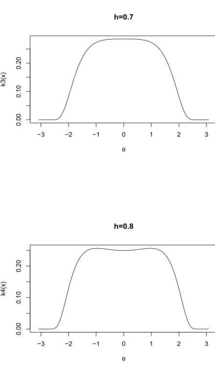
following function: ˆ k(θ, h) = 1 h√2π(1 + cosθ)exp −₂1 h2( sinθ 1 + cosθ) 2_. _(4.9) −3 −2 −1 0 1 2 3 0.0 0.1 0.2 0.3 0.4 h=0.5 θ k1(x) −3 −2 −1 0 1 2 3 0.00 0.10 0.20 0.30 h=0.6 θ k2(x)

(37)

−3 −2 −1 0 1 2 3 0.00 0.10 0.20 h=0.7 θ k3(x) −3 −2 −1 0 1 2 3 0.00 0.10 0.20 h=0.8 θ k4(x)

(38)

Whenh= 0.5, the given function is definitely symmetric around zero and its maximum value also appears at zero. With the value of h becomes larger, the upper part gets more flatter. For h = 0.7, the peak almost disappear and it’s very flat. Even more, when

h= 0.8, the upper part becomes hollow and two peak shows up. Since the special con-dition we want to have for functionkˆ(θ, h), we restrict hto be smaller than or equal to 0.6 in this thesis.

In this simulation we considered 3 models in total: wrapped Cauchy distribution with (σ=1, μ=0), von Mises distribution with (κ=1, μ=0), and a mixture distribution of 40% von Mises distribution with (κ=1, μ=0) and 60% Wrapped Cauchy distribution with (σ=1,μ=0). The domain for each model is in[−π, π).

4.2 Global comparison

Here are the results of our global comparison for these two estimators. Noted here the function we used to calculate ISE is given by:

ISE =

_π

−π( ˆ

f(x)−f(x))2dx, (4.10)

and the parameter h is obtained by unbiased cross validation method we mentioned before.

(39)

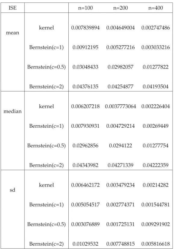
ISE n=100 n=200 n=400 mean kernel 0.007839894 0.004649004 0.002747486 Bernstein(c=1) 0.00912195 0.005277216 0.003033216 Bernstein(c=0.5) 0.03048433 0.02982057 0.01277822 Bernstein(c=2) 0.04376135 0.04254877 0.04193504 median kernel 0.006207218 0.0037773064 0.002226404 Bernstein(c=1) 0.007930931 0.004729214 0.00269449 Bernstein(c=0.5) 0.02962856 0.0294122 0.01277754 Bernstein(c=2) 0.04343982 0.04271339 0.04222359 sd kernel 0.006462172 0.003479234 0.00214282 Bernstein(c=1) 0.005054517 0.002774371 0.001544781 Bernstein(c=0.5) 0.003076889 0.001725131 0.009291902 Bernstein(c=2) 0.01029532 0.007748815 0.005816618

Table 4.1: Transformation based on different estimators with wrapped Cauchy distribu-tion (σ=1,μ=0)

If we focus on Bernstein polynomial density estimator only, we notice that as the value ofc goes greater, the average value of ISE is also getting greater and the accuracy of estimation is declining. At the same time, when we decrease the value ofc, the

(40)

aver-age value ofISEalso gets greater, which gives us the result thatc = 1gives us a better estimation than othercvalues. So we will only compare kernel density estimator with Bernstein polynomial density estimator withc= 1

When we compare the kernel density estimator with the Bernstein polynomial density estimator, we found that the kernel density estimator performs a little better than Bern-stein polynomial density estimator when sample size n=100. As the sample size goes greater, the difference between their ISE values becomes smaller and smaller. When sample sizenis 400, these two estimators’ISEvalues are very close.

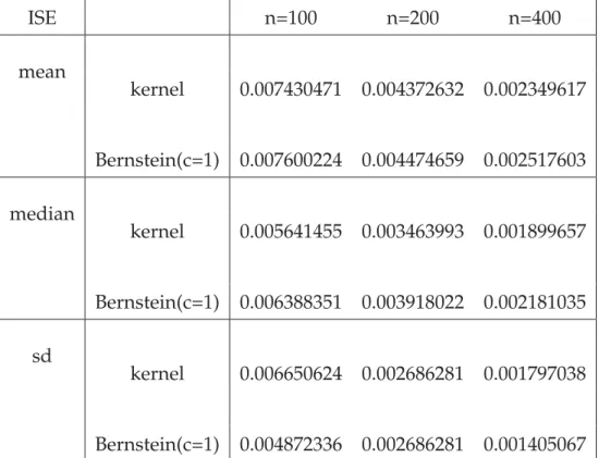
ISE n=100 n=200 n=400 mean kernel 0.007430471 0.004372632 0.002349617 Bernstein(c=1) 0.007600224 0.004474659 0.002517603 median kernel 0.005641455 0.003463993 0.001899657 Bernstein(c=1) 0.006388351 0.003918022 0.002181035 sd kernel 0.006650624 0.002686281 0.001797038 Bernstein(c=1) 0.004872336 0.002686281 0.001405067

Table 4.2: Transformation based on different estimators with von Mises distribution (κ=1,μ=0)

In the second model, the performance of kernel density estimator still looks like very similar with Bernstein polynomial density estimator since theirISEvalues are very close for all three sample sizes.

(41)

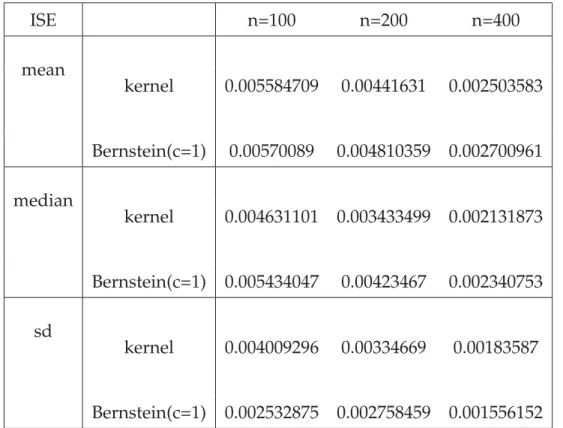
ISE n=100 n=200 n=400 mean kernel 0.005584709 0.00441631 0.002503583 Bernstein(c=1) 0.00570089 0.004810359 0.002700961 median kernel 0.004631101 0.003433499 0.002131873 Bernstein(c=1) 0.005434047 0.00423467 0.002340753 sd kernel 0.004009296 0.00334669 0.00183587 Bernstein(c=1) 0.002532875 0.002758459 0.001556152

Table 4.3: Transformation based on different estimators with Mixture distribution

In the third model, we considered a mixture distribution of 40% von Mises distribution and 60% wrapped Cauchy distribution. The result shows that kernel density estimator still performs much similar as Bernstein polynomial density estimator since their ISE

values are very close.

We cannot decide which estimator is better only depend on their ISE values, and we would like to continue our local comparison based onMSE.

(42)

4.3 Local comparison

In this section we will focus on the factorMSE, mean square error, which deﬁned as

M SE( ˆf(θ)) = 1 NE ( ˆf(θ)−f(θ)) 2 _(4.11) = ( ˆf(θ)−f(θ))2f(θ)dθ.

Instead of computing theMSEdirectly, we would like to choose the estimator of it:

ˆ M SE = 1 N N i=1 ( ˆf_i(θ)−f(θ))2, (4.12)

whereN is the replication number. (Allen, 1971)

This M SEˆ is easier for us to compute, and it could also tell us the estimate ability of these two estimators.

We’d like to express the performance ofMSEin form of graphs, and consider different sample size we have in each distribution, there will be 9 cases in total: wrapped Cauchy distribution with parameters (σ=1, μ=0) and sample size n=(100, 200, 400) separately, von Mises distribution with parameters (κ=1, μ=0) and sample size n=(100, 200, 400) separately , mixture distribution of 40% von Mises distribution with parameter (κ=1,

μ=0) and 60% wrapped Cauchy distribution with parameter (σ=1,μ=0) and sample size

n=(100, 200, 400) separately.

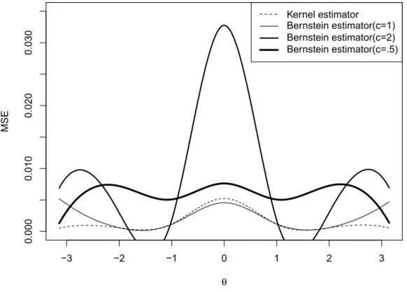
In the ﬁrst case we compared kernel density estimator and Bernstein polynomial den-sity estimator with c= (1,2,0.5), and the effect of increasing or decreasing the value of

cis exactly the same as what we found in global comparison. c = 1 results in a better estimation in our case. So we will only compare kernel density estimator with Bernstein polynomial density estimator withc= 1in the left 5 cases.

(43)

−3 −2 −1 0 1 2 3 0.000 0.010 0.020 0.030 θ MSE Kernel estimator Bernstein estimator(c=1) Bernstein estimator(c=2) Bernstein estimator(c=.5)

(44)

−3 −2 −1 0 1 2 3 0.000 0.001 0.002 0.003 0.004 θ MSE Kernel estimator Bernstein estimator(c=1)

(45)

(46)

(47)

(48)

(49)

(50)

(51)

(52)

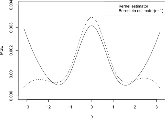
4.4 Conclusion and further research

4.4.1 Conclusion

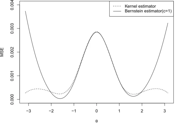
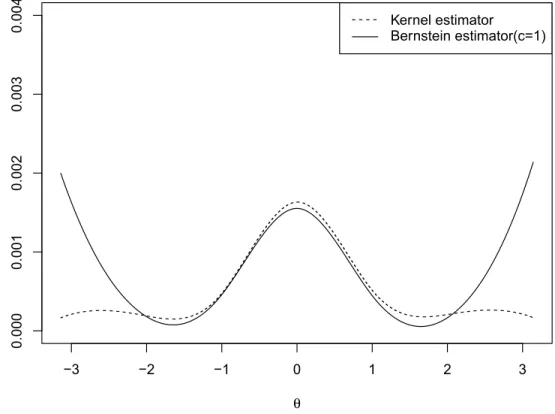
In the ﬁrst case (n = 100) of the ﬁrst distribution (Figure 4.2), if we focus on the tails, we can see that kernel estimator performs better than Bernstein estimator, and comparing different values ofc,c= 0.5gives a better result thanc= 1andc= 2. However, in the central part, Bernstein polynomial estimator withc= 1performs pretty much similar to the kernel density estimator, and as the value ofcbecomes greater (c=2) smaller (c=.5), the value of MSE also increases conspicuously. Further looking at the result with dif-ferent sample sizes, we see that these two estimators are quite similar when estimating the central part, and for the tails, kernel density estimator performs much better than Bernstein polynomial estimator. So in general we can say that kernel density estimator is more accurate than Bernstein polynomial estimator for the wrapped Cauchy distribu-tion. However, investigation by considering other circular probability density functions for simulation may be desired.

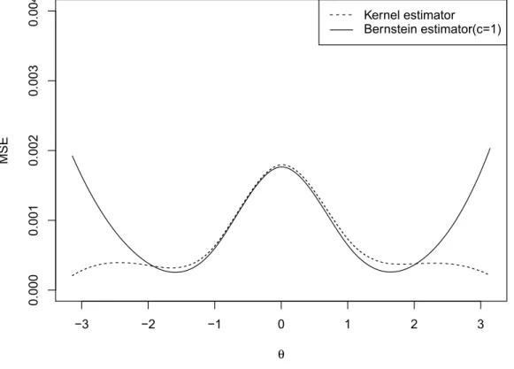
Figure 4.5, 4.6 and 4.7 give the results based on von Mises distribution. In this case kernel estimator still performs better than Bernstein estimator when we estimate the tails. However, for estimating the central part, Bernstein estimator performs a little bit better than kernel estimator when the sample size is not big enough. As the sample size goes bigger, the performances of these two estimator becomes very similar.

For the third distribution (See Figure 4.8, 4.9 and 4.10), the result also shows that kernel estimator has a stronger estimation ability than Bernstein estimator. In general, these two transformations are very comparable when we estimate the central part for all dis-tributions, however, the kernel transformation are much more efﬁcient than Bernstein transformation when it comes to the tail.

To sum it up, for all distributions we mentioned in this chapter, the performances of these two estimators are very similar when estimating the central part and the kernel estimator is more efﬁcient than the Bernstein estimator with the tail part. In general

(53)

we can say, the kernel density estimator is better than Bernstein polynomial density estimator.

4.4.2 Further research

Since we just compared two estimators based on three models, it’s conspicuous that kernel density estimator has a stronger ability to alleviate the boundary problem than Bernstein polynomial density estimator in these models. However, we may need to do more about the boundary problems in the transformed Bernstein polynomial density estimator. On the other hand, we just used three different sample size to do the research and small sample size may cause many problems, so more tests with larger sample size may be needed in the further research.

Another important line of investigation would be to consider other circular probability distribution for simulation which are not necessarily symmetric. One way to generate such distribution would be to consider mixture distribution such as the one considered in this thesis, but with different mean directions.

Also for a deﬁnitive treatment for the choice of c could be to analyze the asymptotic nature of theMISE; the leading term may cast some light on its optimal choice.

(54)

APPENDIX: R codes for computing ISE

and MSE for transformed kernel density

estimator (Based on Wrapped Cauchy

distribution (

σ

_=1,

μ

₌₀₎₎

## Global E r r o r : ISE ## Kernel e s t i m a t o r

##Wrapped Cauchy D i s t r i b u t i o n

##p . d . f o f wrapped cauchy d i s t r i b u t i o n with mu=o , rho=exp (−1) WCauchyf= f u n c t i o n ( t h e t a ){

( 1 / ( 2∗p i ) )∗( ( 1−( exp (−1 ) ) ˆ 2 ) / ( 1 + ( exp (−1))ˆ2−2∗exp (−1)∗cos ( t h e t a ) ) )

} ## f h a t f u n c t i o n f h a t . k e r n e l<−f u n c t i o n ( t h e t a , t h e t a s , h ){ dcnorm<−f u n c t i o n ( t h e t a , h ){ ( 1 / ( ( 2∗p i ) ˆ 0 . 5∗h∗(1+ cos ( t h e t a ) ) ) )∗exp (−0 . 5∗( s i n ( t h e t a )/ ( h∗(1+ cos ( t h e t a ) ) ) ) ˆ 2 ) } xs<−tan ( t h e t a s /2) mean ( dcnorm ( t h e t a−t h e t a s , h=h ) )

(55)

} #CV. ISE f u n c t i o n CVISE . k e r n e l<−f u n c t i o n ( h , t h e t a s ){ n<−l e n g t h ( t h e t a s ) FT . I n t<−f u n c t i o n ( t h e t a , t h e t a s = t h e t a s , h=h ) {( f h a t . k e r n e l ( t h e t a , t h e t a s , h ) ) ˆ 2} FT<−V e c t o r i z e ( FT . I n t , ” t h e t a ” ) f i r s t . termK<−i n t e g r a t e ( FT,−pi , pi , t h e t a s = t h e t a s , h=h ) $value # second term ST<−0 f o r ( i i n 1 : n ){ ST=ST+ f h a t . k e r n e l ( t h e t a s [ i ] , t h e t a s = t h e t a s [−i ] , h=h ) } second . termK<−2∗ST/n

cv<−f i r s t . termK−second . termK r e t u r n ( cv )

}

## Minimize CV. ISE t o f i n d h

h . cv=as . numeric ( o p t i m i s e ( CVISE . k e r n e l , i n t e r v a l =c ( 0 , 0 . 6 ) , t h e t a s = t h e t a s ) [ 1 ] ) ## D e f i n i t i o n o f ISE func . i n t e g r a n d = f u n c t i o n ( t h e t a , t h e t a s , h ){ ( f h a t . k e r n e l ( t h e t a , t h e t a s , h)−WCauchyf ( t h e t a ) ) ˆ 2 } ISE . k e r n e l = r e p l i c a t e ( 1 0 0 0 ,{

(56)

h . cv=as . numeric ( o p t i m i s e ( CVISE . k e r n e l , i n t e r v a l =c ( 0 , 0 . 6 ) , t h e t a s = t h e t a s ) [ 1 ] )

i n t e g r a t e ( func . integrand ,−p i + 0 . 1 , pi , t h e t a s = t h e t a s , h=h . cv ) $value

}) mean ( ISE . k e r n e l ) median ( ISE . k e r n e l ) sd ( ISE . k e r n e l ) ## L o c a l E r r o r : MSE ## Kernel e s t i m a t o r ##Wrapped Cauchy D i s t r i b u t i o n

##p . d . f o f wrapped cauchy d i s t r i b u t i o n with mu=o , rho=exp (−1) WCauchyf= f u n c t i o n ( t h e t a ){

( 1 / ( 2∗p i ) )∗( ( 1−( exp (−1 ) ) ˆ 2 ) / ( 1 + ( exp (−1))ˆ2−2∗exp (−1)∗cos ( t h e t a ) ) )

} #MSE d e f i n i t i o n f o r k e r n e l t r a n s f o r m a t i o n mse . k e r n e l . wc= f u n c t i o n ( t h e t a , t h e t a s , h ){ ( f h a t . k e r n e l ( t h e t a , t h e t a s , h)−WCauchyf ( t h e t a ) ) ˆ 2 } t h e t a . mse=seq (−pi , pi , l e n g t h . out = 7 ) MSE . wc= r e p l i c a t e ( 1 0 0 0 ,{ t h e t a s =rwrpcauchy ( 1 0 0 , l o c a t i o n = pi , rho=exp (−1))−p i

h . cv=as . numeric ( o p t i m i s e ( CVISE . k e r n e l , i n t e r v a l =c ( 0 , 0 . 6 ) , t h e t a s = t h e t a s ) [ 1 ] )

MSEmatrixy=sapply ( t h e t a . mse , mse . k e r n e l . wc , t h e t a s = t h e t a s , h=h . cv ) MSEmatrixy

(57)

}) KernelMSE1=rowMeans (MSE . wc ) #MSE P l o t f o r k e r n e l e s t i m a t o r sp1= s p l i n e ( t h e t a . mse , KernelMSE1 , n =1000) p l o t ( sp1 , ylim=c ( 0 , 0 . 0 3 5 ) , x l a b = e x p r e s s i o n ( t h e t a ) , y l a b =”MSE” , type =” s ” , l t y =2)

(58)

(59)

REFERENCES

Allen, D. M. (1971). Mean square error of prediction as a criterion for selecting variables.

Technometrics,13(3):469–475

Babu, G. J., Canty, A. J., and Chaubey, Y. P. (2002). Application of bernstein polynomi-als for smooth estimation of a distribution and density function. Journal of Statistical Planning and Inference,105(2):377–392.

Chaubey, Y. P., Li, J., Sen, A., and Sen, P. K. (2012). A new smooth density estimator for non-negative random variables. Journal of the Indian Statistical Association,50:83–104 Chaubey, Y. P. (2017). On smooth density estimation for circular data. Invited Paper,

Presented at 61st World Statistics Congress, Marrakech July 16–21, 2017.

Chaubey, Y. P. (2018). Smooth kernel estimation of a circular density function: A connec-tion to orthogonal polynomials on the unit circle. Journal of Probability and Statistics,

2018, Article ID 5372803.

Chen, S. X. (2000). Probability density function estimation using gamma kernels.Annals of the Institute of Statistical Mathematics,52(3):471–480.

Deheuvels, P. (1977). Estimation non paramétrique de la densité par histogrammes généralisés. Rev. Statist. Appl,25(3):5–42.

Feller, W. (1965). An Introduction to Probability Theory and its Applications, Vol. 1, Wiley: New York.

Fisher, N. I. (1989). Smoothing a sample of circular data. Journal of structural geology,

(60)

Fisher, N. I. (1995). Statistical Analysis of Circular Data. Cambridge University Press, London.

Jammalamadaka, S. R. and Sengupta, A. (2001). Topics in Circular Statistics. World Sci-entiﬁc, Singapore.

Johnson, R. A. and Wichern, D. W. (2007). Applied Multivariate Statistical Analysis. Pear-son Education.

Parzen, E. (1962). On estimation of a probability density function and mode. The Annals of Mathematical Statistics,33(3):1065–1076.

Rosenblatt, M. (1956). Remarks on some nonparametric estimates of a density function.

The Annals of Mathematical Statistics,27(3):832–837.

Scaillet, O. (2004). Density estimation using inverse and reciprocal inverse gaussian kernels. Nonparametric Statistics,16(1-2):217–226.

Scott, D. W. and Terrell, G. R. (1987). Biased and unbiased cross-validation in density estimation. Journal of the American Statistical Association,82(400):1131–1146.

Silverman, B. W. (1986). Density Estimation for Statistics and Data Analysis. Chapman and Hall Ltd., London.

Tang, M. (2011). A Comparison of Two Nonparametric Density Estimators in the Context of Actuarial Loss Model. PhD Thesis, Concordia University.

von Mises, R. (1918). Uber die’ganzzahligkeit’der atomgewicht und verwandte fragen.

Phys. Z.,19:490–500.

On Transformation Based Circular Density Estimators