Fast Traffic Sign Recognition Using
Color Segmentation and Deep
Convolutional Networks
Ali Youssef, Dario Albani, Daniele Nardi, and Domenico D. Bloisi
Department of Computer, Control, and Management Engineering, Sapienza University of Rome
via Ariosto 25 - 00185 Rome (Italy)
<lastname>@diag.uniroma1.it
Abstract. The use of Computer Vision techniques for the automatic recognition of road signs is fundamental for the development of intelli-gent vehicles and advanced driver assistance systems. In this paper, we describe a procedure based on color segmentation, Histogram of Ori-ented Gradients (HOG), and Convolutional Neural Networks (CNN) for detecting and classifying road signs. Detection is speeded up by a pre-processing step to reduce the search space, while classification is carried out by using a Deep Learning technique. A quantitative evaluation of the proposed approach has been conducted on the well-known German Traf-fic Sign data set and on the novel Data set of Italian TrafTraf-fic Signs (DITS), which is publicly available and contains challenging sequences captured in adverse weather conditions and in an urban scenario at night-time. Experimental results demonstrate the effectiveness of the proposed ap-proach in terms of both classification accuracy and computational speed.
1
INTRODUCTION
The increasing interest towards autonomous vehicles and advanced driver assis-tance systems is demonstrated by the prototypes developed by Google, Volvo, Tesla, and other manufacturers. In this paper, we focus on the use of visual information for traffic sign recognition, which is fundamental for achieving au-tonomous driving in real world applications.
In recent years, many methods for traffic sign detection (TSD) and recog-nition (TSR) based on Computer Vision techniques have been proposed. Since road signs have bright fixed colors (for aiding human detection), some approaches are based on color segmentation to locate the signs in the input images. Sliding windows approaches have also been proposed, relying mostly on the use of His-togram of Oriented Gradients (HOG), Integral Channel Features (ICF) and its modifications [11] to extract discriminative visual features from the images. Our method aims at combining the speed of the color segmentation techniques with the accuracy of sliding windows approaches, in particular HOG.
Color information from high resolution images in input is used to select a set of regions of interest (ROIs), thus reducing the search space. Then, visual features are extracted from each ROI and compared with a Support Vector Machine (SVM) model for detecting road signs. Finally, a Convolutional Neural Network (CNN) is used for the recognition of the traffic signs. Different architectures for the network are proposed, starting from the ones presented in [13] and [9]. For the implementation of the net, we rely on TensorFlow1, a recent open source
framework released by Google.
Quantitative experimental results have been carried out on the publicly avail-able German Traffic Sign Data set (GTSRB) in order to allow a comparison with other approaches. Moreover, we have created a novel publicly available data set, called the Data set of Italian Traffic Signs (DITS), containing Italian traffic signs captured in challenging conditions (i.e., nigh-time, fog, and complex urban sce-narios). The results demonstrate that our method achieves good results in terms of accuracy, requiring only 200 milliseconds per image for processing HD data.
The contributions of this paper are threefold:(i) A new approach for speed-ing up the traffic sign detection process is proposed. (ii) A complete pipeline, including sign detection and recognition, is described. (iii) A novel challenging data set, called DITS, has been created and made publicly available.
The rest of the paper is organized as follows. Section 2 provides a brief overview of the state-of-the-art methods for traffic signs detection and classifica-tion in single images. Our method is presented in Secclassifica-tion 3. The newly created DITS data set is described in Section 4, while the experimental results, carried out both on DITS and on GTSRB, are presented in Section 5. Finally, conclu-sions are drawn in Section 6.
2
RELATED WORK
The problem of automatically recognizing road signals from cameras mounted on cars is gaining more and more interest with the advent of advanced driver assisted systems to help the driver in avoiding potentially dangerous situations. According to the different tasks in image recognition pointed out by Perona in [12], the problem of recognizing traffic signs in single images can be divided into two sub-problems, namely detection and classification.
Detection. Given an image, the goal is to decide if a sign is located somewhere in the scene and to provide position information about it, i.e., the image patch containing the sign. Detection can be carried out by analysing images from single or multiple views. Although traditional systems count on the single view approach (e.g., [1]), today’s cars are often equipped with multiple cameras, thus multi-view data are often available. Since existing work on multi-view recognition consists of single-view sign detection followed by a multi-view fusing step [15], we will discuss here single-view approaches with the consideration that they can be conveniently adapted when multiple views are available.
1
Mathias et al. published a recent review on the current state-of-the-art for single-view methods [10]. Top performance can be reached by using approaches designed for pedestrian (i.e., HOG features) and face (i.e., Haar-like features) detection. Another widely used technique in traffic sign detection, which has been originally developed for pedestrian detection, is based on Integral Channel Features [4]: multiple registered image channels are computed by using linear and non-linear transformations of the input image. Features (e.g., Haar-like wavelets and local histograms) are extracted from each channel along with integral images. Variants of the Integral Channel Feature detector (e.g., [2,5]) have demonstrated to reach high speed (i.e., 50 frames per second) maintaining accurate detection. Classification. Given the image patch extracted in the detection phase, the classification problem consists in deciding if it contains a sign among the possible sign categories. A common pipeline for classification [10] is made of three stages: (i) Feature Extraction, (ii) Dimensionality Reduction, and (iii) Labeling. Ex-tracting visual features from the image at hand is the first step for classification. Since traffic signs are designed for colour-blind people, visual features like shape and inner pattern are more descriptive than color attributes. This is demon-strated by Mathias et al. [10] in their experiments, where no gain is obtained by using color-dependent features for classification in place of grayscale features. Dimensionality reduction plays an important role on classification. Timofte et al. in [16] present a technique called Locality Preserving Projections (LPP) that represent an alternative to the classical Principal Component Analysis (PCA). A LPP variant is the Iterative Nearest Neighbours based Linear Projection (INNLP) presented in [17]. It uses iterative nearest neighbours instead of sparse representations in the graph construction.
The labeling step is the last phase in the pipeline. The competition2 on
the German Traffic Sign Recognition Benchmark (GTSRB) has allowed to test and compare different solutions for road sign classification. Among those, Deep Learning based methods obtained great results. In particular, Ciresan et al. [3] won the final phase of the competition using a GPU implementation of a Deep Neural Network (DNN), further improved in a Multi-Column DNN that makes the system robust to variations in contrast and illumination. Sermanet et al. [13] use a Multi-Scale Convolutional Neural Network, obtaining results above the average human performance. Extreme Learning Machine classifier fed with CNN features is proposed by Zeng et al. in [20], obtaining competitive results with a limited computational cost.
3
PROPOSED APPROACH
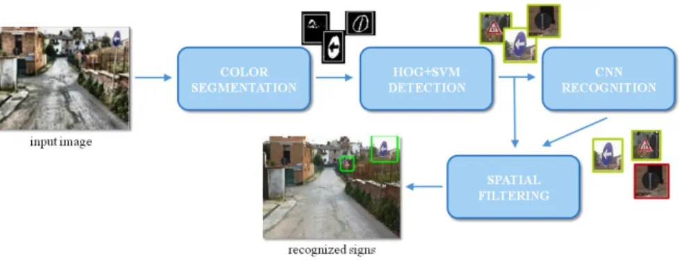
The functional architecture of the proposed approach is shown in Fig. 1. At the beginning, a color segmentation step is used for reducing the search space. The regions of the input image having color attributes similar to the road sign models are selected, creating an initial set of regions of interest (ROIs). Then, features
2
Fig. 1. The proposed pipeline for automatic traffic sign detection and recognition. Image best viewed in color.
are extracted from each ROI and represented as HOG descriptors. After that, a multi-scale detection process, based on a trained SVM model, takes place. Information about the position and the size of each possible sign are stored for being used later. At the same time, each detection is passed to the CNN based recognition module: If a sign is successfully assigned to a class, it is sent to the final stage of the procedure, otherwise it is processed by using a probabilistic spatial filtering, whose probabilities are computed among adjacent ROIs. The ROIs that passed all the processing phases are labeled as recognized signs. 3.1 Traffic Sign Detection
We use a combination of color and shape-based methods for detecting the signs. The shape-based method includes normalizing operations in addition to multi-scale image processing, in order to handle the challenges presented in a typical street scene. Since the pixels belonging to traffic signs usually represent a small percentage of all the pixels in input, it is desirable to reduce the initial search space. According to [6], we assume that traffic signs have bright and saturated colors, in contrast with the surrounding environment, to be recognized easily by drivers. This assumption helps in covering with the detection windows only a small subset of the patches extracted from the original image.
The extraction of the ROIs is carried out by utilizing the Improved Hue, Saturation, and Luminance (IHSL) color space [8], which is useful for taking into account lighting changes since the chromatic and achromatic components are independent in IHSL. The original image is transformed from RGB to IHSL by applying the following thresholding operation:
IHSL(x, y) = 0,if M ax(IR(x, y), IG(x, y), IB(x, y)) =IG(x, y) ∨ (|IR(x, y)−IG(x, y)|< ζ ∧ |IB(x, y)−IG(x, y)|< γ) Fihsl(IR(x, y), IG(x, y), IB(x, y)), otherwise (1)
where IHSL(x, y) is the IHSL color space value for the pixel in position (x, y), havingIR, IG, andIB RGB values. The function Fihsl(.) represents the
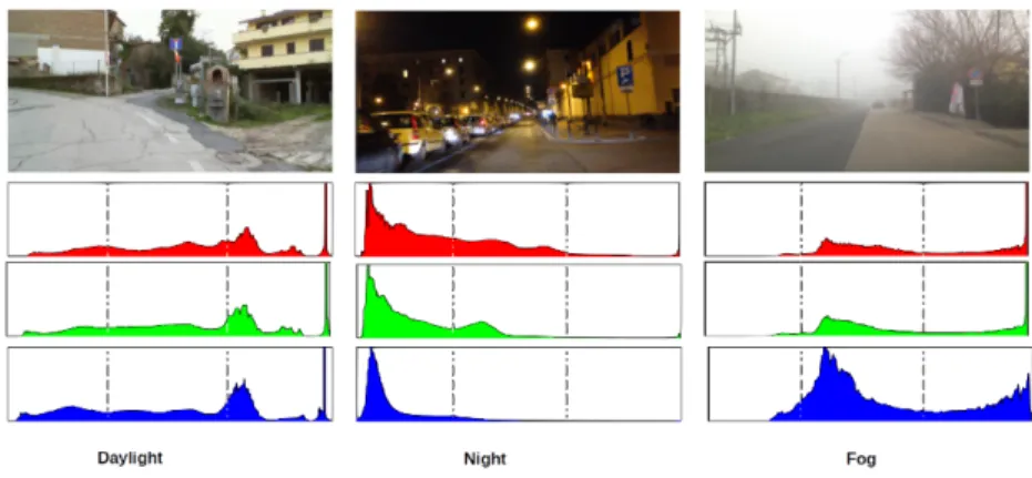
Fig. 2. The color histogram of the three types of scenes. The dashed lines represents the three different areas considered over each histogram. This image is best viewed in color.
usual conversionRGBcolorspace→IHSLcolorspaceas described in [7]. It is worth noting that RGB pixels with a considerable percentage of green (e.g., represent-ing vegetation) are discarded. Theζ and γ thresholds play a significant role in filtering out further pixels (e.g., belonging to road and sky), thus reducing the computational time for the IHSL conversion and the subsequent detection steps. The values forζandγ are set based on the lighting conditions in the scene: the color distribution represented by the RGB histogram is used to detect the illumination conditions (see Fig. 2). Each RGB histogram is divided into three equal areas. This division helps to determine where the color information is condensed and to locate the peak value in each histogram. In daylight conditions, the color information distribution is located in the right area of the histogram, with peak values at the most right side. Night-time scenes have a higher number of pixels located within the left area, while in foggy conditions the greater number of pixels is distributed over the middle and right areas. More formally, the color distribution over each histogram area is computed as:
n= P nH(i), if H(i)≥α P ∀nH(i) (2)
where n represents the distribution of each RGB color channel over one of the three areas (n ∈ {1,2,3}), H(i) is the number of pixels with color value
i ∈ [0,255], and α is set to 0.3∗max(H(i)),∀i. The maximum n is used to detect the lighting condition of the scene and to adapt the values of γ and ζ
according to it.
The final binary image is computed by applying the approach described in [18], where the Normalized Hue-Saturation (NHS) method and post-processing steps are used to find the potential pixels belonging to road signs. Erosion and dilation morphological operators are applied on the binary image for noise re-moval. The remaining pixels are grouped into contours, which in turns are filtered according to their size. The bounding box of each extracted contour is computed and clustered into spatial-classes according to the distances and the overlapping
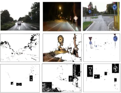
Fig. 3.Color segmentation and contour extraction. Original images are in the first row. The second row shows the results of the RGB thresholding, while the third row contains the contour extraction. In the first columnζ= 15 andγ= 25 are used, in the secondζ= 40 andγ= 25 and in the third
ζ= 15 andγ= 20.
of each bounding box. This procedure is useful for handling partially occluded, with multiple colors, or damaged road signs. Fig. 3 shows the color segmenta-tion along with the contour extracsegmenta-tion procedure that led to the extracsegmenta-tion of the patches (highlighted in the last row of the figure).
Visual descriptors are then computed over the extracted patches. For HOG, we use a 40×40 detection window with 10×10 block size and 2×2 striding. Three rounds of training are performed in total, adding hard negatives to the training images in every round. For the first round, we used GTSRB positives samples along with custom negatives: around 2000 samples were added. In the second round, the same procedure has been applied to DITS data. Positives samples from both GTSRB and DITS together with all the collected hard negatives from the previous steps are used for the last round of training. The color segmentation stage helps in decreasing the false positive detection and to accelerate the overall procedure.
3.2 Traffic Sign Recognition
Our recognition module is based on CNN and built over the Deep Learning framework TensorFlow. All images are down-sampled to 28×28. For both DITS and GTSRB, also jitter (augmented) samples are used. Images are randomly rotated, scaled and translated. Max values for the perturbations are [−15,15] for rotation, [−4,4] for translation and a factor [0.8,1.2] for scaling. The augmented data set is four times bigger than the original.
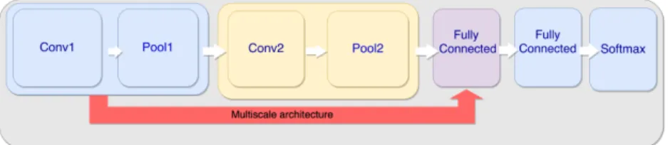
Fig. 4.Proposed architecture for CNN. In case of multiscale architecture, the output of the first convolutional layer feeds both the second convolutional layer and the first fully connected one.
The Deep Learning approach has two different architectures (see Fig. 4), a Single-Scale Convolutional Neural Network and a modified version of the Multi-Scale architecture proposed by Sermanet et al. for the GTSRB competition. The single-scale architecture presents two convolutional layers, each one followed by a pooling layer, and two sequential fully connected layer with rectification. The last layer is a softmax linear classifier. The multi-scale CNN is based on both the work by Sermanet and LeCun [13] and the single-scale architecture above described. The model presents two stages of convolutional layers, two local fully connected layer with rectified linear activation and a softmax classifier. As for the single-scale case, each convolutional layer presents a pooling layer. The output of the first convolutional stage has two ramifications, one feeds the next stage in a feed-forward fashion, while the other serves as part of the input for the first of the fully connected layer. The input of such layer is built from the output of the first stage and the output of the second stage.
3.3 Spatial Neighbourhood Filtering
The last module of our pipeline is in charge of fusing information from the detection module and the classification one. Algorithm 1 contains the details about this last step. A probability value is assigned to each one of the patches that are not recognized as a specific traffic sign, taking into consideration their position and their neighbour patches.
Algorithm 1: Spatial Neighbourhood Filtering Input :unrecognised detectionsα, recognized detectionsβ.
Output:Accepted detection
1 for∀d: d∈βdo
2 1: M←maximum rangeford;
3 2:for∀c: c∈α∧c in rangeM do 4 i:pd←compareSize (d,c); 5 ii:pd←compareDistance (d,c); 6 end 7 3:if pd> thresholdthen 8 accept d; 9 else 10 discard d; 11 end 12 end
A thresholding process is further applied over the final probabilities to filter out untrusted patches from the final list. It is worth noting that in real appli-cations, such as driver assistance systems, the driver should not be warned due to false detections. Indeed, although the proposed solution helps to increase the accuracy by 1-2% depending on the data set, it strongly relies on the recognition sub-systems, adding a small probability to discard correct detections.
The output of the classification module is divided intoclassified detections (i.e., the detections successfully assigned to a class by the CNN) andnot-classified ones. For every element in the not-classified detection set, we define a search range around it and compute, for every sample in the classified set that lies within the range, the following two metrics: (i) the similarity between the size of the not-classified and the classified element and (ii) the distance between the center of the two elements. If the sum of the two above listed comparison metrics is below a given threshold, then the not-classified detection is definitively discarded, otherwise it is accepted.
4
THE DATA SET OF ITALIAN TRAFFIC SIGNS
Since the release of the German Traffic Sign Data set (GTSRB) in 2011, no other challenging data sets have been released. According to Mathias et al. [10], the GTSRB have been saturated and there is the need of novel public and more complex data sets. Here, we present the Data set of Italian Traffic Signs (DITS), which is a novel data set, generated in part from HD videos (1280×720 frame size recorded at 10 fps) taken from a commercial web-cam and different smart phones. DITS data can be downloaded at: http://www.dis.uniroma1. it/~bloisi/ds/dits.html
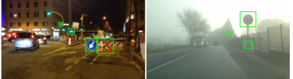
The aim of DITS is to provide more challenging images than its predecessors. First, not all the used sensors are intended for outdoor shooting and the quality of the images is lower if compared with the one in GTSRB. As suggested in [10], we have increased the difficulty by adding images captured at night time and in presence of fog (see Fig. 5). A big part of the samples contains complex urban environments that can increase the presence of false positives. Finally, DITS presents a new challenging class of traffic signs, named Indication, which
Fig. 5.Two annotated images from the DITS data set captured at night time (left) and with fog conditions (right). Annotations are shown in green.
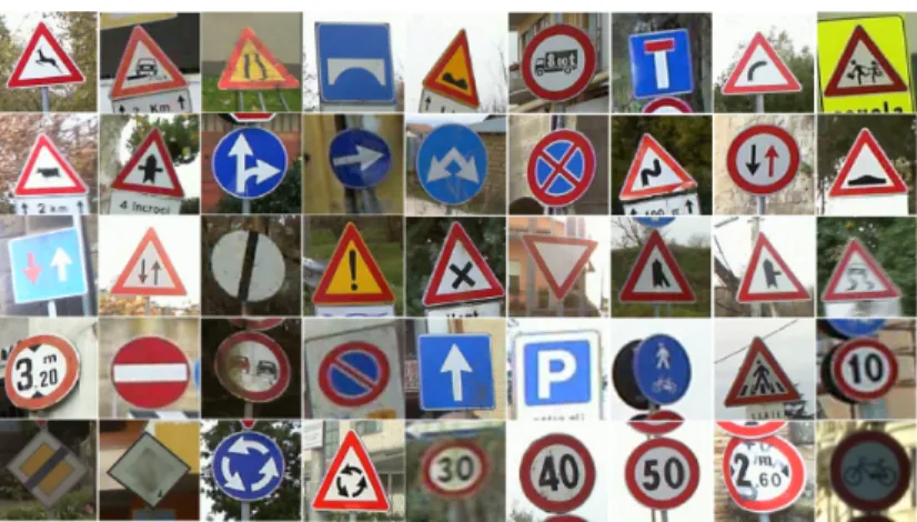
Fig. 6. Images from the classification sub set of the DITS data set. DITS contains 58 different classes.
includes square-like traffic signs. Both detection and classification training and test sets are present. The detection subset offers 1,416 images for training and 471 for testing, while the classification subset contains 8,048 samples for training and 1,206 for testing. Currently, DITS is at an early stage and our plan is to improve it in the next few months.
DITS has been originally generated from 43,289 images extracted from more than 14 hours of videos recorded in different places around Italy. Images are then down-sampled to fullfill the following requirements. All the images in the data set are enclosed in classes. In particular, training images for both detection and classification are organized in folders, where each folder represents a single superclass or sub-class. Annotated images are available for testing and text files with more accurate information and annotations are provided.
About the detection subset, we decided to define three shape-based super-classes, namely circle, square, and triangle, obtaining the Prohibitive, Indication, and Warning classes. The bottom threshold for the width and the height of the samples present is set to 40 pixels for both; images are not necessarily squared. The classification data set presents 58 classes of signs: each class presents a vari-able number of tracks where the concept of track collide with the one previously used in GTSRB [14]. The difference with the GTSRB is on the number of images present in each track (15) and mainly dictated by the lower frame rate offered by the sensor used. Tracks presenting a higher number of images are downsized by equidistant samples; tracks with less than 15 samples are discarded. Images in the track have different size and, as for the detection subset, they may vary in aspect ratio. Fig. 6 shows some samples coming from the classification test set.
5
EXPERIMENTAL RESULTS
The approach proposed in this paper has been tested on two different publicly available data sets, the German Traffic Sign Data set (GTSRB) and the Data
Table 1.Comparison results on the GTSRB data set of our approach with and without activating the color segmentation (ColSeg).
Method Prohibitive Danger Mandatory AUC ∼Time(ms) AUC ∼Time(ms) AUC ∼Time(ms) HOG 96.33% 693 96.12% 693 89.18% 693 ColSeg+HOG98.67% 231 96.01% 234 90.43% 243
Table 2.Results on the DITS data set with and without color segmentation (ColSeg).
Method Prohibitive Danger Indication AUC ∼Time(ms) AUC ∼Time(ms) AUC ∼Time(ms) HOG 96.63% 615 98.00% 615 81.06% 615 ColSeg+HOG97.87% 198 98.12% 197 89.71% 200
set of Italian Traffic Signs (DITS). We have evaluated the proposed approach for detection on 300 images coming from GTSRB and 471 from DITS. The two data sets present some differences: (i) only the Danger superclass has a direct correspondence;(ii) the Mandatory and Prohibitive superclasses of GTSRB are merged into the Prohibitive superclass for DITS;(iii)DITS has a new Indication superclass (i.e., square signs).
For both the German and the Italian data sets, we have tuned the param-eters according to the different settings of the sensors. Most of the images in GTSRB present a saturated blue sky and low saturation on the red, translat-ing into a slightly higher value onγ, while DITS data present a less saturated sky in daylight conditions, while night time images present alterations over the red and blue channels. Night time images present also a lower accuracy of the color segmentation process, thus lowering the performance in subsequent phases. Common street lamps have a color temperature that ranges between 2000 and 3000 Kelvin and this reduces the area discarded by the red-based threshold. Moreover, car headlights cause a sudden change in brightness that blur the im-age. In this case, we setζ= 40 andγ= 25. Fog affects the segmentation process, slightly increasing the false negative rate. For fog images, we have used ζ = 5 andγ= 5.
After the tuning, results show that we are able to discard, on average, 82% of the pixels for the images in DITS and 69% for GTSRB data. This strong reduction allows the next stage of the detection sub-system to process a smaller portion of the original image, speeding up the analysis up to 5 times. Table 1 and Table 2 show the improvements in accuracy and computational time that can be obtained by using a pre-classification step based on color segmentation. Our method obtains comparable results with others existing methods (see [19] for results obtained by other approaches on GTSDB). Experimental results on DITS show even higher speed than those obtained on GTSRB. The lower accuracy
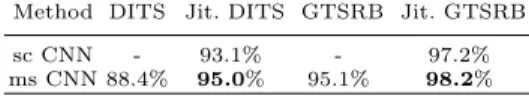
Table 3.Recognition results with single scale (sc) and multi scale (ms) CNN.
Method DITS Jit. DITS GTSRB Jit. GTSRB sc CNN - 93.1% - 97.2% ms CNN 88.4% 95.0% 95.1% 98.2%
when dealing with the new Indication superclass is due to the high presence of false positive in urban environment (e.g., square-like object as windows).
Classification results are shown in Table 3. Results for DITS data are com-pletely new and not comparable. On the GTSRB we reached good results if compared with those previously published on the German Traffic Sign Recogni-tion Benchmark page (http://benchmark.ini.rub.de).
The accuracy of the proposed pipeline (detection+classification+spatial fil-tering) has been evaluated on DITS data. For the detection process, we started from an overall accuracy of 95.23%, while the recognition subsystem consists in the single-scale Convolutional Neural Network trained on the jittered data set. From 347 outputs from the detection, 93% samples have been successfully assigned to a class. The remaining 7% is processed by our Spatial Neighborhood Filter to mitigate the error of the classifier. Results show that 1.2% samples are confirmed, while the other are discarded as false positives. Among the confirmed samples, only the 0.2% resulted in false positives.
6
CONCLUSIONS
In this paper, we have described a fast and accurate pipeline for road sign recog-nition. The proposed approach combines different state-of-the-art methods ob-taining competitive results on both detection and classification of traffic signs. Particular attention has been given to the detection phase, where color segmen-tation is used to reduce the portion of the image to process, thus reducing the computational time.
Quantitative experimental results show an 82% average reduction of the search space, which speed up the process without affecting the detection accu-racy. The CNN architecture allows to further discard false positives by combining the outputs from the detection and the recognition modules.
Moreover, we have presented a novel data set, called the Data set of Italian Traffic Signs (DITS), which presents some innovations over existing data sets, such as night-time and complex urban scenes. Since available data sets already reached saturation (over 99% accuracy), we believe that the development of a novel data set with more challenging data is an important contribution of this work. As future directions, we intend to extend DITS with additional images, captured under adverse weather conditions (e.g., rain and snow).
References
1. N. Barnes and A. Zelinsky. Real-time radial symmetry for speed sign detection. InIntelligent Vehicles Symposium, pages 566–571, 2004.
2. R. Benenson, M. Mathias, R. Timofte, and L. Van Gool. Pedestrian detection at 100 frames per second. InCVPR, pages 2903–2910, 2012.
3. D.C. Ciresan, U. Meier, J. Masci, and J. Schmidhuber. Multi-column deep neural network for traffic sign classification. Neural Networks, pages 333–338, 2012. 4. P. Doll´ar, Z. Tu, P. Perona, and S. Belongie. Integral channel features. InBMVC,
2009.
5. P. Dollr, R. Appel, and W. Kienzle. Crosstalk cascades for frame-rate pedestrian detection. InECCV, pages 645–659, 2012.
6. K. Doman, D. Deguchi, T. Takahashi, Y. Mekada, I. Ide, H. Murase, and U. Sakai. Estimation of traffic sign visibility considering local and global features in a driving environment. InIntelligent Vehicles Symposium, pages 202–207, 2014.
7. H. Fleyeh. Color detection and segmentation for road and traffic signs. In Cyber-netics and Intelligent Systems, 2004 IEEE Conference on, pages 809–814, 2004. 8. A. Hanbury. A 3d-polar coordinate colour representation well adapted to image
analysis. InImage Analysis, pages 804–811, 2003.
9. A. Krizhevsky, I. Sutskever, and G.E. Hinton. Imagenet classification with deep convolutional neural networks. InAdvances in neural information processing sys-tems, pages 1097–1105, 2012.
10. M. Mathias, R. Timofte, R. Benenson, and L. Van Gool. Traffic sign recognitionhow far are we from the solution? InIJCNN, pages 1–8, 2013.
11. G. Overett, L. Tychsen-Smith, L. Petersson, N. Pettersson, and L. Andersson. Creating robust high-throughput traffic sign detectors using centre-surround hog statistics. Machine vision and applications, pages 713–726, 2014.
12. P. Perona. Visual Recognition, Circa 2007. In Object Categorization Computer and Human Vision Perspectives, pages 55–68. Cambridge University Press, 2009. 13. P. Sermanet and Y. LeCun. Traffic sign recognition with multi-scale convolutional
networks. InIJCNN, pages 2809–2813, 2011.
14. J. Stallkamp, M. Schlipsing, J. Salmen, and C. Igel. Man vs. computer: Bench-marking machine learning algorithms for traffic sign recognition. Neural Networks, pages 323 – 332, 2012.
15. M. Tan, B. Wang, Z. Wu, J. Wang, and G. Pan. Weakly supervised metric learning for traffic sign recognition in a LIDAR-equipped vehicle. IEEE Transactions on Intelligent Transportation Systems, 17(5):1415–1427, 2016.
16. R. Timofte and L. van Gool. Sparse representation based projections. InBMVC, pages 61.1–61.12, 2011.
17. R. Timofte and L. van Gool. Iterative nearest neighbors for classification and dimensionality reduction. InCVPR, pages 2456–2463, 2012.
18. Valentine Vega, D´esir´e Sidib´e, and Yohan Fougerolle. Road signs detection and reconstruction using gielis curves. InInternational Conference on Computer Vision Theory and Applications, pages 393–396, 2012.
19. D. Wang, S. Yue, J. Xu, X. Hou, and C.-L. Liu. A saliency-based cascade method for fast traffic sign detection. In Intelligent Vehicles Symposium, pages 180–185, 2015.
20. Y. Zeng, X. Xu, Y. Fang, and K. Zhao. Traffic sign recognition using deep con-volutional networks and extreme learning machine. In IScIDE, pages 272–280, 2015.