Context-specific subcellular localization prediction: Leveraging protein interaction networks and scientific texts

(1)

Context-specific subcellular localization

prediction: Leveraging protein

interaction networks and scientific texts

Lu Zhu

Bielefeld University

This dissertation is submitted for the degree of

Doctor rerum naturalium

(2)

Lu Zhu

Context-specific subcellular localization prediction: Leveraging protein interaction networks and scientific texts

Bioinformatics & Medical Informatics Department

German-Canadian DFG International Research Training Group (1906/1) Faculty of Technology, Bielefeld University

Referees:

Prof. Dr. Ralf Hofestädt

Bioinformatics & Medical Informatics Department Bielefeld University, Germany

Prof. Dr. Martin Ester

School of Computing Science Simon Fraser University, Canada

Dr. William J Duddy

Northern Ireland Center for Stratified Medicine Ulster University, Northern Ireland

(3)

Acknowledgements

I express my deep sense of gratitude and appreciation to my advisors Prof. Dr. Ralf Hofestädt and Prof. Dr. Martin Ester for all of their support of my doctoral study and related research, for their patience, constant encouragement, and expert guidance.

Besides my advisor, I would like to thank the rest of my thesis committee for their insightful comments and encouragement, but also for the inspiring questions which incented me to widen my research from various perspectives.

My sincere thanks also go to Frank Grimm and Tobias Tekath for the stimulating dis-cussions and the contribution to the text mining project in this dissertation. Without their precious support, it would not be possible to conduct this research task.

I would like to acknowledge funding from the international research training group GRK/1906 “Computational Methods for the Analysis of the Diversity and Dynamics of Genomes” (DiDy) for three years, and scholarship from the bioinformatics and medical informatics research group for the past months.

I am also grateful to my colleagues and friends who have supported and encouraged me along the way.

Last but not the least, I would like to thank my family: my parents and my sister for supporting me spiritually throughout writing this thesis and my life.

(4)

(5)

Abstract

One essential task in proteomics analysis is to explore the functions of proteins in conducting and regulating the activities at the subcellular level. Compartmentalization of cells allows proteins to perform their activities efficiently. A protein functions correctly only if it occurs at the right place, at the right time, and interacts with the right molecules. Therefore, the knowledge of protein subcellular localization (SCL) can provide valuable insights for understanding protein functions and related cellular mechanisms. Thus, the systematic study of the subcellular distribution of human proteins is an essential task for fully characterizing the human proteome.

The context-specific analysis is an important and challenging task in systems biology research. Proteins may perform different functions at different subcellular compartments (SCCs). Hence, the dynamic and context-specific alterations of the subcellular spatial distribution of proteins are essential in identifying cellular function. While this important feature is well-known in molecular and cell biology, most large-scale protein annotation studies to-date have ignored it.

Tissue is one particularly crucial biological context for human biology. Proteins show their tissue specificity at the subcellular level by localizing to different SCCs in different tissues. For example, glutamine synthetase localizes in mitochondria in liver cells while in the cytoplasm in brain cells. The knowledge of the tissue-specific SCLs can enrich the human protein annotation, and thus will increase our understanding of human biology.

Conventional wet-lab experiments are used to determine the SCL of proteins. Due to the expense and low-throughput of wet-lab experimental approaches, various algorithms and tools have been developed for predicting protein SCLs by integrating biological background knowledge into machine learning methods. Most of the existing approaches are designed for handling general genome-wide large-scale analysis. Thus, they cannot be used for context-specific analysis of protein SCL.

The focus of this work is to develop new methods to perform tissue-specific SCL pre-diction. (1) First, we developed Bayesian collective Markov Random Fields (BCMRFs) to address the general multi-SCL problem. BCMRFs integrate both protein-protein interaction network (PPIN) features and the protein sequence features, consider the spatial adjacency of

(6)

SCCs, and employ transductive learning on imbalanced SCL data sets. Our experimental results show that BCMRFs achieve higher performance in comparison with the state-of-art protein-protein interaction (PPI)-based method in SCL prediction. (2) We then integrated BCMRFs into a novel end-to-end computational approach to perform tissue-specific SCL pre-diction on tissue-specific PPINs. In total, 1314 proteins which SCLs were previously proven cell lines dependent were successfully localized based on nine tissue-specific PPINs. Fur-thermore, 549 new tissue-specific localized candidate proteins were predicted and confirmed by scientific literature. Due to the high performance of BCMRFs on known tissue-specific proteins, these are excellent candidates for further wet-lab experimental validation. (3) In addition to the proteomics data, the existing scientific literature contains an abundance of tissue-specific SCL data. To collect these data, we developed a scoring-based text mining system and extracted tissue-specific SCL associations from the abstracts of a large number of biomedical papers. The obtained data are accessible from the web based database TS-SCL DB. (4) We concluded the study with an application case study of the tissue-specific subcel-lular distribution of human argonaute-2 (AGO2) protein. We demonstrated how to perform tissue-specific SCL prediction on AGO2-related PPINs. Most of the resulting tissue-specific SCLs are confirmed by literature results available in TS-SCL DB.

(7)

List of figures

2.1 Schematic overview of the animal cell. . . 9

2.2 Schematic overview of intracellular protein trafficking. . . 11

2.3 Physical contact between two proteins. . . 13

2.4 Relation of types based on affinity and stability. . . 14

2.5 Example of simple graphs. . . 15

2.6 Co-expression network inference pipeline. . . 22

2.7 Pipeline of text mining solution. . . 23

3.1 Protein-protein interaction network as an undirected graph. . . 30

3.2 Indirect neighbors in protein-protein interaction network. . . 33

4.1 Binarization of multi-label MRFs. . . 43

4.2 Overview of the collective MRFs. . . 50

4.3 The overview of implementation of BCMRFs method. . . 57

4.4 Summarization of descriptive data from the human protein dataset. . . 58

4.5 Characters of PPIN dataset. . . 58

4.6 Relationship between the likelihood and prediction performance. . . 59

4.7 Performances of BCMRFs during iterations. . . 59

4.8 Imbalance level of each SCL class. . . 60

4.9 Prediction performances of four models. . . 61

5.1 The workflow of the tissue-specific SCL prediction based on PPINs. . . 65

5.2 The overview of implementation of tissue-specific BCMRFs method. . . 68

5.3 The property of the tissue-specific physical PPINs. . . 80

5.4 Comparison of protein SCLs across tissues. . . 81

5.5 Impact of tissue-specific functional association on performance. . . 82

6.1 Schematic diagram of the text mining system . . . 86

(12)

6.3 SCL mapping along the GO tree. . . 94

6.4 Benchmark of tissue-protein-SCL association obtained through text mining. 97 6.5 Histogram bar chart of scored true positive triplets and negative positives. . 97

6.6 Tuning the scoring parameters. . . 98

6.7 Comparison of the text-mined results with HPA experimentally validated cell line data. . . 100

6.8 Distribution of the scored triple association. . . 100

6.9 Illustration of web interface. . . 106

7.1 Best connected tissue-specific PPINs of human AGO2 protein. . . 118

7.2 The subcellular distribution of the interacting proteins of AGO2 across tissues.119 7.3 The predicting subcellular distribution of human AGO2 across tissues. . . . 121

(13)

List of tables

4.1 F1 scores with/without imbalance correction. . . 55

4.2 F1 scores for transductive VS conventional. . . 55

4.3 Comparison with the method of DC-kNN - Multi-SCL prediction. . . 56

4.4 Comparison with the method of Hum-mPLoc 3.0 - Multi-SCL prediction. . 56

5.1 Mapping table from cell lines to tissues. . . 69

5.2 The imbalance level of SCL dataset across tissues. . . 72

5.3 The distribution of protein SCL across tissues. . . 72

5.4 tissue-specific multi-SCL prediction performance. . . 77

6.1 Performance of text mining system for triplet prediction . . . 96

6.2 Accuracy of overlapped triplets. . . 101

6.3 Overview of TS-SCL database. . . 102

7.1 Interacting partners of AGO2 . . . 111

(14)

(15)

Chapter 1 Introduction

1.1 Understanding protein subcellular localizations

One essential task in proteomics analysis is to explore the functions of protein in conducting and regulating the activities at the subcellular level [1]. As the eukaryotic cells and particularly the mammalian cells are highly compartmentalized, most protein activities can be assigned to particular cellular compartments. It is well known that protein functional activities highly correspond with their subcellular distribution and molecular complexing interactions [2]. A protein functions correctly only if it occurs at the right place, at the right time, and interacts with the right molecules. In other words, the functions of protein and protein interactions rely greatly on the proper localization of each protein component [3, 4]. On the other hand, the aberrant translocalization of proteins often correlates with pathological changes in cell physiology and accounts for a variety of human diseases such as Alzheimer’s disease, Swyer syndrome, and various type of cancer. Hence, the mislocalization of protein makes protein translocalization a promising target for the development of therapeutic agents [5]. Therefore, the knowledge of protein SCL can provide valuable insights for understanding protein functions and related cellular mechanisms. Hence, the systematic study of protein SCLs is essential for fully characterizing the human proteome, and a major research topic in biology.

After synthesis of protein, protein can be transported into different subcellular com-partments (SCCs) depending on the roles within the cell. Such translocalization of protein accomplishes the transport of material and information within and between cells. Thus, it is essential for the normal functioning of the cell. Some proteins are even transported to multiple sites simultaneously or once at the time when the protein is needed, e.g. moon-lighting proteins [6] and circadian clock proteins [7]. Some of the multi-localizing proteins (MLPs) are also multi-functional proteins (MFPs), e.g. Enolase 1 fulfills different functions

(16)

in the cytosol and plasma membrane. The existence of MFPs and MLPs increases the cellular complexity because they can participate in multiple pathways or serve as regulators of transcription.

1.2 The importance of the context-specific subcellular

dis-tribution of proteins

The context-specific analysis is an important and challenging task in systems biology research, such as study on tissue-specific expression of protein of human body [8], identification of disease-specific protein-protein interaction (PPI) [9, 10], prediction of the temporal organization of cellular functions using the dynamic circadian protein-protein interaction networks (PPINs) [11], the analysis the SCL of protein under stress condition [12].

The protein function is highly dependent on the spatial distribution of many cellular com-ponents under various types of biological event, e.g. tumorigenesis [13], cellular apoptotic activity [14], and environments, e.g. stress [12], different tissues [15–17]. An example of crucial subcellular distribution is breast cancer type 1 susceptibility protein (BRCA1), well known for its nuclear, cytoplasmic trafficking in breast cancer [18]; recently, its redistribu-tion to the cytoplasm in malignant breast cancer tissues has been supposed to be a defense mechanism of the cell probably associated with a more intense cellular apoptotic activity [19]. Moreover, glutamine synthetase (GS) is mitochondrial in liver cells and cytoplasmic in brain cells [15]. In the human tissue adrenal gland, pituitary gland and pancreas, the absence of adracalin (ALADIN) in nuclear membrane causes human triple A syndrome [16]. The dynamic alterations of subcellular spatial distribution of proteins are at least equally important to changes in total protein abundance in cellular function. However, this essential feature is long known from molecular and cell biology, but so far is often ignored in many large-scale studies. The emerging theme, which is the focus of this work, is to understand the dynamic and context specific subcellular distribution of protein.

1.3 Computational prediction of protein subcellular

local-ization

Conventional wet-lab experiments are used to determine the SCLs of protein. The most popular wet-lab approaches such as electron microscopy, quantitative mass-spectrometric, and immunofluorescence (IF) combined with confocal microscopy are expensive and time-consuming. Unfortunately, the SCLs of a majority of proteome still remains unknown.

(17)

1.3 Computational prediction of protein subcellular localization 3

Owing to the automated and high-throughput nature, computational methods are appeal-ing for the large-scale assignment of protein SCLs. Scientists have made extensive efforts to develop efficient approaches for analyzing the SCL of protein. Various algorithms and tools have been developed for predicting protein SCLs by integrating biological background knowledge into machine learning methods. Those predictions are made from the information such as protein amino acid sequence, functional domains, and motifs, protein-protein interac-tion (PPI), Gene Ontology (GO) annotainterac-tions of protein, protein homology, key informainterac-tion in scientific texts, either unitarily or combined.

The existing methods have their unique strengths and disadvantages. The common limitation is that they mainly focus on the static studies of the tissue-generic subcellular distribution of the protein. Sequence-based prediction methods have been successfully used in genome-wide large-scale protein SCL annotation. However, the primary sequence of protein always reminds the same, even though the protein could have been translocated by binding to other molecules. Thus, those methods can not be applied to determine the translocalization of protein. It was shown that using the protein annotation information and protein interactions can increase the accuracy of protein SCL prediction [20, 21]. However, the existing approaches are lack of context specificity. For instance, the PPI which occurs only in brain tissue should not be used for predicting the SCL in the other tissue. The SCLs which were determined in a healthy sample might be not applicable to a study in cancer context. Using unspecified data in a context-specific study can produce unreliable results in SCL prediction. Hence, there is still room to improve in protein SCL prediction. Furthermore, the blankness of the computational approach for the systematic analysis of the protein context-specific SCL is required to be filled.

Argonaute-2 (AGO2) protein is a key player in gene-silencing pathways. It has been mostly known as a cytoplasmic protein [22]. However, more recent studies and data sug-gested that AGO2 is a MLP [23–26]. AGO2 is also a MFP which is involved in different biological events such as mRNAs degradation, mRNA splicing event, translation repression. Furthermore, Sharma et al. [17] demonstrated that the nuclear distribution of AGO2 occurs in a cell type- and tissue context-dependent manner. Hence, we believe that the various func-tions of AGO2 may correlate to its SCLs and the tissue where it expresses. A tissue-specific analysis of the subcellular distribution of AGO2 protein helps to understand its functions better.

(18)

1.4 The aim of this work

This work aims to develop efficient methods for protein tissue-specific SCLs analysis. The major components of this research are summarized in below.

• First, we developed BCMRFs to address the general multi-SCL problem. BCMRFs integrate both PPIN features and the protein features, consider the spatial adjacency of SCCs, and employ transductive learning on imbalanced SCL data sets. Our experi-mental results show that BCMRFs achieve higher performance in comparison with the state-of-art PPI-based method in SCL prediction.

• We then integrated BCMRFs into a novel end-to-end computational approach to per-form tissue-specific SCL prediction on tissue-specific PPINs. In total, 1314 proteins which were known to localize to different SCCs in different tissues and cell lines were successfully localized. Furthermore, 549 new tissue-specific localized candi-date proteins were predicted. Due to the high performance of BCMRFs on known tissue-specific proteins, these are excellent candidates for further wet-lab experimental validation.

• In addition to the proteomics data, the existing scientific literature contains an abun-dance of tissue-specific SCL data. To collect these data, we developed a scoring model based text mining system and extracted tissue-specific SCL associations from the abstracts of a large number of biomedical papers. The obtained data are accessible from our web-based TS-SCL database.

• We concluded the study with an application case study of the tissue-specific subcellular distribution of human AGO2 protein. We demonstrated how to perform tissue-specific SCL prediction on AGO2-related PPINs. Most of the resulting tissue-specific SCLs are confirmed by literature results available in our TS-SCL database.

1.5 Structure of this work

The dissertation is organized as follows. In Chapter 2, we begin with the fundamental knowledge which is necessary to understand this thesis. The first section introduces the cellular compartmentalization, the significance of proteins SCLs, protein translocalization event for the understanding of cellular mechanisms. One of the important tasks of this work is the prediction of protein SCLs by leveraging the PPI data using probabilistic graphical model. Thus, we explained the definition of PPI, PPIN, and major data resource and the data

(19)

1.5 Structure of this work 5

reliability. Furthermore, to better understand our approaches, we recalled the basic concept of graph theory including Markov random field (MRF), Bayesian inference, Gibbs sampler, and the multi-label classification problem. In the last part of this chapter, we elucidated the data curation process using text mining technology in a nutshell.

Chapter 3 reviews the existing popular methods for experimentally detecting and compu-tationally predicting protein SCLs. These approaches were compared from the perspectives of biological concepts, machine learning method. The limitations were also discussed includ-ing the issue of multi-label classification and the challenge of performinclud-ing context-specific prediction. We described the rationale of using MRF on PPINs for protein SCL prediction. Finally, we brought out the importance of understanding the tissue-specific SCL of human proteins, and the current absence of a computational solution.

The next chapter, Chapter 4, illustrates how to improve the prediction performance of predicting multi-SCL of human MLPs in general. At first, we explained the motivation and the general idea of the approach using multi-label MRF. Next, we introduced our BCMRFs algorithm and the corresponding learning procedure. Section 4.2 details the experimental design and Section 4.3 shows the experimental results. At last, we summarized this task along with the discussion and limitations.

Chapter 5 demonstrates how to apply BCMRFs to specific PPINs for tissue-specific SCL prediction. We discussed the rationale of using tissue-tissue-specific PPINs for predicting protein tissue-specificSCL. This chapter also points out the challenge of lacking tissue-specific SCL original (’ground truth’) dataset for evaluation, and provide the detailed solution. After the evaluation of the method, a large-scale analysis of tissue-specific SCL prediction for human proteome was performed.

Next, Chapter 6 presents the text mining system which is able to extract the tissue-specific SCL from scientific literature. It demonstrates a method which uses a dictionary-based approach to extract and score the triple association of tissue, protein, and SCL. The method was validated with the manually curated gold standard corpus. Thereafter, we performed a large-scale extraction against PubMed abstracts. The resulting protein tissue-specific SCL data were stored in the web-based database, TS-SCL DB, together with the experimental, knowledge-based and predicted tissue-specific SCL data.

Additionally, as important as large-scale analysis, Chapter 7 illustrates how to perform tissue-specific analysis focusing on a protein of interest. In Chapter 7, we profoundly analyzed the subcellular distribution of human AGO2 based on tissue-specific PPIs and scientific literature . The resulting tissue-specific SCLs help us to understand the specific function of AGO2 across tissues and cell types.

(20)

In the end, all the achievements and the limitations were concluded in Chapter 8. The final chapters ends by addressing further directions for the work.

(21)

Chapter 2 Background

2.1 Subcellular localization

2.1.1 Cell and cellular compartmentalization

Cells are the basic units of life that facilitate and sustain every single process within a living organism. Cells are not an unstructured mixture of proteins, lipids, ions and other molecules. Instead, the cell creates subregions, each of which allows certain cell functions to operate more effectively. As such, the subdivision of cells into discrete subcellular compartments (SCCs) enables the cell to create specialized environments for specific functions.

Despite the morphological and functional variety of cells from different tissue types, all cells share essential similarities in their compartmental organization, such as the common SCCs plasma membrane, cytoplasm, and ribosomes. The plasma membrane is a phospholipid bilayer with proteins that separates the cell from the surrounding environment and functions as a selective barrier for the import and export of materials. The plasma membrane also helps contain the cytoplasm of the cell, which provides a gel-like environment for the cell’s organelles. The cytoplasm is the location for most cellular processes, including metabolism, protein folding, and internal transportation.

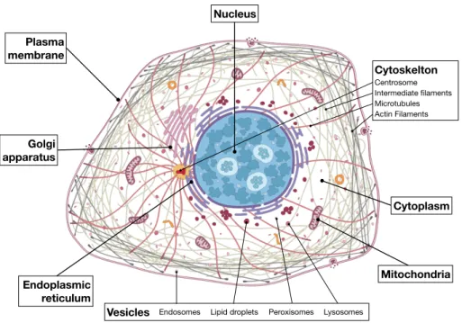
Unlike prokaryotic cells, eukaryotic cells (see Figure 2.1) have a nucleus enclosed within membranes. The nucleus houses the cell’s genetic material DNA that determines the entire structure and function of that cell. Ribosomes are responsible for protein synthesis. Often the distinction of SCCs is made between membrane-bound and non-membrane bound organelles. The membrane-bound organelles create a physical boundary thus separating the intra-and extra-organelle space.

• Mitochondria are oval-shaped, double membrane organelles that have their own ri-bosomes and DNA. These organelles are often called the “energy factories” of a cell

(22)

because they are responsible for making adenosine triphosphate (ATP), the cell’s primary energy-carrying molecule, by conducting cellular respiration.

• endoplasmic reticulum (ER) modifies proteins and synthesizes lipids, while the Golgi apparatus is where the sorting, tagging, packaging, and distribution of lipids and proteins takes place.

• Golgi apparatus is where the sorting, tagging, packaging, and distribution of lipids and proteins takes place. Golgi apparatus receives the entire output of de novo synthesized polypeptides from the ER and functions to posttranslationally process and sort them within vesicles destined to their proper final destination (e.g. plasma membrane, endosomes, lysosomes).

• Vesicles and vacuoles are membrane-bound organelles that function in storage and transport. Vacuoles are somewhat larger than vesicles, while the membranes of vesicles can fuse with either the plasma membrane or other membrane systems within the cell. • Lysosomes which contains a large number of hydrolytic enzymes that are used for

degrading almost any kind of cellular constituent, including entire organelles.

• Endosomes are involved in transport within the cell. They receive endocytosed cell membrane molecules and sort them for either degradation or recycling back to the cell surface. They also receive newly synthesized proteins destined for vacuolar/lysosomal. • Peroxisomes are small, round organelles enclosed by single membranes which carry

out oxidation reactions that break down fatty acids and amino acids.

In contrast, there are also non-membrane bound organelles such as the cytoskeleton and nucleoli.

• Cytoskeleton, including intermediate filaments, microfilaments, microtubules, the mi-crotrabecular lattice, and other structures not only serve in the maintenance of cellular shape but also have roles in other cellular functions, including cellular movement, cell division, endocytosis, and movement of organelles [27].

• The most prominent substructure within the nucleus is the nucleolus which is the site of ribosomal ribonucleic acid (rRNA) transcription and processing, and of ribosome assembly.

(23)

2.1 Subcellular localization 9 Golgi apparatus Nucleus Mitochondria Endoplasmic reticulum Cytoplasm Plasma membrane

Vesicles Endosomes Lipid droplets Peroxisomes Lysosomes

Cytoskelton

Centrosome

Intermediate filaments

Microtubules

Actin Filaments

Fig. 2.1Schematic overview of the animal cell. Eight primary SCCs, including Plasma membrane, Nucleus, Cytoplasm, Versicles, Mitochondria, Cytoskeleton, Endoplasmic reticulum, Golgi apparatus, and their substructures. Figure is adapted from Thul et al. [28].

2.1.2 Protein subcellular localization

For subcellular processes to be carried out within defined SCCs, mechanisms must exist to ensure the required protein components are present at the sites, at an adequate concentration and the correct timing. The accumulation of a protein at a given site is known as protein SCL.

One challenge in cell biology is how does the cell get materials (such as proteins, messenger ribonucleic acid (mRNA), ion) in and out across the membranes, and each compartment has its solution. The study of SCL and the transportation of the materials implicates many questions, such as: What controls the movement of a protein from one region to another? What does the protein-import material consist of? Which proteins are involved in mitochondria for instance (organelle proteome)?

The spatial partitioning of biological processes is a phenomenon fundamental to life that enables multiple processes to occur in parallel. SCLs direct the access of proteins to its interacting partners, such as other molecules and the post-translational modification machinery. Moreover, SCL is essential to protein function and its functional diversity [5].

(24)

Hence, resolving protein SCL, and the spatial distribution of the human proteome at a subcellular level can significantly increase our understanding of human biology.

2.1.3 Protein translocation

Protein translocation is a process by which proteins move between SCCs. It is a fundamental requirement for proteins to be able to exert their functions in different organelles. Short amino-acid sequences within a protein, known as signal peptides or signal sequences, can direct its localization, although translocation also occurs in the absence of these signal sequences. Protein translocation can occur co-translationally or post-translationally. Approximately half of the proteins generated by a cell have to be transported into or across at least one cellular membrane to reach their functional destination [29]. As a post-transcriptional process, some proteins translocate to the mitochondria, peroxisomes or the nucleus [30]. Whereas many proteins, including those destined for the secretory pathway and integral membrane proteins, are transported into the ER during synthesis, as the co-translational translocation [31].

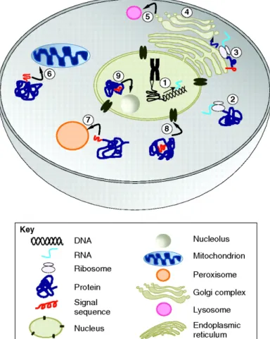
Protein translocation accomplishes the movement of material and information within the eukaryotic cell and is essential for the normal activity of the cell. The protein transport machinery of cells ensures that the right amount of protein is present at the right time and place. Hung and Link [5] summarized an overview of intracellular protein trafficking and an example of protein translocation induced by peptide signal, see Figure 2.2.

2.1.4 Multi-localizing protein

Owing to the translocation, proteins which are often localized to more than one organelle, which are called multi-localizing proteins (MLPs). MLPs present several advantages for the cell, some which are crucial for cellular survival.

The multilocation of protein often happens in the following translocation scenarios. Shuttle proteins continuously switch their SCL to transport other proteins between SCCs. For instance, importin α transports protein from the cytosol to the nucleus and thus is

found in both SCCs [32]. The proteins are involved in the reactions which take place in more than a single SCC, e.g. mitochondria and peroxisomes share some enzymes in their lipid metabolism [33]. Proteins translocate as a quick cellular response due to a changing environment. For example, ERBB2 protein in the plasma membrane moves to the nucleus after stimulation and change the expression pattern [34].

Furthermore, Some of the MLPs are also multi-functional proteins (MFPs). These proteins have more than one function, which might depend on the different SCLs where they are localized. These MLPs may have context-specific functions which increases the

(25)

2.1 Subcellular localization 11

Fig. 2.2Schematic overview of intracellular protein trafficking.The major components of the eukaryotic cell are the cytosol, the nucleus, the nucleolus, the ER, the Golgi apparatus, mitochondria and the peroxisome. Whereas gene transcription takes place within the nucleus (1), protein synthesis is confined to the cytosol and takes place either on free RNA ribosomes (2) or on ribosomes associated with the ER (3). Most proteins destined to be secreted from the cell (4), or to reside in the plasma membrane, the lysosomes (5), the Golgi apparatus or the ER, follow the secretory pathway and enter the ER before the end of translation. Proteins targeted to the mitochondria (6), peroxisome (7) and nucleus (8) are translocated after their synthesis is complete. Subnuclear localization signals include nucleolar retention signals (9), nuclear-matrix-targeting signals and signals that target proteins to splicing speckles. Figure reprinted from Hung and Link [5].

(26)

functionality of the proteome as a result. The existence of MFPs adds another dimension to the cellular complexity and offers new starting points in systems biology, because they might be involved in multiple pathways or serve as regulators of transcription. For example, a moonlighting protein alpha-enolase that acts in the cytosol as well as in plasma membrane fulfilling different functions [6].

2.1.5 Protein mislocalization

The right amount of protein presenting at the right time and place is of paramount importance for a protein to gain access to appropriate molecular interaction partners and ensures the normal operation of the cell. Abnormalities in the SCL of proteins that are important for the signaling, metabolic or structural properties of the cell can cause disorders that involve biogenesis, protein aggregation, cell metabolism or signaling [5].

Aberrantly, mislocalized proteins have been linked to human diseases as diverse as Alzheimer’s disease, kidney stones, various type of cancer. The mechanisms that can lead to protein mislocalization include (i) the alterations of the protein trafficking machinery, (ii) protein targeting signals, and (iii) the changes in protein interaction or modification. More mislocalized protein associated with human disease are summarized by Hung and Link [5]. Accordingly, the cellular processes which associate events such as protein folding, cell signaling, and import and export to SCLs of proteins have been proposed as targets for therapeutic intervention. Some agents have been reported their success in influencing protein subcellular distribution in disease states. For instance, in patients with neurodegenerative diseases, affected neurons exhibit a striking redistribution of TAR DNA-binding protein (TARDBP) from the nucleus to the cytoplasm. The drug rapamycin which has been used for targeting mTOR (an essential protein kinase) can regulate and restore TARDBP SCL to the nuclear [35].

2.2 Protein-protein interaction

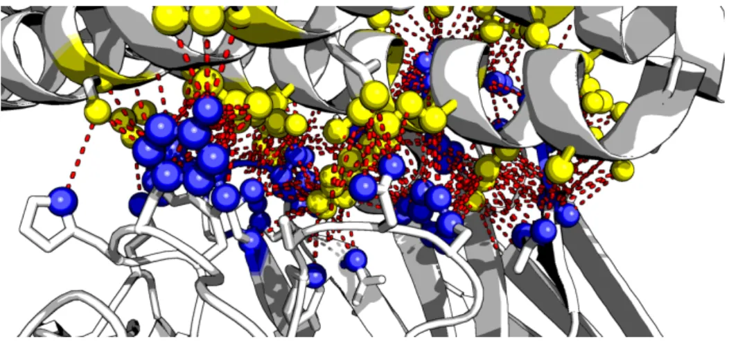
Protein-protein interactions (PPIs) are understood as physical contacts between proteins that occur in a cell or in a living organism in vivo. These physical contacts of high specificity are established between two or more protein molecules as a result of biochemical events steered by electrostatic forces including the hydrophobic effect (Figure 2.3). Indubitably, identifica-tion of other types of protein interacidentifica-tions (protein–DNA, protein–RNA, protein–cofactor, or protein–ligand) is also crucial for a comprehensive study of the interactome [36], but these types of data should not be mixed or confused with physical PPI data.

(27)

2.2 Protein-protein interaction 13

Fig. 2.3Physical contact between two proteins. The physical PPI is the biochemical events steered by electrostatic forces (red dotted lines) between the molecules of two proteins (blue spheres and yellow spheres). Figure is reprinted from Jimwoo Leem.

2.2.1 Types of protein-protein interactions

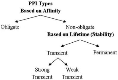
PPIs are fundamentally characterized as stable or transient, and both types of interactions can be either strong or weak (see Figure 2.4). Stable interactions are those associated with proteins that are purified as multi-subunit complexes, and the subunits of these complexes can be identical or different [37]. Transient PPIs are expected to control the majority of cellular processes. As the name implies, transient interactions are temporary in nature and typically require a set of conditions that promote the interaction, such as phosphorylation, conformational changes or localization to discrete areas of the cell. While in contact with their binding partners, transiently interacting proteins are involved in a wide range of cellular processes, including protein modification, transport, folding, signaling, apoptosis and cell cycling [37].

2.2.2 Databases for protein-protein interactions

The repositories and databases for PPI data can be broadly classified into two types based on the content: i) Those containing interactions supported by experimental evidence, and, ii) those containing interactions derived from in silico predictions alone, or, mixed with experi-mentally derived PPIs. Some of the primary databases that exclusively contain experiexperi-mentally derived PPI data in humans are listed here. They are Human Protein Reference Database (HPRD) [39], Reactome Knowledgebase [40], Alliance For Cellular Signaling (AfCS), DIP [41], IntAct [42], BioGRID [43],and MINT [44]. The last four are the core founders of IMEx, the international consortium of molecular interaction (MI) database providers [45]. This consortium, together with HUPO Proteomics Standards Initiative (PSI), has defined the

(28)

Fig. 2.4Relation of types based on affinity and stability. Non-obligate interactions are transient but there are some examples of permanent non-obligate interactions such as enzyme-inhibitor interactions. Figure reprinted from Acuner Ozbabacan et al. [38].

standard MIMIx (minimal information about a molecular interaction), which is proposed to improve data quality and curation of MIs [46].

2.2.3 Reliability of PPI data

Owing to technological advances, it has become increasingly feasible to detect large-scale PPI data experimentally. However, it is important to emphasize the limitations of available PPI data. Our current knowledge of the interactome is both incomplete and noisy. PPI detection methods have limitations as to how many truly physiological interactions they can detect and they all find false positives and negatives. With the accumulation of PPIs, more and more studies show the existence of a considerable amount of redundant data and false positive PPI data in the databases [47].

Because of the diversity of techniques for experimental detection, computational predic-tion and curapredic-tion of PPI data, adequate quality assessment methods have to account for the different evidence associated with each reported interaction. An interaction of two proteins can be supported, for example, by a single concurrent mention in a scientific publication or by multiple independent experimental observations, including details such as the protein binding interface or assay parameters [48].

MINT was one of the first PPI databases to associate to each interaction a score estimating the reliability of the interaction, given the available experimental evidence [44]. The MINT score is based on a heuristic integration of the available evidence into a ‘combined experimen-tal evidence’xwhich is then mapped in the[0,1]interval via the formulaScore=1−a−x. x

(29)

2.2 Protein-protein interaction 15

(a)Undirected graph (b)Directed graph

Fig. 2.5Example of simple graphs.

is computed by adding up all the evidence according to the formula

x=

_∑

i

d_ie_i+ n

10 (2.1)

whered reflects the size of the experiment. Experiments are defined on the large scale if the article reporting them reports more than 50 interactions otherwise they are defined on a small scale. This coefficient is set to 1 for small-scale and 0.5 for large-scale experiments.

edepends on the type of experiment supporting the interaction and emphasizes evidence of direct interaction (e=1) concerning experimental support that does not provide obvious evidence of direct interaction, i.e. Co-Immunoprecipitation (Co-IP), Pull-Down Assay, etc. (e=0.5). x takes into account the number of different publications (n) supporting the interaction [49].

The MINT scoring function assigns a score close to 1 only to interactions supported by many different reports and experimental approaches while an interaction supported, for instance, by a single high throughput pull-down experiment will receive a score of 0.2.

2.2.4 Protein-protein interaction network

Protein-protein interaction networks are the networks of protein complexes formed by biochemical events and electrostatic forces that serve a distinct biological function as a complex. The protein interactome describes the full repertoire of a biological system’s PPIs. In several PPI repositories, it is a straightforward process to obtain all the proteins that interact with a given query protein and from those to build a corresponding network of molecular interactions [50, 49]. Several bioinformatic tools have been developed to represent and explore such PPINs including Cytoscape [51], CELLmicrocosmos [52], VANESA [53] and many more tools are summarized in Pavlopoulos et al. [54].

(30)

2.3 Basic concepts in graph theory

Graph A simple graphGconsists of a nonempty setV, called the vertices (nodes) ofG, and a setE of two-element subsets ofV. The members ofE are called the edges (arcs) of

G, and the graph can be written as G= (V,E). The vertices correspond to the circles in Figure 2.5, and the edges correspond to the lines. A graph consists of vertices connected by edges. The two main categories of graphs are undirected graphs that edges do not have any particular direction (see Figure 2.5a), and directed graphs (see Figure 2.5b), where edges have direction - for example, there may be an edge from nodeAto nodeB, but no edge from nodeBto nodeA.

Graphs can be represented as a two-dimensional boolean adjacency matrix, in which the rows and columns are the sources and destination vertices, and entries in the array indicate whether an edge exists between the vertices, as in below:

Adjacent MatrixA=      0 1 1 0 1 0 1 1 1 1 0 1 0 1 1 0     

where a non-zero value atA_{i j} indicates that nodeiis connected to node j.

Distance The distance between two vertices in a graph is the number of edges on the shortest path between them. In Figure 2.5, the distance fromAtoEis 2, whereas it is 1 from

AtoC.

2.4 Gene co-expression network analysis

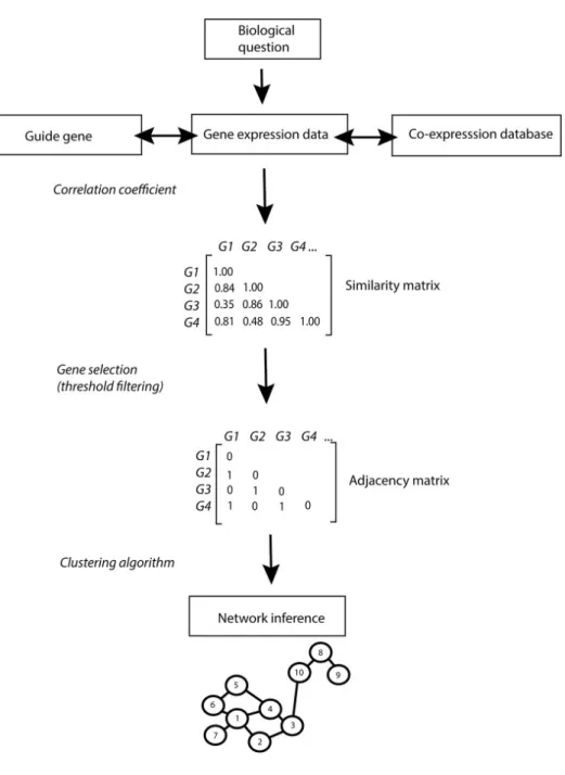
Gene co-expression network analysis (GCNA) is a popular approach to analyze a collection of gene expression profiles. GCNA yields an assignment of genes to gene co-expression modules, a list of gene sets statistically over-represented in these modules, and a gene-to-gene network. Figure 2.6 shows the pipeline of construction of gene co-expression network. Constructing a network of genes from expression data generally consists of the following steps: 1. Prior knowledge can be used to identify guide-genes, and co-expression databases can be queried to investigate gene co-expression patterns across multiple conditions. 2. Similarity in gene expression patterns is calculated using correlation coefficients (e.g. Pearson, Spearman). A user-defined threshold (in this example set at 0.8) enables the selection of genes with high co-expression scores. Significantly co-expressed genes are reported in the binary adjacency matrix as 1. 3. A clustering algorithm is applied on the adjacency matrix to

(31)

2.5 Bayesian inference and Gibbs sampling 17

infer networks of significantly co-expressed genes. In the resulting network, significantly co-expressed genes are depicted as numbered vertices linked by edges. A widely used approach to attach biological meaning to modules is to determine functional enrichment among the genes within a module using GCNA tools. Assuming that co-expressed gene are functionally related, enriched functions can be assigned to poorly annotated genes within the same co-expression module, and an approach commonly referred to as ’guilt by association’ (GBA). GBA approaches are also widely used to identify tissue or cell type specific genes if a substantial proportion of the genes within a module are associated with a particular tissue or cell type, such as the tissue-specific interaction network database, GIANT [10].

2.5 Bayesian inference and Gibbs sampling

The Bayesian interpretation of probability is one of two broad categories of interpretations. Bayesian inference updates knowledge about unknowns, parameters, with information from data. The basis for Bayesian inference is derived from Bayes’ theorem.

p(θ |y) = p(y|θ)·p(θ)

p(y) (2.2)

with observationsyand parameter set θ. p(y) will be discussed below, p(θ)is the set of

prior distributions of parameter setθ before y is observed. p(y|θ)is the likelihood function,

in which all variables are related in a full probability model. p(θ|y)is the joint posterior

distribution of parameter setθ that expresses uncertainty about parameter setθ after taking

both the prior and data into account. Since there are usually multiple parameters,θ represents

a set of jparameters asθ =θ1, . . .θj.

The goal of Bayesian inference is to maintain a full posterior probability distribution over a set of random variables. Sampling algorithms based on Monte Carlo Markov Chain (MCMC) techniques [56] are one possible way to maintain and use this distribution in the inference models. The underlying logic of MCMC sampling is the estimation of any desired expectation by ergodic averages. Any statistic of a posterior distribution can be computed as long asN samples are simulated from that distribution [57].

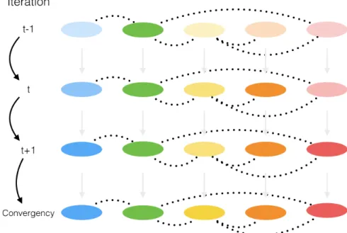
Gibbs sampling is one MCMC technique suitable for the task. The idea of Gibbs sampling is to generate posterior samples by sweeping through each variable (or block of variables) to sample from its conditional distribution with the remaining variables fixed to their current values. For instance, consider the random variablesX1,X2, andX3. We start

by setting these variables to their initial valuesx(₁0),x₂(0) andx(₃0). At iterationi, we sample

(32)

and samplex₃∼ p(X₃=x₃|X₁=x(₁i),X₂=x(₂i)). This process continues until “convergence” (the sample values have the same distribution as if they were sampled from the true posterior joint distribution). Algorithm 1 describes a generic Gibbs sampler.

Algorithm 1:Gibbs sampler

1 Initializex(0)∼x(₁0),x(₂0), . . . ,x(_D0). foriteration i=1,2, . . . do 2 x(₁i)∼p(X₁=x₁|X₂=x₂(i−1),X₃=x₃(i−1), . . . ,X_D=x(_Di−1)) x(₂i)∼p(X₂=x₂|X₁=x₁(i),X₃=x(₃i), . . . ,X_D=x(_Di−1)) .. . x(_Di)∼p(X_D=x_D|X₁=x(₁i),X₂=x(₂i), . . . ,X_D₋₁=x(_Di)₋₁) 3 end

In Algorithm 1, the posterior distribution is sampled by sweeping through all the posterior conditionals, one random variable at a time. The samples simulated based on this algorithm at early iterations may not necessarily be representative of the actual posterior distribution due to the initialization with random values. However, the theory of MCMC guarantees that the stationary distribution of the samples generated under Algorithm 1 is the target joint posterior. For this reason, MCMC algorithms are typically run for a large number of iterations (in the hope that convergence to the target posterior will be achieved). Because samples from the early iterations are not from the target posterior, it is common to discard these samples. The discarded iterations are often referred to as the “burn-in” period [58].

2.6 Markov random field

A MRF is an probabilistic graphical model that efficiently represents the joint probability distribution of a set of random variables by encoding dependencies between them. Such dependencies can be learned from data or derived from prior knowledge about the domain which is modeled. Unlike a standard classifier, an MRF enables collective inference over the entire set of known and unknown variables. MRF models have been widely used in image analysis in order to account for the local dependency of the observed pixel intensities [59]. It was also used to solve issues in system biology such as identification of differentially expressed genes [60], protein function prediction [61] involve the solution of a probability distribution defined by a discrete MRF. The concept of MRF model which is helpful for understand this thesis is briefly introduced in below. More detailed knowledge on MRF and probabilistic graphical model can be found in Koller and Friedman [62].

(33)

2.7 Multi-label dataset and classification 19

MRF is a undirected graph model of a joint probability distribution. It consists of an undirected graphG= (ν,ε). Consider all the nodes on graph as a set of random variablesX= X1,X2, . . . ,Xn, where each variableXi∈Xtakes a value from the label setL=l1,l2, . . . ,lk.

A labelingxrefers to any possible assignment of labels to the random variables and takes values from the setLn_{. The label set corresponds to segments in the case of the segmentation}

problem and protein function in case of the protein function prediction problem. The corresponding Gibbs energy function E: Ln_−→

R maps any labeling x∈Ln to

a real number E(x) called its energy. Energy function are the negative logarithm of the posterior probability distribution of the labeling. Maximizing the posterior probability equals to minimizing the energy function and leads to the maximum likelihood estimation (MLE) or maximum a posteriori (MAP) solution.

The unary potential φ(xi) represents the cost of the assignment: Xi =xi , while the

pairwise potentialφi j(xi,xj)represents that of the assignment: Xi=xiandXj=xj. Energy

functions can be decomposed into sum over unary(φi) and pairwise(φi j) potentials as:

E(x) =

_∑

i∈V

φi(xi) +

∑

(i,j)∈E

φi j(xi,xj) (2.3)

whereν is the set of all random variables (the nodes onG) andε is the set of all pairs of

interacting variables (the edges onG). Furthermore, the potential functions could be with three or more variables [63].

2.7 Multi-label dataset and classification

In many application domains each data sample is associated with a set of labels, instead of only one class label as in traditional classification. Therefore, with Y being the total set of labels in an multi-labeled dataset (MLD) Dand x_i a sample in dataset D, a multi-label classifier must produce as output a set Z_i⊆Y with the predicted labels for the i-th sample. As each distinct label in Y could appear inZ_i, the total number of potential different combinations would be 2|Y|. Each one of these combinations is called a label set. The same label set can appear in several instances ofD.

Imbalance of dataset In binary classification, the imbalance level is measured taking into account only two classes: the majority class and the minority class. For an imbalanced MLD, meaning that some of the labels are very frequent whereas others are quite rare, the level of imbalance of a determinate label can be measured by the imbalance ratio, IRLbl, defined in Equation (2.4). To know how imbalance is datasetD, the MeanIR measure is calculated

(34)

as the mean imbalance ratio among all labels, as shown in Equation (2.5). To know the significance of this last measure, the standard CV (Coefficient of Variation, Section 2.7) can be used. The SCUMBLE measure in Section 2.7 aims to quantify the imbalance variance among the labels present in each data sample [64].

IRLbl(y) = arg max y′∈L ∑|_iD₌|₁h(y′,Yi) ∑|_iD₌|₁h(y,Yi) (2.4) MeanIR= 1 |L|_y

∑

_∈_L(IRLbl(y)) (2.5) CV IR= IRLblσ MeanIR (2.6) IRLblσ = v u u t Y|Y|

∑

y=Y1 (IRLbl(y)−MeanIR)2 |Y| −1 (2.7) SCU MBLE(D) = 1 |D| |D|

∑

i=1 [1− 1 IRLbl_i( |L|

∏

l=1 IRLbl_il)(1/|L|)] (2.8) This characteristic makes this task even more challenging. Generally, the imbalance problem has been faced with three different approaches: data re-sampling, algorithmic adaptations, and cost-sensitive classification [65].

2.8 Text mining data curation

Text mining is also known as knowledge discovery in text data mining. It is the process of extracting previously unknown, understandable, potential and practical patterns or knowledge from a collection of massive and unstructured text data. It is a combining technique from data mining, machine learning, natural language processing, information retrieval, and knowledge management [66, 67]. Numerous text mining techniques and tools were applied in life science, e.g. mapping of genes diseases and drug discovery [68, 69], in social media, e.g. recommendation system on Facebook and Twitter [70], business intelligence, e.g. analysis of the customer satisfaction [71].

(35)

2.8 Text mining data curation 21

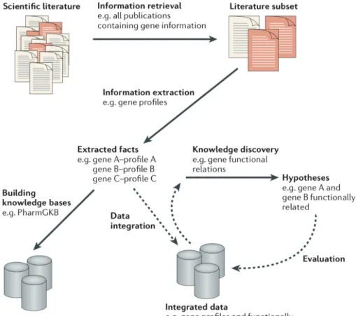
A generic overview of text mining process is illustrated in Figure 2.7 which was sum-marized by Rebholz-Schuhmann et al. [68]. The larger text-analytical approaches typically include:

1. Information retrieval. The tasks include data selection, document retrieval, classifica-tion, and feature extraction generally convert the documents into intermediate forms, which should be suitable for different mining purpose.

2. Information extraction from the text and are the central part of a text mining system. Information extraction comprises the identification of entities, such as genes or diseases, as well as the identification of complex relationships between those entities, including protein-protein interactions and gene-disease associations by using the algorithms including clustering, association rule discovery, trend analysis, pattern discovery and other knowledge discovery algorithms.

3. Post-processing. These tasks manipulate data or knowledge coming from information extraction step. These scientific facts can then either be used to populate databases directly or to assist the work of curation teams including the evaluation and selection of knowledge, interpretation, and visualization of knowledge. The text mining results are used to suggest hypotheses that can then be used to shape or to plan experiments to validate or to disprove the proposed hypotheses.

(36)

.

Fig. 2.6Co-expression network inference pipeline. Figure reprinted from Serin et al. [55]

(37)

2.8 Text mining data curation 23

Fig. 2.7Pipeline of text mining solution. Figure reprinted from Rebholz-Schuhmann et al. [68].

(38)

(39)

Chapter 3 Overview of protein subcellular

localization prediction

Understanding of the SCLs of proteins has always been an essential aspect to discover the novel function of the protein, the primary mechanisms of the cell. We are interested in where is a protein localized in the cell? How is a MLP distributed in the cell simultaneously, or exclusively? How does the protein move from one SCC to another? Under which biological context the translocalization of protein is induced? Furthermore, how is the protein interacting with the other molecules in the cell? How to collect and access this SCL data? How to analyze the SCL data? How to interpret them along with protein functions? In this chapter, we discuss the current situation of protein SCL analysis and prediction.

3.1 Access to the protein SCL data

3.1.1 Experimental data

Conventional wet-lab experiments are used to access the SCL of proteins and also as the gold standard for validating SCL. Several wet-lab approaches for systematic analysis of protein SCLs have been developed.

• Initial research was done with specific staining and light microscopy. Closer scrutiny of micrometer- and nanometer-sized subcellular structures was later enabled by the rise of electron microscopy, which illuminated the complexity of organelles and their various positions within the cell [72].

• Quantitative mass-spectrometric readouts allow identification of proteins with simi-lar distribution profiles across fractionation gradients [73–75] or enzyme-mediated

(40)

proximity-labeled proteins in cells [75–77]. These techniques make it possible to understand what is each component doing at the molecular level.

• Imaging-based approaches enable the exploration of the subcellular distribution of proteins in situ in a single cell and have the advantage of also effectively identifying single-cell variability and multi-organelle localization. Imaging-based approaches can be performed using tagged proteins [78] or affinity reagents [28]. Such as the immunofluorescence (IF) based approach can be combined with confocal microscopy was utilized to perform the high-resolution investigation of the spatial distribution of each protein.

Finally, genetics, in all its forms, has allowed us to dissect the structure and function of these SCLs by selective disruption of individual cell components. These experimental data can be retrieved from databases such as Human Protein Atlas (HPA) [28], LocDB [79] and ENCODE [80].

3.1.2 Knowledge-bases of protein SCLs

However, not all the experimental data are collected and accessible in databases. A vast amount of data are spread over the scientific research for various purposes. Such data re-quire to be integrated, interpreted, standardized and enriched from literature and numerous resources to a knowledge base. UniProt Knowledgebase (UniProtKB) leads the world in providing full and comprehensive curation of the experimental data in the literature and does this in a mutually beneficial collaboration with other specialized resources. Literature-based expert curation of UniProtKB provides high-quality information for experimentally characterized proteins in a standardized and structured way using widely accepted con-trolled vocabularies and ontologies. Other knowledgebases of protein SCL include the Reactome Knowledgebase [40], Human Protein Reference Database [81] and Gene Ontology annotations [82].

3.1.3 Limitations

Experimentally determining the SCLs of a protein can be a laborious, expensive and time-consuming task, and manually annotating a protein, particularly identifying the massive SCL data from heterogeneous sources, is always a challenging and low-throughput task.

(41)

3.2 Computational prediction method 27

3.2 Computational prediction method

Over the last decades, a variety of computational methods have been developed for predicting the SCL of proteins for various organisms [83, 84], which allows us to tackle the exponentially growing number of ’omics’ data and access the protein SCL data in a large scale. Predicted localization data, in particular, offer numerous insights that can assist in the prioritization of proteins for downstream analysis. Because localization and function depend on each other, a protein’s localization can provide clues to its role in the cell when other information is not available.

3.2.1 Sequence feature based methods

With the rapid growth in publicly available sequence data, the computational prediction of such sequence features has become an essential aspect of biological research. By computa-tionally identifying one or more of the signals that are known to influence protein targeting, or sequence features that correlate with a specific SCL, a protein’s probable SCL can be deduced automatically using protein sequence information. These predictors utilized various methods which can be categorized into the following types:

Homology-based methodscompare the SCLs of known proteins with unknown proteins. If a certain degree of similarity is found in the sequence, then it can be inferred that the unknown protein’s SCL may be the same as the known protein, such as SCLpredT [85] and GOASVM [86].

Sorting-signal-based methodsare more specific which recognizes the signal peptides which are responsible for protein translocation [87]. Most of the signal-based predictors aim to predict only one particular SCL, such as NucPred [88] and ChloroP [89].

Composition-based methods depend on information about the primary amino acid sequence of proteins used for information technology operations or discovery of hidden information, commonly including amino acid composition [90, 91], pseudo amino acid composition [92–94], andn-gram [95, 96]. Prediction results from this approach are typically less informative than those for homology- and functional domain-based methods, but in predicting SCL of unknown proteins, it is still a feasible approach.

Functional domain-based methodsrely on known structures or functional data, such as protein functional domains [97–99] and motifs [100, 101], as well as information in the GO database [97, 102]. There are many learning models of research methods are used to establish the relevance of GO terms and SCL. It has been shown that GO terms can be used to advance the performance of SCL prediction. These functional data regarded as domain knowledge are highly accurate and reliable, but this approach requires manual verification of

(42)

each annotation and cannot be applied to the entirely new protein. Therefore it is usually combined with the homology-based approach [103].

Combined methods, as the name implies, these methods combine the above-mentioned protein sequence features [97, 104]. Zhou et al. incorporate multiple features, such as context vocabulary annotation-based GO terms, peptide-based functional domains, and residue-based statistical features, and use a hidden correlation modeling as a feature representation protocol which creates more compact and discriminative feature vectors by modeling the hidden correlations between annotation terms. Briesemeister et al. presented an algorithm YLoc which is based on the simple, naive Bayes classifier. They selected up to 30 most significant features from about 30 000 features from protein sequences including sorting signal, amino acid composition, and pseudo composition as well as properties such as hydrophobicity, charge, and volume of amino acids. Also, they included PROSITE motifs [105] and GO terms from close homologs. Another remarkable advantage of YLoc is that YLoc provides the details of how a prediction was made and which biological property and features of the protein was mainly responsible for it [104], whereas most of SCL prediction tools are designed as ’black box’ from which the results are hard to interpret.

3.2.2 Protein-protein interaction network-based approaches

Many biological processes are mediated by dynamic interactions between proteins. Two proteins can interact with each other only if they co-occur spatially and temporally. As PPI and SCL are often discovered via separate empirical approaches, the annotations of PPI and SCL are independent and might complement each other in helping us to understand the role of individual proteins in cellular networks. We expect reliable PPI annotations to show that proteins interacting in vivo are co-localized in the same SCC.

Many studies based on high-throughput technologies have confirmed that interacting proteins tend to be localized within the same SCC, or in the physically adjacent SCCs, in various types of species. [106] reported that 76% of interactions in their yeast PPI set are localized in the same SCL, whereas a review of human PPIs based on public databases and literature curation found 52% to involve co-localized proteins plus others involving adjacent SCC [107]. These studies strengthen the assertion that a pair of interacting proteins is more likely to be co-localized in the eukaryotic cell.

The existing protein-protein interaction network (PPIN)-based methods of protein SCL prediction can be classified into three categories.

(43)

3.2 Computational prediction method 29

Neighborhood counting & probabilistic methods

Neighborhood counting-based approach proposed by Shin et al. [21] is the most straightfor-ward algorithm that determines the SCL of a protein based on the known SCL of proteins lying in its neighborhood. One of the variants is the majority method, which takes the most annotated SCL terms as the prediction result. In the merged variant, for each protein, a SCL is assigned based on the union of annotations for all its interaction partners. In contrast, for the common variant method, when a protein interacts with more than one other protein only those SCL common to all its interaction partners are employed as a prediction.

Lee et al. [108] explore protein features in combination with PPINs to predict the SCLs for unknown proteins (i.e. the proteins which have no SCL information). They consider the impact of not only direct interacting neighbors but also all proteins at network distances up to five and including distance (see Section 2.3). They generated a weighted network feature vector based on each neighbor’s significance and the conditional probabilities of interactions between localization pairs. Afterward, a model of SCL selection was constructed by using the supervised learning methodknearest neighbor (kNN) classifier based on both the protein feature dataset and the localization-interaction dataset to support the prediction of an unknown protein.

Du and Wang propose to use PPIN as an infrastructure integrated with the existing sequence-based predictors (Hum-mPloc 2.0 [110], Y-Loc [111]). They calculate the prob-ability based on the neighbor protein’s SCL annotation and the membership degree (see Section 2.3) of a protein in a probable SCC. In their approach, the topology of the PPIN is taken into account. Edge clustering coefficient (ECC) was firstly used for the selection of essential nodes in the context of a PPI network and was proven to be a potential indicator to whether two interacting proteins tend to have common SCC [109].

Graph theory methods

As a PPIN can be considered as a graph G= (V,E) in which the nodesV represent the proteins and the edgesE serve as the PPIs. The nodesV are associated with the variables

X which stand for the probable SCLs label of proteins. Hence, it is natural to apply graph algorithms for the SCL assignment problem.

In contrast to the local neighborhood counting methods, the graph-based approaches are global and consider the full topology of the network. Jiang and Wu [112] applied different graph-based semi-supervised learning algorithms to assign SCL to proteins. These algorithms include χ2-score, GenMultiCut, and Functional Flow which are initially used

(44)

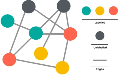
Labelled

Unlabelled

Edges

Fig. 3.1Protein-protein interaction network as an undirected graph.The nodes represent the proteins and the edges represent the PPIs. The colors of the nodes serve as the available SCL label of proteins. Grey color indicates that the SCL information is unknown for this protein.

χ2-score algorithm to determine the over-represented SCL from all available annotated SCL

information of the neighborhood ofxwith a distance up to three. Whereas the GeneMultiCut algorithm [114] utilizes a cut-based methodology to maximize the number of times the same SCL annotations are associated with neighboring proteins. The task is to partition a graph in a way that each ofknodes belongs to a different subset of the partition to assign a unique SCL to all the unannotated nodes. The assignment is made by minimizing the sum of the costs (which is defined in their score function) of interacting nodes with no SCL in common.

Besides, a flow-based algorithm that simulates functional flow between proteins is applied to predict protein SCL. The proteins which the SCL information are known are treated as a ‘source’ of ‘functional flow’. After simulating the spread of this functional flow through the neighborhoods surrounding the sources, each protein in the neighborhood is assigned with a score. This score corresponds to the amount of ‘flow’ that the protein has received for that function, over the course of the simulation which determines the SCL of the protein.

Methods which integrates multiple information sources

Moreover, several authors have extended the PPI data by integrating different data sources for SCL prediction. Mintz-Oron et al. [115] introduced a constraint-based method for predicting SCL of enzymes based on the embedding metabolic network, relying on a parsimony principle of a minimal number of cross-membrane metabolite transporters.

Context-specific subcellular localization prediction: Leveraging protein interaction networks and scientific texts