An innovative feature selection method for support vector machines and its test on the estimation of the credit risk of default

(1)

Rev Financ Econ. 2018;1–24. wileyonlinelibrary.com/journal/rfe

|

1

1 | INTRODUCTION

The introduction of the Basel III guidelines (BCBS, 2001) and the new capital requirements that banks must meet have estab-lished the necessity of an accurate risk assessment. The probability of default (PD) measure is a key estimate not only for risk assessment, but also for impairment purposes under the changes introduced by International Financial Reporting Standard 9 (IFRS9) (Onali & Ginesti, 2014). Accurate PD assessment is vital for decreasing the cost of capital (Gavalas, 2015). The esti-mation of the PD has been a topic of extensive research for many years. A high number of different algorithms have been used to estimate the PD: artificial neural networks (ANN), decision trees (DT), linear discriminant analysis (LDA), support vector machines (SVM), logistic regression (LR). Harris (2015) provides a good general explanation of these methods. However, LR remains the most widely used PD estimation method for both corporate and retail borrowers.

Extensive research has been conducted comparing several PD estimation methods. Meyer, Leisch, and Hornik (2003) com-pared SVM to 25 other methods used for PD estimation. They found that although the performance of the SVM model is good, other methods such as ANN and DT sometimes outperform SVM. In a more general study, Mukherjee (2003) used SVM and LR to classify traded companies on the Greek stock exchange, showing that SVM classification was better, still without focus

O R I G I N A L A R T I C L E

An innovative feature selection method for support vector

machines and its test on the estimation of the credit risk of default

Eduard Sariev

|

Guido Germano

Department of Computer

Science, University College London, London, UK

Correspondence

Eduard Sariev, Department of Computer Science, University College London, London, UK.

Email: [email protected] Funding information

Economic and Social Research Council (ESRC), Grant/Award Number: ES/ K002309/1

Abstract

Support vector machines (SVM) have been extensively used for classification problems in many areas such as gene, text and image recognition. However, SVM have been rarely used to estimate the probability of default (PD) in credit risk. In this paper, we advocate the application of SVM, rather than the popular logistic regression (LR) method, for the estimation of both corporate and retail PD. Our results indicate that most of the time SVM outperforms LR in terms of classification accuracy for the corporate and retail segments. We propose a new wrapper feature selection based on maximizing the distance of the support vectors from the separating hyperplane and apply it to iden-tify the main PD drivers. We used three datasets to test the PD estimation, containing (1) retail obligors from Germany, (2) corporate obligors from Eastern Europe, and (3) cor-porate obligors from Poland. Total assets, total liabilities, and sales are identified as frequent default drivers for the corporate datasets, whereas current account status and duration of the current account are frequent default drivers for the retail dataset.

J E L C L A S S I F I C A T I O N C10, C13

K E Y W O R D S

default risk, logistic regression, support vector machines

This is an open access article under the terms of the Creative Commons Attribution License, which permits use, distribution and reproduction in any medium, provided the original work is properly cited.

(2)

on the feature selection process. Another comparison between SVM and ANN was made by (Li, Shiue, & Huang, 2006). They showed that the SVM model slightly outperforms ANN and the SVM model needs fewer features than ANN to achieve maxi-mum classification performance. Huang, Chen, and Wang (2007) compared SVM with ANN, genetic programming, and DT. In this comparison, the feature selection process was covered, but the LR model was not used as a comparison. Bellotti and Crook (2009) compared LR and SVM, but without showing the feature selection method for the LR. Bellotti, Matousek, and Stewarti (2011) compared LR with SVM, but for regression purposes, not for classification. They found that the SVM model outper-forms LR. Furthermore, Chen, Härdle, and Moro (2011) compared LR and SVM with regard to the feature selection process. However, the features selected for the SVM were automatically used for LR and this way the comparison was biased toward the SVM model: as expected, the SVM model outperformed the LR in this case. Hens and Tiwari (2012) again focused on the comparison of SVM with genetic programming without including LR. Lessmann, Baesens, Seow, and Thomas (2015) found that SVM and ANN perform better, but the performance of the LR is still relatively good. Finally, Harris (2015) compared SVM to LR. Although this study used LR as the only alternative to SVM, a lot of the details of this comparison were not shared; for instance, the feature selection for both models is not covered at all.

The feature selection process for SVM is a key step in comparing SVM to other algorithms. The existing literature indicates that some research on SVM feature selection has been developing recently. Weston et al. (2000) proposed a method that is based upon finding those features which minimize bounds on the leave-one-out error. They show that their method is superior to some standard feature selection algorithms. Guyon and Elisseeff (2003) provided a good high-level overview of the different feature selection algorithms available in the literature. Rakotomamonjy (2003) proposed relevance criteria derived from SVM that are based on a weight vector. He showed that the criterion based on the weight vector derivative achieves good results and performs consistently well. Chen and Lin (2006) combined SVM and various feature selection strategies. Some of them were filter-type approaches, i.e., general feature selection methods independent of the SVM, and some were wrapper-type methods, i.e., modifications of the SVM which can be used to select features. Recently, variable and feature selection has become the focus of much research. Becker, Werft, Toedt, Lichter, and Benner (2009) investigated a penalized version of SVM for feature

selection. They argued that keeping a high number of features could avoid overfitting if the performance function uses an L₁

norm regularization. Huang and Huang (2010) investigated a recursive feature selection scheme in SVM. Their results have indicated that one-vs.-one SVM with embedded recursive feature selection outperforms other multiclass SVM. In this context, Kuhn and Johnson (2013) presented a generalized backward feature elimination procedure for selecting a final combination of features.

With respect to the above discussed articles on feature selection for SVM, this article contributes to the literature firstly by proposing an innovative feature selection for SVM and LR. Secondly by showing that most of the time the SVM model renders higher classification accuracy than logistic regression.

The rest of the article is organized as follows. Section 2 presents the theoretical formulation of SVM. Section 3 contains an empirical analysis, including the presentation of the data and the obtained results. Section 4 discusses the business rationale of the selected default drivers. Finally, section 5 concludes the paper, summarizes the main findings of this research, and proposes some future research directions.

2 | THEORETICAL FOUNDATIONS

2.1 | Support vector machines

Consider a dataset of n pairs A= {(x_i, y_i)|x_i_∈_ℝp_{, y}

i∈ {−1,+1}}n_i=1, where xi is a p-dimensional “feature” vector and yi is a label, i.e., a categorical variable whose value gives the class to which x

i belongs. Provided the data are linearly separable, SVM build a hyperplane that separates the points with y_i= +1 from those with y_i= −1 maximizing the margin M, i.e., the

Highlights

1. We estimate the probability of default on credit risk data for corporate and retail clients. 2. We compare support vector machines (SVM) and logistic regression (LR).

3. The SVM model often outperforms LR in terms of classification accuracy.

4. We propose and test a new variable selection method designed specifically for SVM. 5. We identify important default drivers and analyse them.

(3)

minimum distance between the hyperplane and each point; the width of the separating band is thus 2M. For this reason, SVM are also known as maximum margin binary classifiers. A hyperplane can be written as the set of points x satisfying the implicit equation

where ŵ ₌w∕‖w‖=w∕w is a unit vector normal to the hyperplane, · is the scalar product and b/w is the distance between the

hyperplane and the origin. Thus the objective is

This optimization problem can more conveniently be rephrased as (Kuhn & Johnson, 2013)

where M=1/w, and the distance of the hyperplane from the origin is b/w (Boser, Guyon, & Vapnik, 1992). Mathematically it is more convenient to reformulate this as a quadratic optimization problem:

where 𝛼i are Lagrange multipliers. The solution 𝜶∗ determines the parameters w∗ and b∗ of the optimal hyperplane for the dual

optimization problem. Usually, only a small number of Lagrange multipliers are positive and the corresponding vectors are in the proximity of the optimal hyperplane. The training vectors x_i corresponding to the positive Lagrange multipliers are called

support vectors.

An extension of the above concept can be found in the nonseparable case (Cortes & Vapnik, 1995). The problem of finding the optimal hyperplane has the expression

where ξ is a positive “slack” variable and C is a user-defined penalty parameter. The optimization problem in Equation (5)

can be solved with the Lagrangian method Rockafellar (1993) as before, except that now 0≤𝛼_i≤C.

Nonlinear SVM map the training samples from the input space to a higher-dimensional feature space via a function 𝚽(x_i₎

(Cristianini & Shawe-Taylor, 2000). The use of a kernel function avoids to specify an explicit mapping:

Many kernel functions have been investigated in the literature. One of the most useful Broomhead and Lowe (1988) is a radial basis function (RBF),

where 𝛾 =1∕𝜎2 is the scaling parameter. The kernel generalization of the decision function for each _x i is

where n is the number of instances, k_i(x_,x_i₎ is element i of the output vector k₍x_,x_i₎, and x is the feature matrix.

One of the less investigated areas of SVM is the width of the hyperplane that separates the labels (Chang & Lin, 2011). The average distance of the support vectors from the hyperplane is called hyperplane width:

(1) ̂ w_⋅x₋b=0, (2) max ̂ w_,b M subject to yi(̂ w_⋅x_i_−b₎≥1 for 1≤i≤n. (3) min w_,b w subject to yi(w⋅xi−b)≥1 for 1≤i≤n, (4) arg max � n ∑ i=1 𝛼_i−1 2 n ∑ i=1 n ∑ j=1 𝛼_i𝛼_jyiyjxi⋅xj �

subject to 0≤𝛼_i for 1≤i≤n and n ∑ i=1 𝛼_iy_i=0, (5) arg minw,b,𝜉 � 1 2w 2₊_C∑n i=1𝜉i � subject to y_i(w_⋅x_i+b+ 𝜉_i−1)≥0 and 𝜉_i≥0, (6) 𝚽(x_i)_⋅_𝚽(x_j)₌k(x_i, x_j). (7) k(x_i_,x_j₎₌_exp � − 1 2𝜎2‖xi−xj‖ 2 � (8)

=exp (− 𝛾x2_i) exp (− 𝛾x_j2) exp (2𝛾x_i_⋅x_j_),

(9) f(x,𝜶 ∗,b∗)=sgn ( n ∑ i=1 𝛼_iy_ik_i(x,x_i)₊b ) , (10) ̄ D=1 s s ∑ l=1 D_l.

(4)

The distance D_l of support vector l from the hyperplane is

where

f(.) is a decision function and k_lm(x_,x₎ is element lm of the output matrix k(x, x).

Instead of predicting a label y_i, many applications require a posterior class probability P(yi =1|xi). The transformation of class labels to PD estimates is done with Platt’s method (Platt, 2000).

2.2 | Data transformations

The comparison of different models depends on how the data are transformed. This is another aspect that is rarely dis-cussed when model performance is assessed. From a practical point of view, data transformations play a pivotal role in every statistical model (Box & Cox, 1964). With the aim of being objective, a truncated sigmoid transformation was applied to data prior to modeling the default probabilities. The sigmoid function or logistic curve is a popular practical choice that allows to diminish the outliers’ effect and to bound the feature values between 0 and 1 (Balaji & Baskaran, 2013):

where x0 =( maxx−minx)∕2 is the midpoint and k=2.95∕( max x−x0) gives the steepness of the curve. The number 2.95

used for the estimation of the steepness and the cutoff at x₀ ±100 are subjective decisions by the statistical analyst, chosen to

ensure that the transformation will produce meaningful results.

3 | EMPIRICAL ANALYSIS

The East-European dataset contains 7,996 observations on 33 independent variables (covariates or features) and on one binary target variable, which shows whether a default occurred one year after the issue of the financial statement. The 33 covariates were constructed based on data from the entity’s financial statements. These financial ratios were split into several groups and further analysed. The data are on an annual basis from the period 2007–2012. The dataset is not publicly available, but the authors can share the dataset if requested.

The Polish data is publicly available (Tomczak, 2016). The data were collected from Emerging Markets Information Service, which is a database containing information on emerging markets around the world. The bankrupt companies were analyzed from 2000 to 2012, while the still operating companies were evaluated from 2007 to 2013. The data set has 5,910 observations on 64 independent variables. The default indicator shows the bankruptcy status after one year.

Before modeling the one year corporate PD, two main actions were taken on the data:

1. Missing values analyses. As it usually happens, the financial statements contain missing values. In order to tackle this problem, a detailed analysis is performed on the missing patterns in the data and finally a multiple chain imputation method (Abayomi, Gelman, & Levy, 2008) is used for the East-European data and a simple mean imputation is applied to the Polish data; see Tables A2 and A3 in Appendix A: Descriptive statistics, which present the descriptive statistics before and after imputation for both datasets. We apply a simpler imputation on the Polish data due to the lower number of missing values.

2. Outliers treatment. As it was expected, the financial statements contain outliers. In order to tackle this problem a sigmoid transformation is applied to all the covariates, thus bounding the covariates’ value between 0 and 1 (Han & Moraga, 1995). This is a typical approach applied to variables before using them for classification purposes. The Polish data are standardized, which is another popular transformation applied in classification problems.

(11) D_l=1 w|f(xl,𝜶∗,b∗)|, (12) w= √ √ √ √ s ∑ l=1 s ∑ m=1 y_ly_m𝛼_l𝛼_mk_lm(x, x), (13) f(x)= { 0 if|x−x₀|≥100 1 1+e−k(x−_x0) if|x−x0|<100,

(5)

The retail dataset contains information for 1,000 observations on 20 independent variables (covariates or features) and on one binary target variable, which shows whether a default occurred. The dataset contains categorical and numerical variables. The categorical variables are transformed on a continuous scale by mapping them to integer number corresponding to the level of each category. Thereafter, the variables (continuous and categorical) are standardized. There are no missing values in the dataset. For the feature names and construction refer to Appendix A: Descriptive statistics, Table A1. The dataset contains attributes for German credit borrowers and is freely available (Hofmann, 1994).

Figure 1a presents the box plots of the variables in the East-European corporate data. It can be seen that some variables have significantly different modes when slipted by good (nondefault) and bad (default) obligors. Figure 1b below presents the box plots of the variables in the retail data. In this data, however, most variables have the same mode when slipted by good (nondefault) and bad (default) obligors. The names of the variables are presented in Appendix A: Descriptive statistics.

Figure 2a,b presents the box plots of the variables in the Polish corporate data.

3.1 | Feature selection

The objective of variable selection is threefold: improve the prediction performance of the predictors, provide faster and more cost-effective predictors, and provide a better understanding of the underlying process that generates the data.

The statistical literature offers many approaches for feature selection (Guyon & Elisseeff, 2003). However, there is no proven methodology that works for each dataset. Based on previous experience on the selection of appropriate features for different models, we decided that an automatic script shall be written that overcomes many of the drawbacks of a manual feature selection process. An univariate analysis on the features is the most common approach used for feature selection: those features that exhibit good performance based on a specific measure, for example, the F-score (Güneş, Polat, & Yosunkaya, 2010), are selected for further analysis. Nevertheless, there are some negative aspects of this approach (Quanquan, Zhenhui, & Jiawei, 2011):

1. Some variables cannot discriminate well on a standalone basis but show better explanatory power in a combination with other factors.

2. Often the modeler selects a combination of factors that is highly correlated and even though they have a strong performance on a univariate level, it is difficult to select a combination of factors with a low multicollinearity.

FIGURE 1 (a) Box plots on the variables in the East-European corporate data. (b) Box plots on the variables in the German retail data

V1 V2 V3 V4 V5 V6 V7 V8 V9 V10 V11 V12 V13 V14 V15 V16 V17 V18 V19 V20 −1.0 −0.5 0.0 0.5 1.0 0 2 4 −2 −1 0 1 −1 0 1 2 0 2 4 0 1 −2 −1 0 1 −1 0 1 −2 −1 0 1 2 0 1 2 3 4 −1 0 1 −1 0 1 −1 0 1 2 3 −2.5 −2.0 −1.5 −1.0 −0.5 0.0 0.5 −1 0 1 2 0 1 2 3 4 −3 −2 −1 0 1 −0.5 0.0 0.5 1.0 1.5 2.0 −0.5 0.0 0.5 1.0 0 1 2 3 4 5 V1 V2 V3 V4 V5 V6 V7 V8 V9 V10 V11 V12 V13 V14 V15 V16 V17 V18 V19 V20 variable Value def_label Bad Good V1 V2 V3 V4 V5 V6 V7 V8 V9 V10 V11 V12 V13 V14 V15 V16 V17 V18 V19 V20 V21 V22 V23 V24 V25 V26 V27 V28 V29 V30 V31 V32 V33 0.00 0.25 0.50 0.75 1.00 0.00 0.25 0.50 0.75 1.00 0.00 0.25 0.50 0.75 1.00 0.00 0.25 0.50 0.75 1.00 0.00 0.25 0.50 0.75 1.00 0.25 0.50 0.75 1.00 0.00 0.25 0.50 0.75 1.00 0.00 0.25 0.50 0.75 1.00 0.25 0.50 0.75 1.00 0.00 0.25 0.50 0.75 1.00 0.00 0.25 0.50 0.75 1.00 0.00 0.25 0.50 0.75 1.00 0.25 0.50 0.75 1.00 0.00 0.25 0.50 0.75 1.00 0.00 0.25 0.50 0.75 1.00 0.00 0.25 0.50 0.75 1.00 0.00 0.25 0.50 0.75 1.00 0.00 0.25 0.50 0.75 0.00 0.25 0.50 0.75 1.00 0.00 0.25 0.50 0.75 1.00 0.00 0.25 0.50 0.75 1.00 0.00 0.25 0.50 0.75 1.00 0.00 0.25 0.50 0.75 1.00 0.00 0.25 0.50 0.75 1.00 0.00 0.25 0.50 0.75 1.00 0.00 0.25 0.50 0.75 1.00 0.00 0.25 0.50 0.75 1.00 0.00 0.25 0.50 0.75 1.00 0.00 0.25 0.50 0.75 1.00 0.00 0.25 0.50 0.75 1.00 0.00 0.25 0.50 0.75 1.00 0.00 0.25 0.50 0.75 1.00 0.00 0.25 0.50 0.75 1.00 V1 V2 V3 V4 V5 V6 V7 V8 V9 V10 V11 V12 V13 V14 V15 V16 V17 V18 V19 V20 V21 V22 V23 V24 V25 V26 V27 V28 V29 V30 V31 V32 V33 variable Va lu e def_label Bad Good (a) (b)

(6)

In order to avoid the above drawbacks of the simpler methods for variable selection, we propose an innovative variable selection method that we apply to the three datasets described above. The applied feature selection algorithm consists of the following steps:

1. Initialization: set F = initial set of n features, D = development sample, V = validation sample and S = selected set of features, where S ⊆ F. Define fk

S = set of all feature combinations at k, where k ∈ {1, …, n} is a generation index for a

feature combination S = {i, j, …, z} with cardinality l ≤ n. Set Pk_⊆_S = final approved combinations of features for

generation k. 2. for k = 1, …, N

1. Create generation k of feature combinations Sk_{= {i}_{, j,}_…_{, z}_}_⇒_fk

S where i ≠ j ≠ ⋯ ≠ z. The number of different

feature combinations is (n r) =

n!

r!(n−r)!, where r is the cardinality of S

k and n is the total number of features. 2. For each {i, j, …, z} of generation k compute:

if model == SVM then

1. _D̄k

{i,j,…,z} = hyperplane width for f

k S. 2. sk

{i,j,…,z} = number of support vectors for f

k S. 3. AUCk_{_i_,j,_…_,z_} = area under the curve (AUC) for fk

S on V

k, where _Vk is a validation sample for a feature combination from generation k. end if if model == LR then 1. p-valuek {i,j,…,z} = a p-value for f k S

2. AICk_{_i_,j,_…_,z_} = an Akaike information criterion (AIC) for fk S 3. BICk_{_i_,j,_…_,z_} = a Bayes information criterion (BIC) for fk

S on V

k, where _Vk is a validation sample for a feature combination from generation k

end if

On Dk compute the l×l feature correlation matrix A, where l is the cardinality of {i,j,…,z}. 3. For each {i, j, …, z} of generation k, given a predefined AUC threshold AUCt test:

ifAUCk_{_i_,j,_…_,z_}≥AUCtand maximum element of A ≤ 60% then accept Pk⊆Sk for {i, j, …, z}

end if

4. Given all accepted feature combinations (Pk₎ from generation k, increase the cardinality of the set {i, j, …, z} by 1 until k = n.

end for

3. Test the performance of the model on test data on all accepted feature combinations (Pk₎ from each generation k.

if model == SVM then

1. Select the l feature combinations with the highest AUC, distance to the hyperplane and the lowest number of sup-port vectors on the test data in that order.

end if

if model == LR then

1. Select the l feature combinations with the highest AUC, AIC and BIC on the test data in that order.

end if

For the datasets under investigation, the algorithm explained above is run under the following conditions:

1. The initial number of features is equal to n, i.e., to the total number of variables in each dataset for both models. 2. The first generation k = 1 contains only two features for both models. It is assumed that including more than five

features can result in overfitting the data, especially for the logistic regression. SVM has an embedded regulariza-tion, that is, it introduces additional information in order to prevent overfitting Fan, Chang, Hsieh, Wang, and Lin (2012), but overfitting is still possible.

3. The AUC threshold in Step 2.3 is set to 60% on the validation sample.

4. The feature correlation matrix in Step 2.2 is estimated using the Pearson product-moment correlation coefficient.

5. The number of final selected feature combinations l on Step 3 of the algorithm is set to 5 for the SVM and LR. 6. To improve the computational efficiency of the algorithm, the total number of variables is reduced by randomly

sampling 10 variables out of n without replacement and running the algorithm 10 times on different random sub-samples of n.

(7)

7. The SVM model is run with an RBF kernel with parameter 𝛾 = 1

k+1. The penalty parameter C is kept constant across the

iterations and the feature combinations. This allows a direct comparison of the number of support vectors for each com-bination. The number of support vectors is also affected by the number of features in the model. However, the effect is not significant and therefore this factor is ignored when comparing the number of support vectors. The expectation is that the lower the number of support vectors the better the model. Nonetheless, we have to point out that the number of sup-port vectors is affected by several factors:

1. the size of the data (the number of observations for the validation sample and the training sample is constant for each iteration, only the content is different);

2. the cost C of constraints violation; 3. the RBF kernel.

3.2 | Selection of the best performing LR models on test data

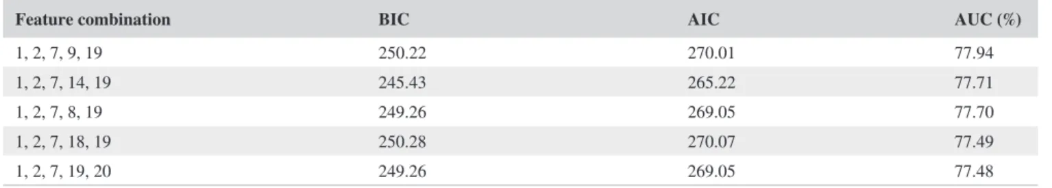
Table 1 presents the output from the feature selection method on the training data. The calibration data is split into training set and test set. The feature selection method is run on the training data and the performance is measured on the test (validation) data. The columns of Table 1 show the BIC, AIC, and AUC on the test data. The algorithm selects the five feature combinations with the lowest BIC, AIC and with the highest AUC on the test data. Tables 2 and 3 present the output of the feature selection method on the German, East-European and Polish data.

3.3 | Selection of the best performing SVM models on test data

Table 4 presents the output from the feature selection method on the training data. The calibration data are split into a training set and a test set. The feature selection method is run on the training data and the performance is measured on the test data. The col-umns of Table 4 show the distance to the hyperplane, the number of support vectors and the AUC on the test data. The algorithm selects the five feature combinations with the highest distance to the hyperplane, the lowest number of support vectors and the highest AUC on the test data. Tables 5 and 6 present the output of the feature selection method on the German, East-European, and Polish data.

FIGURE 2 (a) Box plots on the variables from 1 to 34 in the Polish corporate data. (b) Box plots on the variables from 35 to 64 in the Polish corporate data

Attr31

Attr25 Attr26 Attr27 Attr28 Attr29 Attr30

Attr31 Attr32

Attr1 Attr2 Attr3 Attr4 Attr5 0.0 Attr6

0.1 0.2 0.3 0.00 0.25 0.50 0.75 1.00 0.0 0.2 0.4 0.6 0.0 0.2 0.4 0.6 0.0 0.2 0.4 0.6 0.8 0.00 0.25 0.50 0.75 0.0 0.1 0.2 0.3 0.4 0.00 0.25 0.50 0.75 0.0 0.2 0.4 0.6 0.8 0.00 0.25 0.50 0.75 1.00 0.00 0.25 0.50 0.75 0.00 0.25 0.50 0.75 1.00 0.00 0.25 0.50 0.75 1.00 0.0 0.1 0.2 0.3 0.4 0.5 0.00 0.25 0.50 0.75 0.0 0.2 0.4 0.6 0.00 0.25 0.50 0.75 1.00 0.00 0.25 0.50 0.75 1.00 0.0 0.1 0.2 0.3 0.4 0.00 0.25 0.50 0.75 1.00 0.00 0.25 0.50 0.75 0.00 0.25 0.50 0.75 1.00 0.0 0.2 0.4 0.6 0.00 0.25 0.50 0.75 1.00 0.00 0.25 0.50 0.75 0.0 0.1 0.2 0.3 0.00 0.25 0.50 0.75 0.0 0.2 0.4 0.6 0.0 0.2 0.4 0.6 0.8 0.0 0.2 0.4 0.6 0.8 0.00 0.25 0.50 0.75 0.00 0.25 0.50 0.75 variable Va lu e def_label Bad Good (a) Attr63 Attr64

Attr63 Attr64

Attr33 Attr34 Attr35 Attr36 Attr37 0.0 Attr38

0.2 0.4 0.6 0.8 0.00 0.25 0.50 0.75 0.00 0.25 0.50 0.75 0.00 0.25 0.50 0.75 1.00 0.00 0.25 0.50 0.75 1.00 0.00 0.25 0.50 0.75 1.00 0.00 0.25 0.50 0.75 0.00 0.25 0.50 0.75 0.00 0.25 0.50 0.75 1.00 0.00 0.25 0.50 0.75 1.00 0.00 0.25 0.50 0.75 1.00 0.00 0.25 0.50 0.75 1.00 0.00 0.25 0.50 0.75 0.00 0.25 0.50 0.75 0.0 0.1 0.2 0.3 0.0 0.1 0.2 0.3 0.4 0.5 0.00 0.25 0.50 0.75 1.00 0.0 0.2 0.4 0.6 0.00 0.25 0.50 0.75 0.00 0.25 0.50 0.75 1.00 0.00 0.25 0.50 0.75 0.00 0.25 0.50 0.75 0.00 0.25 0.50 0.75 0.0 0.2 0.4 0.6 0.8 0.00 0.25 0.50 0.75 1.00 0.0 0.2 0.4 0.6 0.8 0.00 0.25 0.50 0.75 1.00 0.00 0.25 0.50 0.75 0.0 0.1 0.2 0.3 0.00 0.25 0.50 0.75 1.00 0.00 0.25 0.50 0.75 0.00 0.25 0.50 0.75 1.00 variable Va lu e def_label Bad Good (b)

(8)

3.4 | Out-of sample results

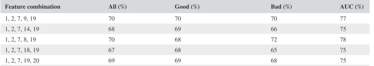
The final feature combinations selected from the LR are further tested on out-of sample data. The results are shown in Tables 7–9. The columns of the tables below show the percentage of overall correctly classified obligors, the percentage of correctly classified good obligors, the percentage of the correctly classified bad obligors and the AUC on the out-of-sample data for LR.

The final feature combinations selected from the SVR are further tested on out-of-sample data. The results are shown in Table 10–12. The columns of the tables are analogous to those of Tables 7–9.

The results based on one out-of-sample dataset indicate that in terms of AUC the logistic regression should out-perform the SVM on all datasets. For the German data the AUC of the LR ranges from 75% to 78%, whereas the AUC of the SVM ranges from 70% to 77%. For the East-European data the AUC of the LR ranges from 67% to 69%, whereas the AUC of the SVM ranges from 64% to 70%. For the Polish data the AUC of the LR ranges from 81% to 93%, whereas the AUC of the SVM ranges from 80% to 84%. However, the percentage of the overall correctly classified obligors is a better measure of classification

TABLE 1 Final feature combinations for LR, German retail data

Feature combination BIC AIC AUC (%)

1, 2, 7, 9, 19 250.22 270.01 77.94

1, 2, 7, 14, 19 245.43 265.22 77.71

1, 2, 7, 8, 19 249.26 269.05 77.70

1, 2, 7, 18, 19 250.28 270.07 77.49

1, 2, 7, 19, 20 249.26 269.05 77.48

Note: Area under the curve (AUC), Akaike information criterion (AIC) and Bayes information criterion (BIC) on test (validation) data. TABLE 2 Final feature combinations for LR, East-European corporate data

1, 8, 14, 25, 30, 32 1,019.43 1,053.20 77.92

1, 14, 25, 30, 32, 33 1,024.97 1,058.74 77.84

1, 13, 14, 25, 30, 32 1,024.67 1,058.45 77.80

8, 9, 14, 26, 29, 30 997.45 1,031.22 77.58

9, 11, 14, 25, 29, 30 958.74 992.51 77.55

Note: Area under the curve (AUC), Akaike information criterion (AIC) and Bayes information criterion (BIC) on test (validation) data. TABLE 3 Final feature combinations for LR, Polish corporate data

2, 21, 26, 34, 39 462.11 486.06 84.85

2, 21, 34, 39, 45 466.38 490.34 84.33

2, 11, 21, 34, 39 464.94 488.89 83.93

6, 32, 43, 55, 56 473.58 497.53 83.69

2, 11, 34, 39, 45 465.78 489.73 83.59

Note: Area under the curve (AUC), Akaike information criterion (AIC) and Bayes information criterion (BIC) on test (validation) data. TABLE 4 Final feature combinations for SVM, German retail data

Feature combination Distance Number of SV AUC (%)

1, 11, 13, 14, 15 0.119 153 79.45

1, 10, 13, 14, 15 0.077 152 79.34

1, 4, 10, 13, 14 0.062 148 79.13

1, 4, 13, 14, 19 0.055 152 78.98

1, 2, 6, 11, 17 0.072 151 78.90

(9)

TABLE 6 Final feature combinations for SVM, Polish corporate data

2, 26, 39 0.196 309 83.79

2, 11, 39 0.177 310 83.74

2, 39, 45 0.181 310 83.72

2, 21, 39 0.181 310 83.72

2, 26, 34, 39, 55 0.272 309 83.71

Note: Area under the curve (AUC), distance to the hyperplane and number of support vectors on test (validation) data. TABLE 5 Final feature combinations for SVM, East-European corporate data

9, 14, 25, 30 0.437 554 75.09

14, 25 0.159 588 74.95

1, 6, 30 0.155 568 74.82

9, 25, 30 0.061 588 74.26

1, 25, 30 0.066 568 74.10

Note: Area under the curve (AUC), distance to the hyperplane and number of support vectors on test (validation) data.

TABLE 7 Final feature combinations for LR, out-of-sample German retail data

Feature combination All (%) Good (%) Bad (%) AUC (%)

1, 2, 7, 9, 19 70 70 70 77

1, 2, 7, 14, 19 68 69 66 75

1, 2, 7, 8, 19 70 68 72 78

1, 2, 7, 18, 19 67 68 65 75

1, 2, 7, 19, 20 69 69 68 75

Note: Percentage of correctly classified (All), percentage of the correctly classified bad obligors (Bad), percentage of the correctly classified good obligors (Good), and area under the curve (AUC).

TABLE 8 Final feature combinations for LR, out of sample East-European corporate data

1, 8, 14, 25, 30, 32 62 60 63 69

1, 14, 25, 30, 32, 33 61 63 58 67

1, 13, 14, 25, 30, 32 60 62 58 67

8, 9, 14, 26, 29, 30 65 58 71 67

9, 11, 14, 25, 29, 30 62 55 70 69

TABLE 9 Final feature combinations for LR, out of sample Polish corporate data

2, 21, 26, 34, 39 87 85 89 93

2, 21, 34, 39, 45 88 87 88 93

2, 11, 21, 34, 39 87 86 88 92

6, 32, 43, 55, 56 71 80 61 81

2, 11, 34, 39, 45 81 83 79 89

(10)

accuracy, whereas the AUC is a rank-ordering measure. In terms of correctly classified obligors, the SVM out-performs the LR for the German and the East-European data, see column “All” in Tables 10–12. Only on the Polish data the LR shows superior performance.

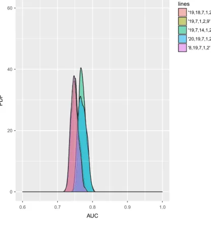
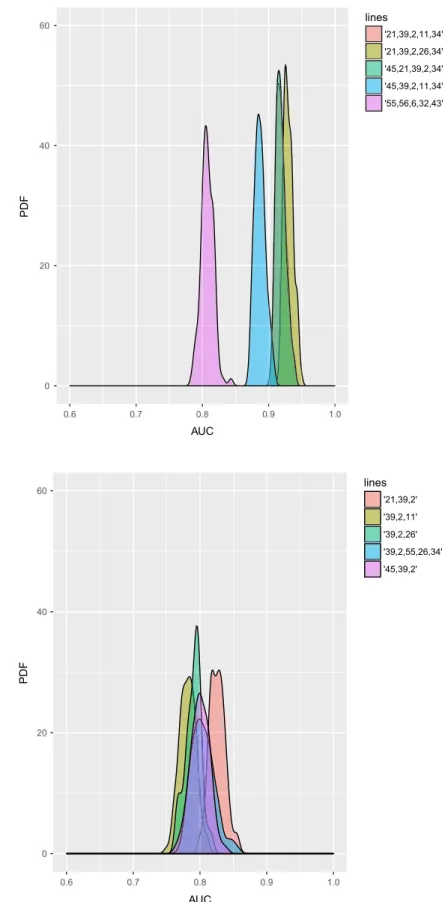
For that reason, the final feature combinations selected from the LR and the SVM models are further tested 100 times with different out-of-sample datasets (subsets of the main out-of-sample dataset). Figures 3–8 show the results. Clearly the SVM gives a higher AUC when tested on multiple out-of-sample datasets. The only exception is the Polish corporate data where the LR produces a higher AUC.

3.5 | Comparison of the variable selection method to an alternative variable selection method

Table 13 presents the output of the sequential variable selection method implemented in MATLAB. Hira and Gillies (2015) provide a comprehensive discussion on feature selection methods. The results show that the proposed variable selection method performs similarly to the challenger selection method on the of sample data. On the Polish data, the proposed method out-performs significantly the alternative variable selection method.

We further test the performance of the challenger sequential variable selection method 100 times with different out-of-sample datasets (subsets of the main out-of-sample dataset). In this case, we show that the performance of the

TABLE 10 Final feature combinations for SVM, out-of-sample German retail data

1, 11, 13, 14, 15 70 64 75 70

1, 10, 13, 14, 15 69 58 79 71

1, 4, 10, 13, 14 71 59 83 72

1, 4, 13, 14, 19 73 65 81 74

1, 2, 6, 11, 17 76 78 74 77

TABLE 11 Final feature combinations for SVM, East-European corporate out-of-sample data

9, 14, 25, 30 70 70 69 69

14, 25 64 52 76 64

1, 6, 30 70 65 74 70

9, 25, 30 66 68 64 66

9, 25, 30 70 72 67 70

TABLE 12 Final feature combinations for SVM, Polish corporate out-of-sample data

2, 26, 39 79 83 74 80

2, 11, 39 79 83 74 80

2, 39, 45 79 83 74 82

2, 21, 39 83 83 83 84

2, 26, 34, 39, 55 81 76 85 81

(11)

proposed selection method works well for the SVM when it is based on the distance to the hyperplane. The SVM distance to the hyperplane method outperforms the challenger method on all datasets as can be seen by comparing Figures 4, 6 and 8 with Figures 10, 12 and 14. In the case of LR, where we do not use the distance to the hyperplane and the number

FIGURE 3 Area under the curve (AUC) distribution on out-of-sample German retail data, LR

0 20 40 60 0.6 0.7 0.8 0.9 1.0 AUC PD F lines '19,18,7,1,2' '19,7,1,2,9' '19,7,14,1,2' '20,19,7,1,2' '8,19,7,1,2'

FIGURE 4 Area under the curve (AUC) distribution on out-of-sample German retail data, SVM

0 20 40 60 0.6 0.7 0.8 0.9 1.0 AUC PD F lines '11,17,2,6,1' '14,13,1,4,10' '14,13,1,4,19' '14,13,15,1,10' '14,13,15,1,11'

(12)

of support vectors (this is possible only for SVM), the proposed method has similar performance and LR outperforms the challenger only on the Polish data, as can be seen by comparing Figures 3, 5 and 7 with Figures 9, 11 and 13. However, this is due to the fact that in general LR is a more suitable method for that dataset as can be concluded when compared to the SVM.

FIGURE 5 Area under the curve (AUC) distribution on out-of-sample East-European corporate data, LR

0 20 40 60 0.6 0.7 0.8 0.9 1.0 AUC PD F lines '14,32,13,30,25,1' '14,32,30,25,1,8' '33,14,32,30,25,1' '9,25,30,14,29,11' '9,8,30,26,14,29'

FIGURE 6 Area under the curve (AUC) distribution on out-of-sample East-European corporate data, SVM

0 20 40 60 0.6 0.7 0.8 0.9 1.0 AUC PD F lines '14,25' '30,25,1' '6,30,1' '9,25,30' '9,25,30,14'

(13)

4 | MANAGERIAL INSIGHTS

The economic interpretation of the final results is important. For that reason we identify the most frequent default drivers in each dataset. Referring back to tables, Tables 7–13 and counting the occurrence of variables in both models (LR and SVM)

FIGURE 8 Area under the curve (AUC) distribution on out-of-sample Polish corporate data, SVM 0 20 40 60 0.6 0.7 0.8 0.9 1.0 AUC PD F lines '21,39,2' '39,2,11' '39,2,26' '39,2,55,26,34' '45,39,2' FIGURE 7 Area under the curve

(AUC) distribution on out-of-sample Polish corporate data, LR 0 20 40 60 0.6 0.7 0.8 0.9 1.0 AUC PD F lines '21,39,2,11,34' '21,39,2,26,34' '45,21,39,2,34' '45,39,2,11,34' '55,56,6,32,43'

(14)

we present in Table 14 the occurrence of each feature in each dataset. Then we compare the most frequent variables from the proposed variable selection method to the ones given by the challenger variable selection method. If possible, we identify the common features between the two methods considering only those variables from the proposed method that appear at least six times (in 50% of the cases, we have 10 final models for each dataset). For the Polish dataset there is no common frequent vari-ables between the two methods and therefore we further discuss the varivari-ables from the proposed method only.

Following the logic described above we have identified the following common variables:

1. For the German retail data the most common variables across the two selection methods are as follows: status of existing checking account, duration of the account in months and phone number availability.

2. For the East-European corporate data the most common variables across the two selection methods are as follows: earn-ings on operating income and total assets.

3. For the Polish corporate data, the most common variables are: total liabilities/total assets and profit on sales/sales. The results are shown in Table 15.

One explanation for the total assets to significantly affect the PD is that the change in total assets is related to business growth. If a business grows substantially in terms of assets, this means that large long-term investments were made in that business. All other factors being equal, the long-term investments will result in higher profit if the company keeps the same

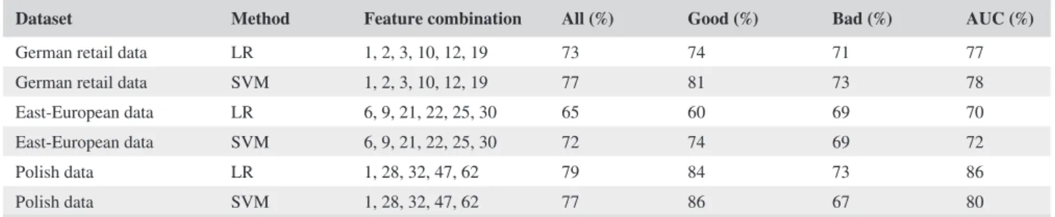
FIGURE 9 Area under the curve (AUC) distribution on out-of-sample German retail data, LR

0 20 40 60 0.6 0.7 0.8 0.9 1.0 AUC PD F lines '1,2,3,10,12,19'

TABLE 13 Final feature combinations; challenger feature selection method applied to the out-of-sample data

Dataset Method Feature combination All (%) Good (%) Bad (%) AUC (%)

German retail data LR 1, 2, 3, 10, 12, 19 73 74 71 77

German retail data SVM 1, 2, 3, 10, 12, 19 77 81 73 78

East-European data LR 6, 9, 21, 22, 25, 30 65 60 69 70

East-European data SVM 6, 9, 21, 22, 25, 30 72 74 69 72

Polish data LR 1, 28, 32, 47, 62 79 84 73 86

Polish data SVM 1, 28, 32, 47, 62 77 86 67 80

(15)

level of operational risk. In the retail, the final variables that appear most are the “status of existing checking account” and the “duration in months of the checking account.”

The above difference in the most frequent ratios across the models and the datasets shows that model selection is not only a function of the best performing model but also a function of the business goals and the business environment of the lending institution.

FIGURE 10 Area under the curve (AUC) distribution on out-of-sample German retail data, SVM

0 20 40 60 0.6 0.7 0.8 0.9 1.0 AUC PD F lines '1,2,3,10,12,19'

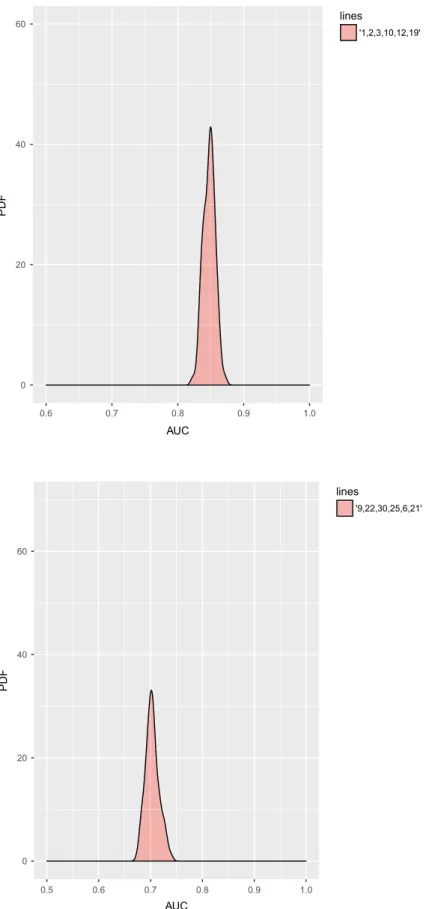
FIGURE 11 Area under the curve (AUC) distribution on out-of-sample East-European corporate data, LR

0 20 40 60 0.5 0.6 0.7 0.8 0.9 1.0 AUC PD F lines '9,22,30,25,6,21'

(16)

4.1 | Reference to the findings of other authors

Bellotti and Crook (2009) found that one of the most important factors for default estimation are “home owner status” and the “time with bank.” We also found that the time spent with the bank is a main indicator of default risk. However, Bellotti and

FIGURE 12 Area under the curve (AUC) distribution on out-of-sample East-European corporate data, SVM

0 20 40 60 0.6 0.7 0.8 0.9 1.0 AUC PD F lines '9,22,30,25,6,21'

FIGURE 13 Logistic regression, area under the curve (AUC) distribution on out-of-sample Polish corporate data

0 20 40 60 0.6 0.7 0.8 0.9 1.0 AUC PD F lines '28,62,1,32,47'

(17)

Crook (2009) found other significant indicators of default such as “total outstanding balance excluding mortgages on all active CAIS accounts” and “total number of credit searches in last 6 months.” In contrast, we did not identify similar variables to ap-pear frequently as default risk drivers. One reason is the fact the we kept the total number of variables down to five, whereas Bellotti and Crook (2009) used as many as eleven variables in their final model.

FIGURE 14 Support vector machines, area under the curve (AUC) distribution on out-of-sample Polish corporate data 0 20 40 60 0.6 0.7 0.8 0.9 1.0 AUC PD F lines '28,62,1,32,47'

TABLE 14 Selection of the most frequent variables on the test (validation) data across the three different data sets: German (G), East-European (E), Polish (P)

Id (G) Freq (G) Id (E) Freq (E) Id (P) Freq (P) Id (CV_G) Id (CV_E) Id (CV_P)

1 10 30 9 2 9 1 6 1 2 6 25 8 39 9 2 9 28 19 6 14 7 34 5 3 21 32 7 5 1 5 21 4 10 22 47 14 5 9 4 11 3 12 25 62 13 4 32 3 26 3 19 30 4 2 8 2 45 2 10 2 11 2 55 2 11 2 29 2 6 1 15 2 6 1 43 1 6 1 13 1 56 1 8 1 26 1 9 1 33 1 17 1 18 1 20 1

Notes: The last three columns are based on the challenger variable selection method applied to the datasets: German (CV_G), East-European (CV_E), Polish (CV_P); Id colums show the variable id in a given dataset, Freq columns show the number of times a variable appears in all the final variable combination (maximum can be 10, 5 models for LR and 5 models for SVM).

(18)

A study on wholesale data was done by (Chen et al., 2011). They found that the variable “account payable turnover” is a significant factor in measuring credit risk. The other seven variables proposed by Chen et al. (2011) were mainly based on the total assets and sales. Another interesting study is by (Hammer, Kogan, & Lejeune, 2012). They evaluated the creditworthi-ness of banks using statistical, as well as combinatorics-optimization logic-based methodologies. In their study, the Fitch risk ratings of banks were reversed-engineered using ordered logistic regression, SVM, and Logical Analysis of Data (LAD). They also indicated that total assets and liabilities play an important role in differentiating between good and bad obligors. This solidifies our findings and shows that although the individual factors can be slightly different, the major components of these factors are the same in both studies. This is also consistent with the findings of (Tian, Yu, & Guo, 2015). The business intuition is that the amount of the total assets relative to the liquid assets or other balance sheet items such as net profit provide a clear picture of how efficient the utilization of those assets by a particular obligor is. Minimizing the amount of total assets and maximizing the net profit is the objective of every private company. Another common default driver is the short-term (current) liabilities. This is consistent with the findings of Gök (2015). The business intuition is that current liabilities is a significant indicator of short-term debt. Companies with high levels of current liabilities in relation to other balance sheet items such as cash and sales are riskier and therefore they have a higher default probability. Finally we stress on that fact that although some differences exist between the Polish obligors and those of East-European obligors, most of the default drivers are the same, namely total assets, total liabilities and sales. This is consistent with the findings of Hosaka and Takata (2016).

5 | CONCLUSION

The findings of this research paper yield promising insights into the potential of SVM to estimate the probability of default (PD) of corporate and retail clients. Our work is consistent with the findings of Bellotti and Crook (2009) with respect to the usefulness of SVM for credit scoring.

Furthermore, we apply a wrapper approach for feature selection based on the distance of the support vectors from the sepa-rating hyperplane. We show that a combination of a wider hyperplane and fewer support vectors leads to a higher discrimination power for SVM.

From a financial point of view, the most frequently applied variables for PD estimation are total assets, total liabilities and sales in the corporate segment. In the retail segment the variables that appear most are current account status and duration of the current account.

Future work may include more experiments on estimating other Basel measures such as loss-given default (LGD) and ex-posure at default (EAD). Supervised nonlinear machine learning methods can be successfully applied for the estimation of PD, LGD and EAD in a way that accounts for their correlations. The collateral prices and their evolution, which are an important aspect of the capital calculations under the Basel guidelines, can also be modeled with nonlinear machine learning methods.

Overall, the SVM model proposed here shows promising results. Practically, this could save time and effort and will lead to making better-informed credit risk decisions.

ACKNOWLEDGEMENTS

The funding of the Systemic Risk Centre by the Economic and Social Research Council (ESRC) is gratefully acknowledged (grant number ES/K002309/1).

TABLE 15 Selected most frequent variables for each dataset, based on proposed and challenger variable selection methods

Dataset Variable ID Variable name

German 1 Status of existing checking account

German 2 Duration in months of the account

German 19 Telephone availability

East-European 25 Earnings on operating income

East-European 30 Total assets

Polish 2 Total liabilities/total assets

(19)

ORCID

Eduard Sariev https://orcid.org/0000-0003-2674-4166

Guido Germano https://orcid.org/0000-0003-4441-9842

REFERENCES

Abayomi, K., Gelman, A., & Levy, M. (2008). Diagnostics for multivariate imputations. Applied Statistics, 57 (3), 273–291. https://doi. org/10.1111/j.1467-9876.2007.00613.x

Balaji, S. A., & Baskaran, K. (2013). Design and development of an artificial neural networking (ANN) system using sigmoid activation function to predict annual rice production in Tamilnadu. International Journal of Computer Science, Engineering and Information Technology 3 (1), 13–31. https://doi.org/10.5121/ijcseit.2013.3102

BCBS. (2001). Basel committee on banking supervision. The internal ratings-based approach. Basel, Switzerland: Bank for International Settlements. Becker, N., Werft, W., Toedt, G., Lichter, P., & Benner, A. (2009). Penalized SVM: A R-package for feature selection SVM classification.

Bioinformatics, 25 (13), 1711–1712. https://doi.org/10.1093/bioinformatics/btp286

Bellotti, T., & Crook, J. (2009). Support vector machines for credit scoring and discovery of significant features. Expert Systems with Applications,

36 (2), 3302–3308. https://doi.org/10.1016/j.eswa.2008.01.005

Bellotti, T., Matousek, R., & Stewarti, C. (2011). A note comparing support vector machines and ordered choice models’ predictions of international banks’ ratings. Decision Support Systems. 51 (3), 682–687. https://doi.org/10.1016/j.dss.2011.03.008

Boser, B. E., Guyon, I. M., & Vapnik, V. N. (1992). A training algorithm for optimal margin classifiers. In: ACM special interest group for automata

and computability theory, Proceedings of the Fifth Annual Workshop on Computational Learning Theory. COLT ’92 (pp. 144–152). New York,

NY: Association for Computing Machinery. https://doi.org/10.1145/130385.130401

Box, G. E. P., & Cox, D. R. (1964). An analysis of transformations. Journal of the Royal Statistical Society, Series B, 26 (2), 211–252. http://www.jstor.org/stable/2984418

Broomhead, D., & Lowe, D. (1988). Multivariable functional interpolation and adaptive networks. Complex Systems, 35 (2), 321–355. https://www.bibsonomy.org/bibtex/24ef3a0adaabe7e13dcdeee339068f840/mcdiaz

Chang, C.-C., & Lin, C.-J. (2011). LIBSVM: A library for support vector machines. ACM Transactions on Intelligent Systems and Technology, 2 (3), 27:1–2727. https://www.csie.ntu.edu.tw/cjlin/papers/libsvm.pdf

Chen, Y.-W., & Lin, C.-J. (2006). Combining svms with various feature selection strategies. In: I. Guyon, M. Nikravesh, S. Gunn, & L. A. Zadeh (Eds.), Feature extraction: Foundations and applications (pp. 315–324). Berlin, Germany: Springer.

Chen, S., Härdle, W. K., & Moro, R. A. (2011). Modeling default risk with support vector machines. Quantitative Finance. 11 (1), 135–154. https:// doi.org/10.1080/14697680903410015

Cortes, C., & Vapnik, V. (1995). Support-vector networks. Machine Learning, 30 (3), 273–297. https://doi.org/10.1023/A:1022627411411

Cristianini, N., & Shawe-Taylor, J. (2000). An introduction to support vector machines and other kernel-based learning methods, Chapter 3. Cambridge, UK: Cambridge University Press.

Fan, R.-E., Chang, K.-W., Hsieh, C.-J., Wang, X.-R., & Lin, C.-J. (2012). LIBLINEAR: A library for large linear classification. Journal of Machine

Learning Research, 9, 1871–1874. https://doi.org/10.1145/1390681.1442794

Gavalas, D. (2015). How do banks perform under Basel III? Tracing lending rates and loan quantity. Journal of Economics and Business, 81 (September-October), 21–37. https://doi.org/10.1016/j.jeconbus.2015.0

Gök, M. (2015). An ensemble of k-nearest neighbours algorithm for detection of Parkinson's disease. International Journal of Systems Science, 46 (6), 1108–1112. https://doi.org/10.1080/00207721.2013.809613

Güneş, S., Polat, K., & Yosunkaya, Ç. (2010). Multi-class f-score feature selection approach to classification of obstructive sleep apnea syndrome.

Expert Systems with Applications, 37 (2), 998–1004. https://doi.org/10.1016/j.eswa.2009.05.075

Guyon, I., & Elisseeff, A. (2003). An introduction to variable and feature selection. Journal of Machine Learning Research, 3 (1), 1157–1182. http:// dl.acm.org/citation.cfm?id=944919.944968

Hammer, P. L., Kogan, A., & Lejeune, M. A. (2012). A logical analysis of banks financial strength ratings. Expert Systems with Applications 39 (9), 7808–7821. https://doi.org/10.2139/ssrn.975572

Han, J., & Moraga, C. (1995). The influence of the sigmoid function parameters on the speed of backpropagation learning. In: J. Mira & F. Sandoval (Eds.), From natural to artificial neural computation (pp. 195–201). Berlin, Germany: Springer, Proceedings of the International Workshop on Artificial Neural Networks, Malaga-Torremolinos, Spain, 7–9 June, 1995.

Harris, T. (2015). Credit scoring using the clustered support vector machine. Expert Systems with Applications 42 (2), 741–750. https://doi.org/10.1016/j.eswa.2014.08.029

Hens, A. B., & Tiwari, M. K. (2012). Computational time reduction for credit scoring: An integrated approach based on support vector machine and stratified sampling method. Expert Systems with Applications 39 (8), 6774–6781. https://doi.org/10.1016/j.eswa.2011.12.057

Hira, Z. M., & Gillies, D. F. (2015). A review of feature selection and feature extraction methods applied on microarray data. Advances in Bioinformatics

2015, 198363, 1–13. https://doi.org/10.1155/2015/198363

Hofmann, H. (1994). Statlog German credit data set. http://archive.ics.uci.edu/ml/datasets/Statlog+%28German+Credit+Data%29

Hosaka, T., & Takata, Y. (2016). Corporate bankruptcy forecast using RealAdaBoost. Information: An International Interdisciplinary Journal 19 (6B), 2285–2298. https://ci.nii.ac.jp/naid/40020905300/en/

(20)

Huang, S.-C., & Huang, M.-H. (2010). Using SVM with embedded recursive feature selections for credit rating forecasting. Journal of Statistics and

Management Systems, 13 (1), 165–177. https://doi.org/10.1080/09720510.2010.10701462

Huang, C.-L., Chen, M.-C., & Wang, C.-J. (2007). Credit scoring with a data mining approach based on support vector machines. Expert Systems with

Applications, 33 (4), 847–856. https://doi.org/10.1016/j.eswa.2006.07.007

Kuhn, M., & Johnson, K. (2013). Applied predictive modeling. New York, NY: Springer. https://doi.org/10.1007/978-1-4614-6849-3

Lessmann, S., Baesens, B., Seow, H.-V., & Thomas, L. C. (2015). Benchmarking state-of-the-art classification algorithms for credit scoring: An up-date of research. European Journal of Operational Research 247 (1), 124–136. https://doi.org/10.1016/j.ejor.2015.05.030

Li, S.-T., Shiue, W., & Huang, M.-H. (2006). The evaluation of consumer loans using support vector machines. Expert Systems with Applications, 30 (4), 772–782. https://doi.org/10.1016/j.eswa.2005.07.041

Meyer, D., Leisch, F., & Hornik, K. (2003). The support vector machine under test. Neurocomputing, 55 (1–2), 169–186. https://doi.org/10.1016/S0925-2312(03)00431-4

Mukherjee, S. (2003). Classifying microarray data using support vector machines. In: D. P. Berrar, W. Dubitzky, & M. Granzow, (Eds.), A practical

approach to microarray data analysis (pp. 166–185). New York, NY: Springer. https://doi.org/10.1007/0-306-47815-3_9

Onali, E., & Ginesti, G. (2014). Pre-adoption market reaction to IFRS 9: A cross-country event-study. Journal of Accounting and Public Policy, 33 (6), 628–637. https://doi.org/10.1016/j.jaccpubpol.2014.08.004

Platt, J. (2000). Probabilistic outputs for support vector machines and comparison to regularize likelihood methods. In: A. Smola, P. Bartlett, B. Schoelkopf, & D. Schuurmans (Eds.), Advances in large margin classifiers (pp. 61–74). Cambridge, MA: MIT Press. http://www.eecs.yorku.ca/course_archive/2005-06/F/6002B/Readings/lmc-book.pdf

Quanquan, G., Zhenhui, L., & Jiawei, H. (2011). Generalized fisher score for feature selection. In: Proceedings of the Twenty-Seventh Conference on

Uncertainty in Artificial Intelligence (pp. 266–273). Arlington, VA: AUAI Press. http://arxiv.org/abs/1205.2596

Rakotomamonjy, A. (2003). Variable selection using SVM-based criteria. Journal of Machine Learning Research 3, 1357–1370. http://dl.acm.org/citation.cfm?id=944919.944977

Rockafellar, R. T. (1993). Lagrange multipliers and optimality. SIAM Review 35 (2), 183–238. https://doi.org/10.1137/1035044

Tian, S., Yu, Y., & Guo, H. (2015). Variable selection and corporate bankruptcy forecasts. Journal of Banking & Finance 52 (Supplement C), 89–100. https://doi.org/10.1016/j.jbankfin.2014.12.003

Tomczak, S. (2016). Polish companies bankruptcy data set. https://archive.ics.uci.edu/ml/datasets/Polish+companies+bankruptcy+data/ Weston, J., Mukherjee, S., Chapelle, O., Pontil, M., Poggio, T., & Vapnik, V. (2000). Feature selection for SVMs. Advances in Neural Information

Processing Systems, 13, 668–674. http://papers.nips.cc/paper/1850-feature-selection-for-svms.pdf

How to cite this article: Sariev E, Germano G. An innovative feature selection method for support vector machines and its test on the estimation of the credit risk of default. Rev Financ Econ. 2018;00:1–24. https://doi.org/10.1002/rfe.1049

(21)

APPENDIX A

DESCRIPTIVE STATISTICS

TABLE A1 Summary statistics for all ratios, German retail data

Ratio number and name Median Mean

1 status of existing checking account 2 2.58

2 duration in months of the account 18 20.9

3 credit history 3 3.6

4 credit purpose 2 2.9

5 credit amount 2,320 3,271

6 savings account/bonds 1 2.1

7 present employment since 3 3.9

8 installment rate in percentage of disposable income 3 2.973

9 personal status and sex 3 2.7

10 other debtors/guarantors 1 1.2

11 present residence since 3 2.845

12 property indicator 2 2.4

13 age in years 33 35.55

14 other installment plans 3 2.7

15 housing indicator 2 1.9

16 number of existing credits at this bank 1 1.41

17 job status 3 2.9

18 number of people being liable to provide maintenance for 1 1.2

19 telephone availability 1 1.4

20 foreign worker indicator 1 1

(22)

TABLE A2 Summary statistics for all ratios, East-European data

Ratio name Mean Median Mean_i Median_i % Missing

1 return on assets (ROA) 0.13 0.08 0.13 0.08 0.00

2 ROA before financial expenses 0.18 0.13 0.18 0.12 0.00

3 return on operating income −0.07 0.08 −0.07 0.08 0.28

4 return on sales income −0.01 0.11 −0.01 0.11 0.44

5 return on investment 0.06 0.03 0.06 0.03 0.00

6 cash ratio 0.45 0.01 0.45 0.01 4.24

7 quick ratio 2.02 0.50 2.06 0.50 4.24

8 operating cash flow ratio 4.04 1.14 4.21 1.16 4.24

9 liquid assets over total assets 0.04 0.00 0.03 0.00 0.00

10 working capital over total assets 0.49 0.48 0.49 0.48 0.00

11 financial autonomy 6.67 0.64 14.25 20.34

12 total funding ratio 0.83 0.76 0.83 0.00

13 long term funding ratio 0.39 0.20 0.39 0.00

14 total financial liabilities over total assets 0.39 0.23 0.39 0.22 0.00

15 supply payables over total assets 0.16 0.09 0.16 0.09 0.00

16 financial liabilities over total liabilities 0.39 0.35 0.39 0.35 0.00

17 equity over total liabilities 2.01 0.29 2.04 0.29 1.88

18 short term funding ratio 0.62 0.68 0.62 0.68 1.88

19 total liabilities coverage 1.35 0.17 1.37 0.17 1.88

20 financial liabilities coverage 12.15 0.40 11.45 0.41 20.40

21 current financial liabilities coverage 7.30 0.87 84.54

22 interest coverage 47.44 4.17 99.86 4.43 16.17

23 earnings on assets 1.74 1.00 1.73 1.00 0.00

24 employees’ expense 0.13 0.06 0.13 0.06 0.44

25 earnings on operating income 1.10 0.95 1.10 0.94 0.44

26 payables turnover 243.32 39.27 263.44 39.30 0.89

27 inventory turnover 248.54 66.59 251.29 66.41 0.89

28 receivables turnover 96.08 20.27 97.17 20.27 0.44

29 total sales income 5,349 524 5348.68 524.00 0.00

30 total assets 3365 531 3365.22 531.00 0.00

31 relative annual change in total sales 2.37 0.12 4.62 0.14 33.00

32 relative annual change in total assets 1.13 0.16 1.34 0.15 32.94

33 relative annual change in profit from main

activities 4.33 −0.09 11.18 −0.08 34.28

34 absolute annual change in total liabilities 0.03 0.00 0.03 0.00 32.94

(23)

TABLE A3 Summary statistics for all ratios, Polish data

1 net profit/total assets −0.02 0.05 −0.02 0.05 0.00

2 total liabilities/total assets 0.47 0.45 0.47 0.45 0.00

3 working capital/total assets 0.19 0.22 0.19 0.22 0.00

4 current assets/short-term liabilities 4.89 1.65 4.89 1.66 0.00

5 (cash + short-term securities + receivables − short-term

liabilities)/(operating expenses − depreciation) × 365 19.41 0.49 19.41 0.57 0.00

6 retained earnings/total assets 0.02 0.00 0.02 0.00 0.00

7 EBIT/total assets −0.11 0.06 −0.11 0.06 0.00

8 book value of equity/total liabilities 5.74 1.15 5.74 1.16 0.00

9 sales/total assets 1.59 1.14 1.59 1.14 0.00

10 equity/total assets 0.55 0.52 0.55 0.52 0.00

11 (gross profit + extraordinary items + financial expenses)/

total assets −0.01 0.07 −0.01 0.07 0.00

12 gross profit/short-term liabilities 1.07 0.17 1.07 0.17 0.00

13 (gross profit + depreciation)/sales 0.35 0.07 0.35 0.07 0.00

14 gross profit + interest)/total assets −0.11 0.06 −0.11 0.06 0.00

15 (total liabilities × 365)/(gross profit + depreciation) 1,033.62 872.16 1,033.62 875.25 0.00

16 (gross profit + depreciation)/total liabilities 1.19 0.24 1.19 0.24 0.00

17 total assets/total liabilities 6.83 2.21 6.83 2.21 0.00

18 gross profit/total assets −0.10 0.06 −0.10 0.06 0.00

19 gross profit/sales −0.09 0.04 −0.09 0.04 0.00

20 (inventory × 365)/sales 56.67 38.62 56.67 38.62 0.00

21 sales(n)/sales(n − 1) 2.46 1.12 2.46 1.12 0.02

22 profit on operating activities/total assets −0.00 0.06 −0.00 0.06 0.00

23 net profit/sales −0.10 0.03 −0.10 0.03 0.00

24 gross profit(in 3 years)/total assets 0.14 0.16 0.14 0.16 0.02

25 (equity − share capital)/total assets 0.38 0.42 0.38 0.42 0.00

26 (net profit + depreciation)/total liabilities 1.09 0.21 1.09 0.21 0.00

27 profit on operating activities/financial expenses 463.64 0.98 463.64 1.15 0.07

28 working capital/fixed assets 10.23 0.53 10.23 0.55 0.02

29 logarithm of total assets 4.15 4.17 4.15 4.17 0.00

30 (total liabilities,cash)/sales 0.85 0.22 0.85 0.22 0.00

31 (gross profit + interest)/sales −0.07 0.04 −0.07 0.04 0.00

32 (current liabilities × 365)/cost of products sold 2111.59 81.13 2111.59 81.91 0.01

33 operating expenses/short-term liabilities 8.34 4.47 8.34 4.50 0.00

34 operating expenses/total liabilities 5.01 1.71 5.01 1.72 0.00

35 profit on sales/total assets −0.01 0.06 −0.01 0.06 0.00

36 total sales/total assets 2.05 1.56 2.05 1.56 0.00

37 (current assets,inventories)/long-term liabilities 114.03 3.66 67.02 5.00 0.43

38 constant capital/total assets 0.65 0.62 0.65 0.62 0.00

39 profit on sales/sales 0.02 0.04 0.02 0.04 0.00

40 (current assets,inventory/receivables)/short-term liabilities 2.21 0.18 2.21 0.18 0.00

41 total liabilities/((profit on operating

activities + depreciation) × (12/365)) 2.19 0.09 2.19 0.09 0.01

42 profit on operating activities/sales −0.02 0.04 −0.02 0.04 0.00

(24)

43 rotation receivables + inventory turnover in days 155.56 106.41 155.56 106.41 0.00

44 (receivables × 365)/sales 98.88 58.79 98.88 58.79 0.00

45 net profit/inventory 66.63 0.26 66.63 0.29 0.05

46 (current assets-inventory)/short-termliabilities 4.01 1.07 4.01 1.07 0.00

47 (inventory × 365)/cost of products sold 137.42 41.99 137.42 42.35 0.01

48 EBITDA(profit on operating activities − depreciation)/total

assets −0.09 0.02 −0.09 0.02 0.00

49 EBITDA(profit on operating activities − depreciation)/sales −0.07 0.01 −0.07 0.01 0.00

50 current assets/total liabilities 4.17 1.29 4.17 1.29 0.00

51 short-term liabilities/total assets 0.43 0.33 0.43 0.33 0.00

52 (short-term liabilities × 365)/cost of products sold) 0.73 0.22 0.73 0.22 0.01

53 equity/fixed assets 11.20 1.28 11.20 1.30 0.02

54 constant capital/fixed assets 12.11 1.43 12.11 1.45 0.02

55 working capital 10,817 1,803 10,817 1,803 0.00

56 (sales, cost of products sold)/sales 0.06 0.05 0.06 0.05 0.00

57 (current assets-inventory-short-term liabilities)/(sales-gross

profit-depreciation) −0.26 0.11 −0.26 0.11 0.00

58 total costs/total sales 0.96 0.95 0.96 0.95 0.00

59 long-term liabilities/equity 0.28 0.01 0.28 0.01 0.00

60 sales/inventory 911.03 9.04 911.03 9.45 0.05

61 sales/receivables 10.94 6.20 10.94 6.21 0.00

62 (short-term liabilities × 365)/sales 241.98 73.78 241.98 73.78 0.00

63 sales/short-term liabilities 9.13 4.93 9.13 4.94 0.00

64 sales/fixed assets 65.28 4.10 65.28 4.22 0.02

Notes: Mean, mean_i, median and median_i are the mean and median before and after imputation; % missing is the percentage of missing values.