Thirty Sixth International Conference on Information Systems, Fort Worth 2015 1
Using Big Data for Predicting Freshman
Retention
Completed Research Paper
Sudha Ram
University of Arizona, Management
Information Systems
Tucson, Arizona, United States
[email protected]
Yun Wang
University of Arizona, Management
Information Systems
Tucson, Arizona, United States
[email protected]
Faiz Currim
University of Arizona, Management
Information Systems
Tucson, Arizona, United States
[email protected]
Sabah Currim
University of Arizona, University
Analytics & Institutional Research
Tucson, Arizona, United States
[email protected]
Abstract
Traditional research in student retention is survey-based, relying on data collected from questionnaires, which is not optimal for proactive prediction and real-time decision (student intervention) support. Machine learning approaches have their own limitations. Therefore, in this research, we propose a big data approach to formulating a predictive model. We used commonly available (student demographic and academic) data in academic institutions augmented by derived implicit social networks from students’ university smart card transactions. Furthermore, we applied a sequence learning method to infer students’ campus integration from their purchasing behaviors. Since student retention data is highly imbalanced, we built a new ensemble classifier to predict students at-risk of dropping out. For model evaluation, we use a real-world dataset of smart card transactions from a large educational institution. The experimental results show that the addition of campus integration and social behavior features refined using the ensemble method significantly improve prediction accuracy and recall.
Keywords: Data mining, Machine learning, Predictive modeling, Social Network Analysis
Introduction
Student retention is an important outcome measurement to assess institutional performance. Improving retention rates is necessary for financial stability, graduation rates and institution reputation in higher education (Scott et al. 2004). It is a problem other stakeholders are deeply interested in, for example it’s estimated that state governments appropriated almost $6.2 billion between 2003 and 2008 to colleges and universities to help pay for the education of students who did not return to school for a second year (Schneider 2010). However, despite extensive efforts devoted to student retention, retaining students is still one of the most challenging problems faced by universities. The key to this problem is to identify students at risk of dropping out at an early stage, so that the institution can provide timely intervention to help those students proceed with their degrees. Traditional survey-based research has developed and validated a variety of theoretical models including Tinto’s student integration model (Tinto 1975), Astin’s theory of involvement (Astin 1999) and Beans’ student attrition model (Bean 1982). These theoretical models have identified multiple factors related to student retention and explained how they interact with each other. However, these methods are not easily applied in real-world scenarios such as real-time student intervention due to the drawbacks faced by survey-based data collection. The limitations of a survey approach include a time consuming and expensive data collection process (for a large-scale survey), low
participation rate and self-reporting biases(Cabrera et al. 1993). As an alternative, researchers have developed theoretical models using institutional student datasets (ISD) that contain demographics, educational background, economic status and academic progress. Empirical results indicate that both data sources are comparable, and ISD was found to be valuable in conducting institution-specific retention research under the constraint of limited resources (Caison 2007). To overcome this constraint, data mining techniques are getting more attention from student retention researchers because of their capacity for robust learning from large volumes of data and the ability to recognize hidden relationships among variables. This quantitative approach provides a much-needed complement for accurate and timely prediction of student attrition (Delen 2011).
Big data analytic methods have shown robust predictive power for multiple applications, yet, current research in student retention has not fully investigated their potential. Of particular interest to us is augmenting standard ISDs with resources that can infer student integration into campus life. From a feature exploration perspective, the traditional ISDs used in isolation are not sufficient to capture the dynamics of student behaviors on campus which leads to the loss of information about students’ social and campus integration (shown to be useful in predicting student retention). From a model-refinement perspective, the fact that drop-out students are the focus of prediction but have a much smaller sample size than retained students provides the opportunity of utilizing imbalanced classification techniques to improve the model sensitivity on the minority class. One recent study addressed this problem by using the synthetic minority over-sampling (SMOTE) method (Thammasiri et al. 2014). However, instead of using sampling methods alone, researchers have found that the integration of sampling methods with ensemble learning techniques can obtain better predictive performances (He and Garcia 2009).
In this research, we first extend the traditional ISD by including students’ behavioral patterns from their university smart card transactions. More specifically, we include two new forms of insight from transactional data: 1) implicit social networks derived from transactions based on their location and timestamp information; 2) sequences of locations visited by each student on a daily basis. From the implicit social network, we define novel network attributes to infer students’ level of social integration. Using our previously developed sequence learning algorithm (Wang and Ram 2015) on the sequential data, we are able to obtain students’ level of regularity in campus activities which helps measure their level of integration (i.e., based on regular use of campus facilities). To our knowledge, this is the first time implicit network interactions are being extracted from smart card usage to infer students' social and campus integration. Our experimental results show that the extended features (i.e., ISD + social patterns inferred from smart card transactions) make positive improvements to predictions based on using ISD alone. Based on this extended dataset, we developed and compared prediction models using two different data balancing techniques, SMOTE and SplitBal (Sun et al. 2015)with a stacking ensemble method. Our research demonstrates how Information Systems design science research using big data and predictive analytics can be beneficial in solving long-term and challenging problems in fields such as student retention.
The remainder of this paper is organized as follows: the Related Work section introduces previous work on student retention and data-balancing. The Methodology section describes the student dataset, our methods for feature extension, the prediction models and data balancing techniques applied in this research. The section Experimental Evaluation discusses the experimental setup and presents comparison results. The last section concludes the paper with future directions.
Related Work
Based on their basic underlying methodology, previous work on student retention can be categorized into behavioral vs. data-driven research. Research in both categories has identified significant factors that influence student retention but each category has certain limitations from a practical perspective.
Behavioral Approaches
Early efforts in student retention were mainly focused on building theoretical models. Fundamental theories that were developed are: Tinto’s student integration model (Tinto 1975), Astin’s theory of involvement (Astin 1999) and Bean’s student attrition model (Bean 1982). Tinto’s model was first built from the perspective of social integration which suggests that retained students are more socially integrated into the university. In this model, Tinto further distinguished social integration with academic integration where
Thirty Sixth International Conference on Information Systems, Fort Worth 2015 3 the social integration includes many aspects of students’ daily lives such as friendships, family support and feeling of satisfaction, and the academic integration contains the academic rules, norms and expectations. Later, Bean’s work provided an alternative explanation to student attrition where student’s decisions of departure are prompted by psychological beliefs which are further affected by students’ experience with different aspects of the institution such as institutional quality, faculty and friends. Similarly, Astin’s theory claims that students are most impacted by three types of involvement: with faculty, with academics and with peer groups. The greater the amounts of effort students invest in these involvements, the more likely they will persist. Although the three theories have different conceptual frameworks, the consensus is that student’s social integration and peer-relationship is an important indicator.
As a result of the above theoretical foundations, researchers have conducted other studies to identify additional variables that can predict student retention. Institutional and goal commitment are found to be significant for student retention (Cabrera et al. 1993; Sparkman et al. 2012). Another common agreement is that a student’s past academic progress like high school GPA and standardized test scores are significant in most settings (Reason 2009). Financial factors such as loans, grants and scholarships are reported as useful indicators in several studies (Cabrera et al. 1993; Herzog 2005; Reason 2009). Other than these variables, a sense of belonging (Hoffman et al. 2002) and parents’ education levels (Cabrera et al. 1993; Caison 2007) are notable factors that are proven to be useful. Since most of these studies rely on surveys to collect data to measure the factors mentioned above, it is not easy for institution administrations to apply these findings in practice (i.e., regularly survey students to identify at-risk sub-populations), particularly because those most at-risk of dropping out may have a lower feeling of institutional integration which may contribute to a lower response rate. Moreover, surveying is not cost-effective because the number of at-risk students is small compared to the number that retain. Therefore, we need to look for more readily available alternative data sources that can achieve similar goals.
Data-driven Approaches
The recent popularity of using a data-driven approach to student retention is facilitated by two facts. First, the amount of data stored in university data warehouses has increased rapidly. Student attributes like past academic performance, financial status and many other factors are readily available for use (Yadav and Pal 2012). From a big data perspective, we are able to complement ISDs with multiple secondary sources. Secondly, machine-based data analytics techniques are capable of discovering previously unknown relationships from large volumes of data. Also, this type of analytic technique is robust and adaptable to institution-specific settings (Caison 2007).
Most data-driven studies have trained their models on ISDs. Common variables used from ISDs are: demographics, high school GPA, standardized test scores and financial indicators, most of which are significant variables identified by behavioral studies. However, not all of the important theoretical variables have been captured in data-driven studies. For instance, it is uncommon to use traditional ISD to infer student’s social integration and their peer relationships. Researchers have suggested using a hybrid approach comprising survey and ISD-mining techniques to address this issue (Sarker et al. 2014; Thammasiri et al. 2014). Instead of waiting for survey results that make prediction and intervention for at-risk first-semester freshmen difficult, we argue that it is possible to analyze existing institutional resources to obtain comparable information.
This brings us to another issue that impacts the quality of training features. There is a trade-off between how early a prediction can be made for freshmen and the quality (accuracy and recall) of the prediction. The ideal situation is to identify at-risk students as early as possible, so that there is enough time to intervene on these students to retain them. Considering the fact that over fifty-percent of the student attrition can be attributed to drop-outs during the first year of study (Delen 2011), a prediction model will be more valuable if it can identify drop-out students as early as possible. As a result, studies (Delen 2011; Thammasiri et al. 2014) that used first semester GPA and reported it as the most influential variable in predicting first-year retention, do not offer the university administration the ability to identify and intervene on those students who did not return for the second semester. For such cases, it is critical to model and predict students who may need help before the end of first semester.
A goal of many data-driven studies is to find a classification algorithm that best predicts student retention. Researchers have tested and compared many families of classifiers including Naïve Bayes, Decision Trees, Neural Networks and Support Vector Machines (Delen 2011; Nandeshwar et al. 2011; Sarker et al. 2014;
Thammasiri et al. 2014). The main limitation of these classifiers is that they do not work effectively when the distribution of the dependent variable is imbalanced. A student retention dataset is naturally imbalanced, as in a typical university more students persist than drop out (e.g., about 80-85% of the population continues into the sophomore year). By default, classification algorithms assume approximately even-sized classes and tend to ignore the problem of minority classes (Sun et al. 2015). Past research has attempted to solve this problem using over-sampling (Lauría et al. 2012) and the SMOTE sampling technique (Thammasiri et al. 2014). Both techniques try to generate artificial samples for the minority class, and SMOTE is designed to overcome the over fitting issue of traditional oversampling. However, SMOTE has its own drawbacks including over-generalization and high variance (He and Garcia 2009).
In this work, we focus on the first-semester retention problem among freshmen, which has been insufficiently studied and is a target population identified as most likely in need of interventions (Herzog 2005). It is a difficult problem because university-level academic performance information is not yet available until after the first semester. In order to complement traditional ISD input features, we use university smart card transactions from which we extract and measure a variety of social network characteristics. Our previous research on students’ mobility behavior (Wang and Ram 2015) has shown that the implicit network derived from smart card transactions is a reliable indicator of their social relationship. We modified our sequence learning algorithm to evaluate the regularity with which students used campus activities. By using these two new features, we aim to infer the missed social and institutional integration information in current ISD-based studies. Regarding the problem of imbalanced data classes, we compare existing approaches with a state-of-the-art balancing technique (Sun et al. 2015) that also considers ensemble learning to boost performance.
Methodology
In this study, we consider the student retention prediction as a two-class prediction problem. As a supervised learning problem, the performance of a classifier relies on how effectively it can learn from the training set. One aspect that affects learning quality is the predictive power of the features. Another aspect is the amount of representative data. Imbalance due to rare instances will make the learning difficult. Therefore, we developed our model to address the issues of feature extraction and imbalanced learning. In this section, we introduce the variables obtained from an ISD. Then by comparing these with previous research findings, we identify the necessary features and design a new approach to extract features from smart card transactions, a data source that has not been considered before. Thereafter, we introduce our solution for imbalanced-class learning.
ISD Data
According to previous studies, freshmen are more prone to drop out, and identification of at-risk freshmen provides value for retention management (Herzog 2005; Thammasiri et al. 2014). In this study, we collected an anonymized ISD dataset for about 7000 freshmen corresponding to the academic year 2012 - 2013, from a large public university. Based on previous literature, we consider 21 variables that relate to different aspects of student demographics, sense of belonging, scholastic context, financial status, prior academic details and family background. We focused on full-time freshmen and cleaned the data by removing anomalies and samples with missing values. For example, we removed international students for whom SAT scores or high school GPAs were not available. The majority of the data points represented white domestic students under the age of 20, so we aggregated values for ethnicity, age ranges and citizenship into two categories each (represented by binary variables). Details of ISD variables are in Table 1.
After data cleaning, we were left with about 6500 students, of which 479 (7.37%) drop-out after Fall and 843 (12.98%) drop-out at the end of Spring. We distinguish the two drop-out groups, because some variables (e.g., ‘Fall GPA’, ‘Spring student loan’) are not available until the beginning the second semester. It is worth noting that first term GPA is found to be the most important predictor for first-year dropout rates (Delen 2011; Thammasiri et al. 2014); thus, predicting first semester drop-out students is harder than predicting those who drop-out after the second semester because of the lack of key information.
Thirty Sixth International Conference on Information Systems, Fort Worth 2015 5
Table 1. ISD Variables
Perspective Variables Definition Type
Demographics Ethnic White = 1, Others = 0 Binary
Age range ‘Less or equal to 20’ = 1,
Others = 0 Binary
Gender Female = 1, Male = 0 Binary
Citizenship US = 1, Others = 0 Binary
In-state student In-state = 1, Others = 0 Binary
Sense of belonging On-campus employment Employed = 1, Unemployed
= 0 Binary
Living community Joined = 1, Not joined = 0 Binary
Accommodation On-campus = 1, Others = 0 Binary
Scholastic context Major 0-25: Top 25 based on
population, 26:Others Nominal
College 0-16: 17 Colleges Nominal
Honors student Yes= 1, No = 0 Binary
Course units enrolled >= 12 to be full-time Number
Financial status Fall student loan Yes= 1, No = 0 Binary
Fall tuition waive Yes= 1, No = 0 Binary
Prior academic
details High school GPASAT comprehensive Z-score normalizedZ-score normalized NumberNumber
Advanced program Enrolled = 1, Not enrolled =
0 Binary
Family background First generation student Yes = 1, No = 0 Binary
Pattern Extraction from Implicit Networks
Nearly all the fundamental theories have emphasized the importance of social integration in student retention (Astin 1999; Bean 1982; Tinto 1975). However, students’ social relationships are usually not accessible through a standard ISD and usually inferred using questionnaires and surveys. To address this issue, we propose an approach to infer student peer relationships by exploring their smart card transactions. For our study, we use the university smart card transaction dataset containing approximately 1.8million transactions made by freshmen. Each transaction provides information that includes location on campus (can be used to infer geographical information) and type of service (e.g., restaurant, printer services, parking, vending machine, etc.). For privacy, some of the information is masked (e.g., the ID is anonymized and spatiotemporal details are aggregated to a higher granularity). Formally we represent a smart card transaction as follows. Let 𝑈 = {𝑢1, 𝑢2, … , 𝑢𝑛} be the set of sampled students, Σbe the set of
unique locations, then the smart card transactions can be denoted as a set of tuples 𝑇 = {< 𝑢𝑖, 𝑣𝑗, 𝑡𝑘>
|where 𝑢𝑖∈ 𝑈, 𝑣𝑗 ∈ Σ and 𝑡𝑘is a minute-level timestamp}. To infer students’ social integration, we generate implicit networks from smart card transactions. Then we define the metrics on our networks to reflect students’ dynamically changing relationships.
Implicit Network of Students
Although smart card data does not contain explicit information about student relationships, an observation is that some pairs of students make transactions at the same place and time with a considerable frequency. If we reason that students making purchase together may have a latent relationship, then based on this assumption, we can define directed implicit networks in which every node is a student and the edges connecting two nodes represent their latent relationship. A directed weighted edge indicates how important the successor is to the predecessor in terms of socialization. This latent relationship is asymmetric. For instance, suppose student B has only one friend, student A, on campus (A is the only student connected with B in a network), but A can have many friends (i.e., edges to other students in the network).
Considering student social relationships may change over time, we generate networks on a biweekly basis. After removing weekends and holidays (when few transactions happen on campus), we generated 8
networks for each semester. Let the networks be denoted as 𝐷𝑝(𝑉𝑝, 𝐸𝑝) for p = 1 to 16 where 𝑉𝑝is the set of nodes (𝑉𝑝⊂ 𝑈) and 𝐸𝑝 is the set of edges in 𝐷𝑝. We then generate network 𝐷𝑝 by adding nodes to 𝑉𝑝 and adding edges to 𝐸𝑝. During the two-week time window of 𝐷𝑝, if two students 𝑢𝑖, 𝑢𝑗∈ 𝑈 made transactions at the same location within a time interval 𝜏 at least 𝜋 times, we connect them together and add both nodes 𝑢𝑖, 𝑢𝑗to 𝑉𝑝 and directed edges 𝑒𝑖→𝑗 and 𝑒𝑗→𝑖 to 𝐸𝑝. Then the weight of directed edge 𝑒𝑖→𝑗 representing the strength of latent relationship is defined as:
𝑤𝑖→𝑗=
𝐶𝑖𝑗𝑝 ∑ℎ∈𝑁𝑖 𝐶𝑖ℎ𝑝
𝑝
ℎ
where 𝑁𝑖𝑝is the set of neighbors of 𝑢𝑖in 𝐷𝑝 and 𝐶𝑖𝑗
𝑝 is the number of times
𝑢𝑖, 𝑢𝑗 made transactions together during the two-week time window of 𝐷𝑝.
The complexity of each implicit network is controlled by 𝜏 and 𝜋. Decreasing the value of 𝜏 or increasing the value of 𝜋 can reduce the bias caused by randomness but the tradeoff is that the network will become sparse. A sparse network might not be able to accurately infer student peer relationships. In this study we set 𝜏 as 1 minute which was the most restrictive value possible with the transaction granularity available to us. Then we examined the decreasing rate of the number of edges by increasing the value of 𝜋. All the networks showed a stable decreasing rate when 𝜋 is larger than 3. Taking one of the networks as an example, Figure 1 (a) indicates an ‘elbow’ point at 𝜋=3. On average, we observe a 96% drop rate when 𝜋 is increased from 1 to 2 and a 43% drop rate when 𝜋 is increased from 3 to 4. This suggests that a number of random relationships are removed when 𝜋 is larger than 1. Hence, we set 𝜋 to 3 to preserve a balance between removing bias and network complexity. Under this parameter configuration, the 16 networks we generated have 2,200 connected nodes and 5,200 edges on average. The largest network is from the middle of the first semester and contains 2,400 nodes and 5,800 edges. The last (end of semester) network is the smallest one with 1,700 nodes and 3,100 edges. In order to further validate our networks, we compared the common location ratio (CLR) among students in the network with CLR among students not in the network, where the CLR of two students is defined as: 𝐶𝐿𝑅 =|𝐿𝑖∩𝐿𝑗|
|𝐿𝑖∪𝐿𝑗| where 𝐿𝑖 and 𝐿𝑗 are the sets of locations that have been visited by 𝑢𝑖 and 𝑢𝑗 respectively. Figure 1 (b) shows that students in the network have more common locations than those not in the network.
Figure 1. (a) Selecting π; (b) Common Location Ratio Network Features
The purpose of generating networks from smart card transactions is to infer student social integration. We are interested in metrics that can approximate questions like “How many friends does a student have?”,
Thirty Sixth International Conference on Information Systems, Fort Worth 2015 7
“What is the social activity level of a student?” or “Does a student have consistent interactions on campus?” To help us obtain these kinds of information from the networks, we defined 8 network features which can be grouped into 3 categories: A) node appearance metrics; B) degree metrics; C) edge metrics. All these features are measured for each individual on all the networks generated during a period of interest which can be an academic year, an entire semester or consecutive months during a semester. Assume the period of interest contains a set of networks {𝐷𝑗(𝑉𝑗, 𝐸𝑗)| where 𝑚 ≤ 𝑗 ≤ 𝑛}, we provide formal definitions of network features in the remainder of this section.
A. Node appearance metrics
Recall that the networks are generated every two weeks, and the more often a student (node) appears in these networks, the higher his or her inferred social activity level. We define two metrics, i.e., the number of appearance periods (NAP) and the longest consecutive number of appearance periods (LCAP). For every student 𝑢𝑖∈ 𝑈, we compute NAP and LCAP as:
𝑁𝐴𝑃( 𝑢𝑖) = ∑𝑛𝑗=𝑚𝐴𝑖𝑗
𝐿𝐶𝐴𝑃( 𝑢𝑖) = (𝑞 − 𝑝 + 1) conditioned on 𝐴𝑟𝑔𝑚𝑎𝑥𝑝,𝑞(∏𝑗=𝑝𝑞 𝐴𝑖𝑗∑𝑞𝑗=𝑝𝐴𝑖𝑗)
where 𝐴𝑖𝑗= 1 if 𝑢𝑖∈ 𝑉𝑗, otherwise 𝐴𝑖𝑗= 0 and 𝑚 ≤ 𝑝 ≤ 𝑞 ≤ 𝑛. We use NAP to capture the level of social activity on average and LCAP to measure the consistency of social activity.
B. Degree metrics
The degrees of a node in the network indicate the size of a student’s social circle which can be stable, growing or shrinking during the interest period. These different trends are useful for inferring students’ social integration. Given a node and its degrees in each of the period networks, we measure three degree related features: (1) average degree (AD); (2) standard deviation of degree (SDD); (3) the ratio of average degree (RAD) between the second half of networks (corresponding to first half of the semester) and the first half of networks. Similarly, for each student 𝑢𝑖∈ 𝑈, we compute AD, SDD and RAD as:
𝐴𝐷( 𝑢𝑖) = 1 𝑛−𝑚+1∑ 𝑑𝑖𝑗 𝑛 𝑗=𝑚 𝑆𝐷𝐷( 𝑢𝑖) = √ 1 𝑛−𝑚+1∑ (𝑑𝑖𝑗− 𝐴𝐷( 𝑢𝑖)) 2 𝑛 𝑗=𝑚 𝑅𝐴𝐷( 𝑢𝑖) = (⌊𝑛−𝑚+12 ⌋−𝑚+1) ∑𝑛 𝑑𝑖𝑗 𝑗=⌊𝑛−𝑚+12 ⌋+1 (𝑛−⌊𝑛−𝑚+1 2 ⌋+1) ∑ 𝑑𝑖𝑗 ⌊𝑛−𝑚+12 ⌋ 𝑗=𝑚
where 𝑑𝑖𝑗 is the out-degree of 𝑢𝑖 in 𝐷𝑗. According to the definition, AD measures the size of a student’s social circle, SDD measures how stable it is. We believe drop-out students may have a shrinking social circle, and we use RAD to capture this pattern.
C. Edge metrics
As discussed above, edges in our implicit network reflect a latent relationship between students. The weight, 𝑤𝑖→𝑗 of an outgoing edge indicates how important the successor is to the predecessor. The maximum weight of 1 indicates that the predecessor’s only transactions are with the successor (or alone). On the contrary, a relatively low outgoing weight suggests that although there is a latent relationship between predecessor and successor, the predecessor makes a significant number of transactions with students other than the successor. We are interested in measuring if a student in the network has strongly connected peers. Formally, let the edge 𝑒𝑖→𝑗connecting 𝑢𝑖 and 𝑢𝑗 be a strong connection if it meets two criteria: (1) 𝑤𝑖→𝑗is larger than 0.3; (2) 𝑢𝑖 and 𝑢𝑗 made at least 5 transactions together during the biweekly period. The parameters to define a strong connection are heuristically determined, where 0.3 is the average weight in networks and ‘at least 5 transactions’ requires a pair of students to purchase together every two weekdays on average during the biweekly time window.
Based on this definition of strong connection, we further designed three edge related metrics: (1) proportion of strong out-going edges (PSOE); (2) Among strong out-going edges, the probability that the paired in-coming edge is also strong (PSIE); (3) The probability of an edge in the first network 𝐷𝑛 being a ‘loyal’ edge (PLE), where we define an edge as ‘loyal’ if the two nodes are continuously connected in all networks from 𝐷𝑛 to 𝐷𝑚. We can compute the three metrics using the following equations:
𝑃𝑆𝑂𝐸( 𝑢𝑖) = 1 𝑛−𝑚+1∑ ∑𝑘∈𝑁𝑖𝑆𝑖𝑘𝑗 𝑗 𝑘 |𝑁𝑖 𝑗| 𝑛 𝑗=𝑚 𝑃𝑆𝐼𝐸( 𝑢𝑖) = 1 𝑛−𝑚+1∑ ∑𝑘∈𝑁𝑖𝑃𝑖𝑘𝑗 𝑗 𝑘 ∑𝑘∈𝑁𝑖𝑆𝑖𝑘𝑗 𝑗 𝑘 𝑛 𝑗=𝑚 𝑃𝐿𝐸( 𝑢𝑖) = ∑𝑘∈𝑁𝑖 𝐿𝑚𝑖𝑘 𝑚 𝑘 |𝑁𝑖 𝑚| where 𝑆𝑖𝑘𝑗 = 1 if 𝑤𝑖→𝑘> 0.3 and 𝐶𝑖𝑘 𝑗 > 5, otherwise 𝑆𝑖𝑘𝑗 = 0; 𝑃𝑖𝑘𝑗 = 1 if 𝑤𝑖→𝑘> 0.3, 𝑤𝑘→𝑖> 0.3and 𝐶𝑖𝑘 𝑗 > 5, otherwise 𝑃𝑖𝑘𝑗 = 0; 𝐿𝑚𝑖𝑘= 1 if 𝑒𝑖→𝑘∈ 𝐸𝑥 for ∀𝑥; 𝑚 < 𝑥 ≤ n, otherwise 𝐿𝑚𝑖𝑘= 0. Recall that 𝑁𝑖
𝑗is the set of neighbors of 𝑢𝑖in 𝐷𝑗, 𝐶𝑖𝑘
𝑗 is the number of times
𝑢𝑖, 𝑢𝑘 made transactions together during the time window of 𝐷𝑗, 𝑤𝑖→𝑘 is the weight of edge 𝑒𝑖→𝑘, and 𝐸𝑥 is the edge set of 𝐷𝑥.
To evaluate how these implicit networks can help us identify at-risk students, we used the 8 networks from the Fall semester and calculated the network metrics for continuing students and drop-out students separately. In addition, we segmented students in each class based on their Fall GPA. Average statistics of network metrics for each sub-group are shown in Table 2. In general, continuing students have higher social activity levels than drop-out students. In particular, drop-out students with GPA above 3.0 are least sociable compared with other groups of students, considering they have lowest NAP, LCAP, AD and PLE. Our network metrics provide a new perspective for the universities to identify these academically qualified students whom they mostly wanted to retain. To reinforce our findings from network metrics, we also calculate the proportion of social smart card transactions among all transactions. The result indicates that students in the continuing group have an average of 16.17% social transactions. The same statistic of students in the drop-out group is only 0.7% (two sample t-test, p < 0.001). A social transaction is a transaction made by a student with a neighbor in the implicit networks. Recall that a student is connected to another student if he made at least 𝜋 transactions within a time window 𝜏 during a two-week period.
Table 2. Average Network Metrics
GPA below 2.0 GPA between 2.0 to 3.0 GPA above 3.0
+ - t-test + - t-test + - t-test
NAP 0.49 2.33 9.30*** 0.60 2.33 6.58*** 0.23 1.87 6.52*** LCAP 0.58 2.69 9.90*** 0.67 2.71 7.26*** 0.28 2.174 7.04*** AD 0.25 1.06 4.96*** 0.26 0.84 3.66*** 0.08 0.58 3.97*** SDD 0.23 0.90 4.42*** 0.24 0.67 3.23** 0.09 0.43 3.36*** RAD 0.08 0.41 5.58*** 0.13 0.42 4.03*** 0.03 0.34 4.86*** PSOE 0.01 0.07 5.86*** 0.01 0.08 5.00*** 0.02 0.07 3.92*** PSIE 0.03 0.14 5.53*** 0.02 0.15 4.83*** 0.03 0.14 3.80*** PLE 0.01 0.02 2.00* 0 0.04 2.37* 0 0.09 2.35* * significant at p < 0.05; ** significant at p < 0.005; *** significant at p < 0.001 ‘+’ = drop-out students group; ‘-’ = continuing student group
Thirty Sixth International Conference on Information Systems, Fort Worth 2015 9
Pattern Extraction from Spatial (Location) Sequences
As discussed earlier, smart card transactions are represented as a set of tuples T = {< 𝑢𝑖, 𝑣𝑗, 𝑡𝑘>
|where 𝑢𝑖∈ 𝑈, 𝑣𝑗 ∈ Σ and 𝑡𝑘is a timestamp} in which the location set Σ represents various types of services provided on campus. Each smart card transaction is then an instance of a student interacting with the campus environment. Given the research finding that better integration into campus life leads to higher chance of retention, location information in the transaction data provides a unique source to extract patterns for retention prediction. For example, we can use the volume and frequency of smart card usage to infer students’ level of campus integration (in terms of use of campus facilities). Furthermore, if we extract locations from these tuples and order them in a sequence based on their timestamp, we can obtain a trajectory of students’ activities on campus. Previous research (Wang and Ram 2015) has found that these location sequences exhibit spatial and temporal patterns that can be used to predict students’ future locations. Such patterns are formed by different aspects of campus life such as class schedules, community activities and living conditions.
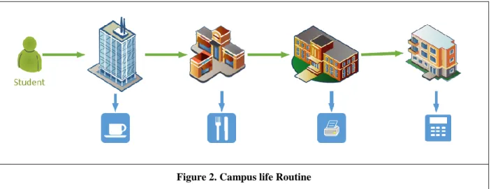
As illustrated in Figure 2, consider a student who has a morning class on a specific weekday, so she buys a cup of coffee near the classroom location before going to the lecture. At noon, she goes to the food court for lunch. In the evening, she attends a study group in the library and uses the printer there. Thereafter she returns to the dorm and buys a snack from the vending machine. If this is a regular routine of this student, we can observe a recurrence sequence of locations as ‘coffee shop, restaurant, library printer, dorm vending machine’ in her historical records. A repeated pattern detected from location sequences can reveal an individual’s daily routine on campus.
Returning to our original question, the purpose of investigating location sequences is to infer students’ campus integration. In this study, we assume that students who have a higher volume of smart card transactions and more predictable purchasing behaviors are better integrated into campus life. Next, we show the necessity of location clustering to make the sequential learning more reliable. Thereafter we introduce our metrics for measuring students’ level of regularity in their purchasing behavior.
Figure 2. Campus life Routine
Location Clustering
As per our assumption, frequent sequential patterns can reveal campus life routines. However, the same routine may be exhibited as different patterns. Taking Figure 2 as an example, if the student chooses one restaurant from a set of three every time she goes to the food court, we may observe three frequent patterns that are the same except for the restaurant’s name. Similarly, based on the example, using either the vending machine or a printer may reveal the fact that the student is in a dorm. It is useful to combine these patterns into one, because we can add up their frequencies to get a single pattern with higher frequency which can strengthen our assumption that it is formed by a regular routine.
Our solution for combing these patterns is to cluster locations. Locations can be grouped together based on their spatial proximity and social similarities. We define locations as socially similar if they are frequently visited by the same students. To be more specific, we created an undirected graph where the nodes are unique locations. Formally, let 𝐺(Σ, 𝐸) be the location graph where location set Σ becomes the set of vertices. For every location 𝑙𝑖∈ Σ, we represent it as a vector χ𝑖= [𝑐1, 𝑐2, … 𝑐|𝑈|] where 𝑐𝑘 is the number of times student 𝑢𝑘 visited 𝑙𝑖. Therefore the dimension of χ𝑖 is equal to the cardinality of the sampled student set 𝑈. With this representation, we define the weight between connected nodes as:
𝑤(𝑖, 𝑗) = χ𝑖⋅ χ𝑗 ||χ𝑗|| ||χ𝑗||
if distance(𝑙𝑖, 𝑙𝑗) ≤ 𝛿, otherwise 𝑤(𝑖, 𝑗) = 0
where distance(𝑙𝑖, 𝑙𝑗) is measured by computing the geographical distance between two location addresses and 𝛿 is the parameter we used to consider the spatial closeness between locations. In this study, we set 𝛿 as 50 meters (within the size of a typical building). The equation indicates that, if two locations are far from each other, they will be disconnected in the graph. If they are close, we connect them and assign the edge weight as the cosine similarity between their vector representations. After connecting nodes and assigning weights, we used the Louvain method (Blondel et al. 2008), a multi-level aggregation algorithm for modularity optimization to cluster nodes in the graph. This method returned 78 clusters from a total of 271 locations. Each cluster is represented as a unique ASCII code (it’s “ID”). Then we replaced the location’s name in the original sequence with the cluster ID they were assigned to. We call this new form of sequences as the “area sequences”.
Metrics for Campus Integration
Based on area sequences, we define two metrics to measure students’ regularity of daily life on campus. First, we used our previous (Wang and Ram 2015) location prediction model to measure how predictable a student’s next location is. This model is trained for each individual based on historical records. After training, the prediction is made on a daily basis. Given a sequence of visited areas on a certain day (can be none) and a future timestamp on the same day, the model will predict an area that the student most likely to visit at that time. While we don’t discuss the details of the model implementation in this section, we introduce how we use it to measure how regular or predictable a student’s routine is.
Given a fixed time range, we segment each student’s transitions into 𝑛 stacked time chunks with the same time increment (e.g., week or month). Then we make 𝑛 predictions for every student. Let 𝑇𝑗𝑖 be the transactions made by student 𝑢𝑖 in chunk 𝑗, since time chunks are stacked, 𝑇𝑗−1𝑖 is contained in 𝑇𝑗𝑖. In the 𝑗𝑡ℎ prediction, we use 𝑇𝑗−1𝑖 to train the model and randomly pick up one transaction in 𝑇𝑗𝑖 but not in 𝑇𝑗−1𝑖 as a test case. Areas visited before the test case (if they exist) and the timestamp of the test case are model inputs. The area where this test transaction happens will be used to compare with the model output. For each student, the regularity level is then calculated as the percentage of accurate prediction among 𝑛 tests. Figure 3 shows a result of an experiment in which we used transactions in the Fall semester and segmented them into 5 time chunks. We compared the distribution of regularity level between continuing students and students who dropped out after first semester. The lowest level of “0” indicates that behavior for those students was not predicable. The continuing group has 29.77% of its population at this level and the drop-out group has 46.52% at this level which is 17% higher (i.e., more regular or predictable). For all the other regularity levels, the continuing group has a larger population proportion than the drop-out group. Further, the average prediction accuracy for the drop-out group is 30.89% and is 40.60% for the continuing group. These statistics indicate that continuing students are more predictable than drop-out students.
Thirty Sixth International Conference on Information Systems, Fort Worth 2015 11 Figure 3 Regularity of Daily Activities
Our second metric is designed from a weekday activity perspective, since a lot of campus activities are schedule-based on weekdays, e.g., classes and community activities. If students are actively engaged in campus activities, their sequences of areas should be more likely to exhibit same patterns among corresponding weekdays. In contrast, using the same example in Figure 2, if a student stops attending the morning class or quits study groups, then we might be able to detect this by identifying a loss of pattern on that weekday. Based on this motivation, we define this new metric as the sequences of similarities between the same weekdays. For sequence comparison, we used the Ratcliff-Obershelp algorithm (Ratcliff and Metzener 1988) which matches characters by looking at the longest common subsequence and recursively compares unmatched parts in a same manner. The longest common subsequence can be interpreted as repetitive visit patterns. The reason for this choice is that it computes the ratio of matching characters to the total number of characters in the two sequences, so we can have a fuzzy detection. In this study, we only consider school days so holidays and weekends are ignored. Formally, we compute a score of weekday activity similarity (WAC) for each student during an 𝑛-week period as:
𝑊𝐴𝐶(𝑢𝑖) = 1 5∑ ∑𝑛−1𝑠𝑖𝑚(𝑆𝑖𝑘𝑗, 𝑆𝑖𝑘𝑗+1) 𝑗=1 𝑛 − 1 5 𝑘=1
where 𝑆𝑖𝑘𝑗the sequence of areas of weekday 𝑘 in week 𝑗 of student 𝑢𝑖 and Monday to Friday is represented using 1 to 5. Using the entire dataset, the WAC of drop-out students is 37.01% and the WAC of continuing students is 41.96% (statistically significant, p < 0.001, using a two-sample t-test).
Imbalanced Classification
The problem of imbalanced binary data is quite common in the real-world and it is critical for classification performance for two reasons: 1) the minority class is usually misclassified without a proper data-balancing technique; 2) misclassifying a minority instance can cost more than misclassifying a majority instance (e.g., patient at-risk for a disease or a student at-risk for dropping out). In our data, about 20% of freshmen drop out after the first year and this ratio is reasonably consistent across many higher educational institutions (Tinto 2006). Of the 20%, about 7.4% drop out after the first semester itself (the focus of our study). Although imbalanced learning has long been a popular topic among machine learning scientists, advanced algorithms, especially recent state-of-the-art findings have not been utilized to help student retention studies. Therefore, we modified an advanced balancing technique for our classification problem.
Data balancing techniques can conceptually be categorized into those that reduce the majority sample size (under-sampling) or ones that increase minority sample size (over-sampling). Sophisticated solutions involve using heuristics like the similarities between samples to segment majority samples or create artificial minority samples. A strong method for the latter option is called synthetic minority oversampling technique (SMOTE). These heuristic methods are not perfect. For example, SMOTE is criticized for over-generalization as artificially created minority samples may not be helpful in terms of distinguishing them from majority samples (He and Garcia 2009).
A recent study on imbalanced classification proposed a novel and efficient solution, called SplitBal (Sun et al. 2015). It balances the data by randomly splitting the majority class into pieces so that each piece has roughly same size as the minority class. Unlike SMOTE which creates one balanced dataset, splitting creates several balanced datasets so that it can use ensemble-learning to improve performance. In the ensemble, each base classifier and the weight is the inverse of the distance between a test instance and the training data used by each ensemble. The heuristic behind this weighting is that if the test instance is similar to one of the split sets, the output from the ensemble classifier trained on that set is more reliable.
The original research introducing the SplitBal method compared several rule-based ensemble strategies such as majority voting and selecting a single best. However, in our study, each ensemble classifier has a relatively small training set. To improve the robustness of ensemble learning, we added a meta-classifier as a stacking layer to learn the outputs from ensembles. The idea is that all training data is initially classified by all base classifiers, then the output of each base classifier is subsequently used as an input instance to train the meta-classifier.
Experimental Evaluation
In this section, we describe our experiments to evaluate our proposed model from the following aspects: 1) the contribution of our network and spatial sequence features in improving prediction performance; 2) the necessity of a data balancing technique; 3) the ability of our model to proactively identify students who drop-out by the start of the second semester. Before we delve into the results, we first briefly introduce our experimental settings.
Experiment Settings
Previous studies have reported that Support Vector Machine (SVM) (Thammasiri et al. 2014), Decision Tree (C4.5) (Lin 2012; Yadav and Pal 2012) and Naïve Bayesian (NB) (Zhang et al. 2010) are effective classifiers for predicting student retention. In this evaluation, we compared all the above classifier algorithms plus Random Forest (RF). The four algorithms were tested with different combination of features and data balancing techniques. All these tests were evaluated using 10-fold cross validation. Overall accuracy and area under the Receiver Operating Characteristic curve (AUROC) are used to measure the overall performance. Given the unbalanced nature of classes, we consider AUROC a better indicator than overall accuracy, as accuracy can be dominated by the negative class. As a binary classification problem, we also measured three evaluation metrics: precision, recall and F2-score for both positive and negative classes.
Considering the purpose of this prediction model is to identify students at-risk for timely intervention, we define the drop-out students as the positive class and retained students as negative class. From the university perspective, classifier performance on the class of interest (drop-out / positive class) is more important. For the positive class, its precision and recall reflect the capability of the model to avoid Type I (providing intervention to a student not at risk of dropping out) and Type II errors (not identifying a student at risk of dropping-out). In the context of student retention, we argue that the cost of Type II errors for a university is higher than that of Type I errors. Therefore, we emphasize recall over precision and for the same reason, we calculate F2 instead of F1. To reduce the potential cost due to low positive class precision, we suggest that the results of our model can be used for preliminary intervention via email or telephone call instead of costly in-person intervention.
To evaluate the contribution of network and spatial sequences features, we define four feature groups, denoted as: 1) ISD only [I] 2) ISD and network features [IN] 3) ISD and spatial sequences features [IS] 4) ISD, network features and spatial sequences features [INS]. To demonstrate the necessity of data balancing, given a data mining algorithm and a feature group, we tested its prediction performance with three settings: 1) no data balancing technique applied [NOB]; 2) SMOTE; 3) SplitBal with Stacking
Thirty Sixth International Conference on Information Systems, Fort Worth 2015 13 Ensemble [SSE]. Therefore, we tested each of the 4 data mining algorithms with 9 configurations (3 feature groups × 3 balancing options). Each model is labeled using an “Algorithm Features Balancing Technique” format. For example, “SVM_INS_NOB” represents a SVM model using all features with no balancing technique applied.
Our model proactively predicts retention into the Spring semester using the first 12 weeks of smart card data (4 weeks before the end of the Fall semester). During this period, about 720,000 transactions are made by 6,500 freshmen. Variables generated after the 12th week of the Fall semester like Fall GPA, Spring student
loan and Spring financial aid, network and spatial data were excluded, even though they would improve the performance of the model.
Experiment Results and Discussion
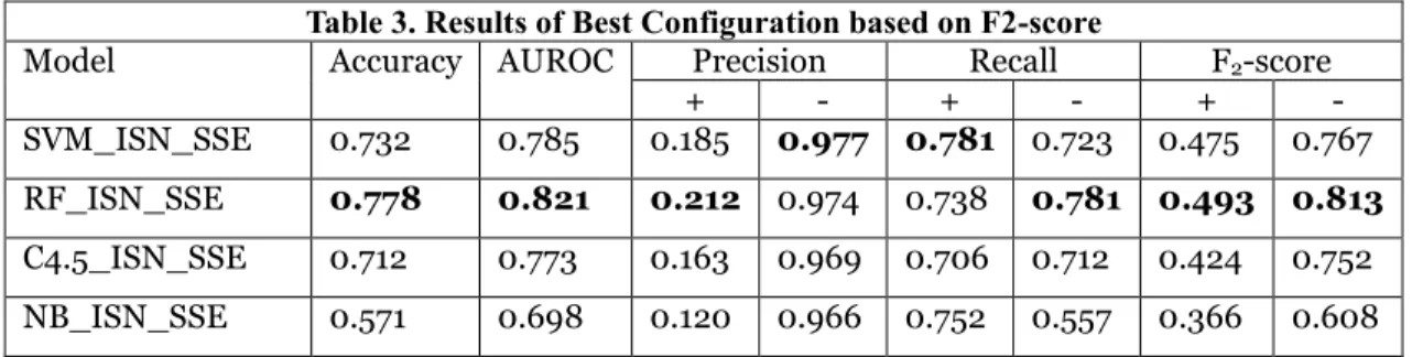
Given the settings in the previous section, comprehensive experimental results are described for 4 algorithms with 9 configurations on the 4 evaluation metrics over two classes. The results are shown in Table 3 where Random Forest is the best among all the four not only on the F2-score, but also on all the
other metrics except negative precision and positive recall. The results also indicate Naïve Bayesian is not as competitive as the other three. Among the four, SVM provides the best positive recall of 78.1% with 18.5% positive precision but Random Forest is more balanced with a positive recall of 73.8% and a positive precision of 21.2%. Their performance on the negative class are much better with over 97% precision and 70% recall rate so that their overall accuracy is over 73%. This indicates that our models are not over-fitting aggressively to predict positive samples.
Regarding the contribution of our new features, all the algorithms perform better with the extended feature set. Three algorithms (SVM, Random Forest, and C4.5) perform best with a full feature group of ISD, network features and spatial sequences features while Naïve Bayesian performs best with ISD plus network features. The result of the best data balancing technique configuration is consistent: all four gain the best performance using the SplitBal with Stacking Ensemble solution.
Table 3. Results of Best Configuration based on F2-score
Model Accuracy AUROC Precision Recall F2-score
+ - + - + -
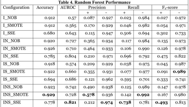
SVM_ISN_SSE 0.732 0.785 0.185 0.977 0.781 0.723 0.475 0.767 RF_ISN_SSE 0.778 0.821 0.212 0.974 0.738 0.781 0.493 0.813 C4.5_ISN_SSE 0.712 0.773 0.163 0.969 0.706 0.712 0.424 0.752 NB_ISN_SSE 0.571 0.698 0.120 0.966 0.752 0.557 0.366 0.608 We demonstrate the effectiveness of our new feature and data balancing techniques by examining the results of all configurations of Random Forest. As illustrated in Table 4, without data balancing, the positive recall is extremely low (2.3% for I_NOB), which confirms that the minority class will be ignored without proper balancing technique. In particular, SSE is more effective than SMOTE in increasing minority recall rate. If we fix the data balancing configuration, and compare performance between feature groups, our network features provide obvious performance improvements for the positive class. For instance, if we compare I_NOB with IN_NOB, F2-score is increased from 0.o27 to 0.135. Similarly, F2-score is increased
from 0.302 to 0.475 if we compare I_SSE with IN_SSE. The improvements from spatial sequences features are less significant than with network features. Under the best balancing settings, F2-score is increased from
0.302 to 0.333 if we compare I_SSE with IS_SSE. Similar gains are observed for the positive group. Recall and AUROC performance increases slightly if we add only spatial sequence features. Using all three feature groups, we obtain the best performance in terms of AUROC, positive recall and F2-score.
Lastly, we compare the performance between first term retention and first year retention predictions. As mentioned earlier, 6 networks (first 12 weeks of data) are used in first term retention prediction. Similarly, first year retention prediction is based on 14 networks (8 networks from Fall semester and 6 from Spring semester). In Table 5, we pick the best configuration for each task using Random Forest with a full feature group and SSE. The difference is that we added ‘Fall GPA’, ‘Spring student loan’ and ‘Sprint qualified tuition free’ to ISD. Adding these features almost double the precision of positive class identification (21.2% to
40%). This confirms the power of GPA in identifying students as risk. However the positive recall rate and F2-score are slightly better in the term prediction. We can interpret the result as: drop-out students are
highly likely to have low social and campus integration. Nevertheless, a student with low social or campus integration may not necessarily drop-out. However, if we know this student also has a low academic performance, then the likelihood of dropping-out increased significantly. This finding indicates that our new features (network and spatial sequences) make the most contribution to improving recall and F2-score.
An academic performance indicator that is available before the end of first semester can potentially improve our model precision for positive class.
Table 4. Random Forest Performance
Configuration Accuracy AUROC Precision Recall F2-score
+ - + - + - I_NOB 0.912 0.57 0.087 0.927 0.023 0.984 0.027 0.972 I_SMOTE 0.912 0.565 0.170 0.929 0.046 0.982 0.054 0.971 I_SSE 0.680 0.643 0.115 0.947 0.506 0.694 0.302 0.733 IN_NOB 0.920 0.727 0.365 0.934 0.117 0.984 0.135 0.973 IN_SMOTE 0.926 0.710 0.464 0.933 0.106 0.990 0.126 0.978 IN_SSE 0.785 0.804 0.210 0.971 0.696 0.792 0.475 0.822 IS_NOB 0.918 0.574 0.209 0.929 0.038 0.975 0.045 0.987 IS_SMOTE 0.922 0.660 0.355 0.931 0.077 0.977 0.091 0.989 IS_SSE 0.694 0.686 0.121 0.962 0.595 0.701 0.333 0.741 INS_NOB 0.923 0.742 0.490 0.938 0.125 0.989 0.147 0.978 INS_SMOTE 0.929 0.728 0.578 0.936 0.142 0.992 0.167 0.980 INS_SSE 0.778 0.821 0.212 0.974 0.738 0.781 0.493 0.813
Table 5. Term vs. Year Prediction
Task Accuracy AUROC Precision Recall F2-score
+ - + - + -
Term 0.778 0.821 0.212 0.974 0.738 0.781 0.493 0.813 Year 0.72 0.773 0.4 0.909 0.721 0.72 0.622 0.751
Conclusion and Future Work
In this paper, we present a novel big data approach to predict student retention. Prior work focused on a behavioral approach to gauge student integration or used data-driven learning techniques on readily available ISDs. Both approaches have their advantages and limitations. In our approach, we leverage the availability of ISDs and supplement it with student integration features to facilitate higher quality and timely predictions. The most novel aspect of our model is that it uses smart card transactions to extract implicit interactions and spatial sequences on which we apply network analysis and sequence learning methods to extract features to infer students’ social and campus integration. We design network metrics to measure students’ campus social integration using implicit networks and examine the evolution of these networks over time. Through modeling students’ daily routine as spatial sequences, we are able to capture the regularity of their activity levels and use it to infer how well they are integrated into the university environment. These features fill gaps in previous research that solely consider ISDs to predict student retention. Our evaluations show that the new features are effective in significantly improving precision and
Thirty Sixth International Conference on Information Systems, Fort Worth 2015 15 recall rates in identifying drop-out students. We also address the imbalanced-class learning issues for student retention prediction where the students at-risk are the minority class. Our experiments which compare multiple techniques with and without balancing demonstrate the necessity of data balancing. The balancing technique we applied in this study can be a competitive choice for researchers to consider. Furthermore, our approach enables us to make proactive predictions before knowing a student’s first term GPA. Most of the previous studies consider the freshmen retention problem as seen at the end of the first year, but our method provides its unique value in practice by identifying at-risk students early. This allows the university administration to identify at-risk students and implement interventions within the first semester itself.
The experimental results confirm the importance of social and campus integration in student retention. Given the high recall rate of our proactive prediction, it provides actionable decision support for university administration to perform student interventions. The limitations of our current work is that in our efforts to improve the recall rate (i.e., minimize missing at-risk students) a trade-off was made that identifies some students at risk of dropping out (who in fact did not drop out). This may increase the cost of interventions (as the target population is larger). Potential future work directions are: 1) Test and validate our prediction model on multiple years of student data; 2) Refine the imbalanced classification algorithm. So far, we have not looked deep into the classification algorithms and corresponding data balancing techniques to specifically modify them for the student retention problem. Dedicated research on this topic will be helpful to improve prediction performances. 3) Include additional academic and student integration data into the model, e.g., currently we do not have within-semester student performance for courses they are enrolled in during the first semester (e.g., on assignments or mid-semester tests) as these are not typically available in an ISD. Further, the network analysis and sequence learning methods we used to extract features from smart card usage can also be used with other kinds of data involving students’ interactions and spatial information. Potential resources from which student data can be gleaned include course management systems, campus recreation facility utilization, and Wi-Fi and LAN usage data. Together, these can supply additional academic features and allow us to create networks with different semantics which provide more comprehensive aspects about students’ campus life.
References
Astin, A. W. 1999. “Student Involvement: A Developmental Theory for Higher Education,” Journal of College Student Development (40:5), pp. 518–529.
Bean, J. P. 1982. “Conceptual Models of Student Attrition: How Theory Can Help the Institutional Researcher,” New directions for institutional research (1982:36), pp. 17–33.
Blondel, V. D., Guillaume, J.-L., Lambiotte, R., and Lefebvre, E. 2008. “Fast Unfolding of Communities in Large Networks,” Journal of Statistical Mechanics: Theory and Experiment (2008:10), p. 10008. Cabrera, A. F., Nora, A., and Castaneda, M. B. 1993. “College Persistence: Structural Equations Modeling
Test of an Integrated Model of Student Retention,” Journal of Higher Education (64:2), pp. 123–139. Caison, A. L. 2007. “Analysis of Institutionally Specific Retention Research: A Comparison between Survey
and Institutional Database Methods,” Research in Higher Education (48:4), pp. 435–451.
Delen, D. 2011. “Predicting Student Attrition with Data Mining Methods,” Journal of College Student Retention: Research, Theory and Practice (13:1), pp. 17–35.
He, H., and Garcia, E. a. 2009. “Learning from Imbalanced Data,” IEEE Transactions on Knowledge and Data Engineering (21:9), pp. 1263–1284.
Herzog, S. 2005. “Measuring Determinants of Student Return VS. Dropout/Stopout VS. Transfer: A First-to-Second Year Analysis of New Freshmen,” Research in Higher Education (46:8), pp. 883–928. Hoffman, M., Richmond, J., Morrow, J., and Salomone, K. 2002. “Investigating ‘Sense of Belonging’ in
First-Year College Students,” Journal of College Student Retention (4:3), pp. 227–256.
Lauría, E. J. M., Baron, J. D., Devireddy, M., Sundararaju, V., and Jayaprakash, S. M. 2012. “Mining Academic Data to Improve College Student Retention: An Open Source Perspective,” Proceedings of the Second International Conference on Learning Analytics And Knowledge - LAK ’12, May, pp. 139– 142.
Lin, S. 2012. “Data Mining for Student Retention Management,” Journal of Computing Sciences in Colleges (27:4), pp. 92–99.
Nandeshwar, A., Menzies, T., and Nelson, A. 2011. “Learning Patterns of University Student Retention,” Expert Systems with Applications (38:12), Elsevier Ltd, pp. 14984–14996.
Ratcliff, J. W., Metzener, D. E. 1988. "Pattern Matching the Gestalt Approach." Dr. Dobbs Journal (13:7), pp. 46.
Reason, R. D. 2009. “Student Variables that Predict Retention: Recent Research and New Developments,” Journal of Student Affairs Research and Practice, pp. 126–136.
Sarker, F., Tiropanis, T., and Davis, H. C. 2014. “Linked Data, Data Mining and External Open Data for Better Prediction of at-risk Students,” 2014 International Conference on Control, Decision and Information Technologies (CoDIT), IEEE, pp. 652–657.
Schneider, M. 2010. “Finishing the First Lap: The Cost of First Year Student Attrition in America’s Four Year Colleges and Universities,” American Institutes for Research, p. 23.
Scott, M., Spielmans, G. I., Julka, D. C., and Of, P. 2004. “Predictors of Academic Achievement and Retention Among College Freshmen: a Longitudinal Study,” College Student Journal (1:38.1), pp. 66– 80.
Sparkman, L. A., Maulding, W. S., and Roberts, J. G. 2012. “Non-cognitive Predictors of Student Success in College,” College Student Journal (46:3), pp. 642–653.
Thammasiri, D., Delen, D., Meesad, P., and Kasap, N. 2014. “A Critical Assessment of Imbalanced Class Distribution Problem: The Case of Predicting Freshmen Student Attrition,” Expert Systems with Applications (41:2), Elsevier Ltd, pp. 321–330.
Tinto, V. 1975. “Dropout from Higher Education: A Theoretical Synthesis of Recent Research,” Review of Educational Research (45:1), pp. 89–125.
Tinto, V. 2006. “Research and Practice of Student Retention: What Next?” Journal of College Student Retention2 (8:1), pp. 1–19.
Sun, Z., Song, Q., Zhu, X., Sun, H., Xu, B., and Zhou, Y. 2014. “A Novel Ensemble Method for Classifying Imbalanced Data,” Pattern Recognition (48:5), Elsevier, pp. 1623–1637.
Wang, Y., and Ram, S. 2015. “Predicting Location-Based Sequential Purchasing Events by Using Spatial, Temporal, and Social Patterns,” IEEE Intelligent Systems (30:3), pp. 10–17
Yadav, S. K., and Pal, S. 2012. “Data Mining : A Prediction for Performance Improvement of Engineering Students using Classification,” World of Computer Science and Information Technology Journal WCSIT (2:2), pp. 51–56.
Zhang, Y., Oussena, S., Clark, T., and Hyensook, K. 2010. “Using Data Mining to Improve Student Retention in Higher Education: a Case Study,” Proceedings of the 12th International Conference on Enterprise Information Systems, June, pp. 190–197.