Using sentiment analysis & machine learning for security price forecasting

Using Sentiment Analysis & Machine 

Learning for Security Price Forecasting 

Thesis submitted in partial fulfilment of the requirement for the degree of 

Bachelor of Science 

In  

Computer Science 

Declaration

This is to certify that the research work titled “Using Sentiment Analysis and Machine Learning        for Security Forecasting” is submitted by Jyotirmoy Roy and Abdullah Al Raihan Nayeem to the        Department of Computer Science & Engineering, BRAC University in partial fulfillment of the        requirements for the degree of Bachelor of Science in Computer Science. We hereby declare that        this thesis is based on results obtained from our own work. The materials of work found by other        researchers and sources are properly acknowledged and mentioned by reference. This thesis,        neither in whole nor in part, has been previously submitted to any other University or Institute        for the award of any degree or diploma. We carried our research under the supervision of Dr.        Mahbub Majumdar and Moin Mostakim    Signature of Supervisor:        _​Signature of Co­Supervisor:    ______________________   ______________________  Dr. Mahbub Majumdar Moin Mostakim  Supervisor Co­Supervisor  Department of CSE Department of CSE,  BRAC University BRAC University    Signature of authors:    ______________________ ______________________  Jyotirmoy Roy, Abdullah Al Raihan Nayeem,  15141006 12101034  

BRAC University 

FINAL READING APPROVAL 

This final report on our research is read and approved by the supervisor Dr. Mahbub Majumdar.        Its format, citation and bibliographic style are consistent and acceptable. Its illustrative materials        including figures, tables and charts are in place. The final manuscript is satisfactory and is ready        for submission to the Department of Computer Science & Engineering, School of Engineering &        Computer Science, BRAC University.            Signature of Supervisor:        _​Signature of Co­Supervisor:    ______________________   ______________________  Dr. Mahbub Majumdar Moin Mostakim  Supervisor Co­Supervisor  Department of CSE Department of CSE,  BRAC University BRAC University 

Acknowledgements 

We would like to start by thanking our thesis supervisor Dr. Mahbub Majumdar for allowing us        to work on this thesis under his supervision and for his inspiration, ideas and suggestions to        improve this work. He has offered us help to understand and supported at many difficult stages        of our work.  

We would also like to thank our co­supervisor Mr. Moin Mostakim for extending every possible        help when asked for and giving his valuable time to discuss ideas and help with machine learning        concepts.  

We are also grateful to Quantopian, Sentdex and Accern for the free and extremely helpful        resources of historic security price and sentiment analysis. 

ABSTRACT 

We worked with sentiment analysis and supervised machine learning to forecast the security        movements in stock market and benefit from it. Text rich data sources like newspapers, blogs,        stock market related internet forums, social networking websites contain relevant and updated        information about the publicly listed companies. Sentiment analysis can help us to extract usable        information from these texts to understand the overall sentiment of the articles. 

In our research, we used two sentiment analyzed database provided by Accern [1] &        Sentdex [19] and tried to see how positive is the relation between the market sentiment and        market movement of S&P 100 index listed companies. We also implemented machine learning        agent trained on the price data to find a comparable result. 

With our implementation we have been able to consistently perform better than the        benchmark with low beta and sharpe which suggests that algorithms based on state­of­the­art        sentiment analyzed data can follow the market movement stably. We have also seen that        machine learning agent trained on the price data can move with the market given a higher initial        investment.           

TABLE OF CONTENTS

CHAPTER 6  6.1 Portfolio Management………  6.2 Buying Strategy………...……….  6.3 Selling Strategy………….………..  6.4 Short Position………..………    CHAPTER 7  7.1 Machine Learning Approach……….………  7.2 Supervised Learning………...………  7.3 Feature Window………..………  7.4 Support Vector Machine (SVM)...……….  7.5 Logistic Regression………...…._​…_​………..………  7.6 Combined Prediction of Multiple Classifiers.………..    CHAPTER 8  8.1 Moving Average ………….………...………….  8.2 Sentdex’s Sentiment Data………...  8.3 Accern’s Sentiment Data………    CHAPTER 9  9.1 Comparison of Different Strategies………...  9.2 Impact of Investment Size………..  9.3 Merging Sentiment with Machine Learning……….    CHAPTER 10  10.1 Conclusion………....  10.2 Future Work………....    GLOSSARY……….  REFERENCES………      37  37  37  39      40  40  42  43  45  46      48  49  50      51  53  53      56  56    58  61             

LIST OF FIGURES 

LIST OF TABLES 

LIST OF ABBREVIATION

CHAPTER 1 

1.1

Introduction 

Predicting the stock market movement has been a subject of interest since 80s. Financial        Time Series is complex to predict since as much it depends on many numeric properties as well        as unquantifiable properties like public perception that forms over time about any company for        many different reasons. Therefore, the behavior of this series is inherently noisy, non­stationary        and deterministically chaotic [6].       _​The unquantifiable data of newspaper, articles, blogs however        contains information about important events that are happening around the world, which may or        may not affect the stock market. 

Sentiment analysis is a process of finding sentiment in any kind of text media. With the        advent of internet, people all over the globe has a media to convey their thought process and        opinions. Sentiment analysis can harvest these texts and tell us if the text is positive or negative        or neutral. While the outcome can be wrong sometimes, if the sentiment score of a topic or event        is aggregated from many articles or resources, this problem can be dealt with. 

Our research focuses on the synergy of these two concepts. By running sentiment        analysis on popular textual media, we tried to find how accurately our model could predict        market movement.  

Machine Learning helps an artificial agent to learn and predict a result without being        explicitly programmed. Using a training dataset, it can identify the patterns and tries to predict       

the next possible output. Our paper explores different machine learning approaches and how they        can help with security forecasting. 

1.2

Motivation 

Predicting stock market efficiently has been the holy grail of stock investors and        researchers. Investors want to beat the market and thus profit as much as possible. If the        investors could predict the market movement in advance, they could make money by acting on it.  Media has a big influence on people in general. If a news is highlighted by major media outlets,        it can sway public opinion. Besides, news outlets are source of information about what a        company is doing, how their products are faring in the market, new product announcements,        articles on financial reports of the companies among many other generic news. This information        helps both the informed and uninformed readers and can influence their perspective. Sentiment        analysis of these data would provide us information with how the company or its products are        doing according to the news and how the public are reacting to it. Traditional stock market        forecasting has mostly depended on analysing fundamental data of a company and are very        numeric database or value focused. They tend to avoid text rich media, as it is difficult to go        through them. The problem with numeric dataset is, they can tell us how the market is getting        affected, but not the reasoning. However, these reasoning might also be important, because if a        story saturation of an article is higher, it will reach to more audience and that way might have an        elongated effect on the market. 

Sentiment analysis on real time data feed would enable us to see, how quickly the market reacts        to a news published. High Frequency Trading (HFT) can take advantage of real time sentiment       

analysis. We aim to develop a day­to­day buy/selling strategy that takes advantage of sentiment        analysis to predict the security movement in the market and gain from it. 

1.3

Limitations of Sentiment & Daily Stock Data 

As we started our research, our first immediate hurdle was to find historic financial        market data. We could not find any minute, or daily interval based data (twice a day or thrice a        day) for free. The minute data is costly and not available in any public domain. We worked on        daily data, but as such we are losing a very important time frame to act upon the obtained        knowledge, as we are not reading from any data feed after the market opens. We close harvesting        data before the market opens, say 8am and a story breaks about a company at 2pm. We do not        have the ability to apply our buy/sell strategy since we do not have access to minute data and that        way a very important time frame is lost as informed users have already been acting on the market        accordingly and we cannot buy or sell with the new information until the next day. 

Another limitation of our research is the accuracy of sentiment analysis. Though with time the        accuracy of sentiment analysis has risen, sometimes it is hard for the analyzer to understand the        context. Consider this example sentence in the form of formatted text foresight taken from        marketwatch [16] 

“Oil settles under $37 for first time since the recession.” 

Though the expected result is an overly negative result. Stanford NLTK tool       _​rates the sentence      positive for failing to understand our perspective and the context. We believe as the sentiment        analysis tools improve and understand the perspective of the user, sentiment analysis will be        more relevant and accurate. 

1.4

Research Goal 

Stock market has been a playing field for investors and data analysts for a long time. As        much as it is challenging, it is also rewarding with its significant wealth gain. Hedge funds and        investors invest significant wealth and time to build algorithms that can perform with marginal        risk. Quantopian, our backtesting engine has also an open competition where anyone can join to        come up with an algorithm that can outperform others and has a low risk. After the financial        crisis of 2007­08, risk assessment is valued even more than ever, rather than just focusing on the        returns. 

This research has been a platform for us to learn about stock market, how it works and        learning about strategies that can further benefit the algorithm. We have also been trying to see        how accurate current sentiment analysis tools are and how do they work. Furthermore, this        research has also enabled us to test different machine learning approaches and experiment with        how they can benefit with an already established system or model. 

The main objective of our research is to find out how to predict the future market        movement using sentiment data which has analyzed news articles & popular blogs. Another        objective is to use machine learning to stabilize the algorithm and see if it can lower the risk        factors involvement. To find the answers to this question, we must start with a dataset of        sentiment analysis on popular news platforms. This needs to be mapped with security price data        to further analyze it and then develop strategies that gain more from the market. Then this        algorithm needs to be fed through the backtesting engine, which takes the strategy and simulates        it without any signal bias. All this ideas are combined in the final programming package. With        our research we hope to find answers to these questions: 

­ Do text rich documents such as news articles carry enough indications that its sentiment        can correlate with stock price of a company? 

­ How accurately can current sentiment analysis tools or datasets predict the market        sentiment? 

­ How machine learning can perform in the finance market trained on the price data?  We hope to answer these questions by building our model and analyzing backtests on        historic data.  

CHAPTER 2 

2.1

Literature Review 

Two theories are frequently discussed about security price forecasting ­ Efficient Market        Hypothesis (EMH) and Random Walk Theory. Proposed by Fama [5], EMH states that price of a        security is what all the investors has agreed upon based on the available information. If any new        information emerges, the market automatically adjusts according to the new information. This        should mean that an investor would not be able to beat the market consistently and can at most        predict with 50 percent accuracy. Random Walk Theory emerged at in the 70s, popularized by        Malkiel [3], it claims that past movement of security price or market cannot be used to predict        the movement, thus making it impossible to accurately predict financial time series. 

Significant researches however have opposed EMH and suggests that security movement        can be predict to some extent [4][14][11]. Bitcoin has been hailed as an example to counter EMH        [10] as the value of Bitcoin increases to ensure people hold them. However without any flow of        earnings, as it appreciates is against the proposal of EMH. It has been argued as experienced        traders tend to perform better than novice traders in a controlled environment, which again        contradicts EMH [13]. However, as the market gets more traders who use artificial intelligence        system which the market would become more efficient as time goes by [22]. 

Security analysis & forecasting has been a major field for researchers and many work has        been done to find how text rich data can help to point to the indicators of market movement.        Preis [23] in his research experimented with how big data can reveal important data about market       

trends. He found that if financial terms were analyzed and the changes in search volume terms        were taken into account, it can indicate a market movement early. Analyzing the performance of        98 search terms in Google Trends, developed a strategy that changes in search volume referring        to the term debt, which given the financial crisis has an obvious semantic connection. This        strategy was applied to the financial dataset between 2004 and 2011 yielding a 326% return.        Their algorithm specifically focused on how it could predict large movements correctly and        gained by a huge margin during the 2007 ­ 2008 financial crisis. In another paper, Helen [8]        discussed how Wikipedia usage patterns could indicate a market movement. She concluded that        usage data from December 2007 to April 2012 might have indicated the movement of investors.        Page view of the key terms concerning the companies that were about to fall increased before the        financial time series slumped.  

Falinouss [15] worked on the Iranian financial market. Using machine learning she was        able to predict market movement correctly with an accuracy of 83% and outperformed random        labelling which had an accuracy of 51%.  

Bollen, Mao & Zeng [9] worked extensively with twitter data feed. Using tweets as the        source of sentiment data source, they tried to see if there was any correlation between large scale        data and DJIA (Dow Jones Industrial Average) using text processing. They have found a strong        correlation between public mood and DJIA, but could not find the causative. 

Schumaker and Chen [17] used financial news articles as the learning method for their        model which according to the authors fared better than linear regression. Same duo also came up        with another paper[18] that used breaking financial news which gave them a return of 2.06% in a        span of 5 weeks. 

Das and Prady [21] worked on using Machine Learning classifiers to predict the Indian        stock market. In their research, they focused on two very popular techniques of supervised        learning ­ Back Propagation Technique (BP) and Support Vector Machines (SVM). According to        their findings, performance of SVM classifiers are much better compared to Backpropagation        Technique. Training a support vector machines requires a function with linear complexity which        optimizes the cost. Prediction of SVM is more precise when sample space of data is bigger than        its dimension. 

Kim [12] also showed few advantages of using Linear SVM over Neural Networks to        predict the financial time series. The result of his experiment infers that the value of upper bound        and the kernel parameter plays a sensitive role in performance of SVM’s prediction. The best        prediction performance of SVM according to this study is 64.75% which beats BP and Case        Based Reasoning (CBR) with the value of 58.52% and 51.98% accordingly. 

2.2

Methodological Biases: 

Since a lot of training procedure is about feeding past data as a future emulation for the   algorithm, there is higher chances to be biased to the data and noise. 

a. Data Bias: The signal data that are being used to emulate could have been hard to        obtain during the actual time. These might make it data biased and not effective for real time        usage. Supposedly we can get documents that was originally published in 03:30 PM on January        29, 2009. However, that data wasn’t available till 7:30 PM. Such issues would cloud the ability        to evaluate in real time. 

b. Signal Bias: Since we are already aware of what particular events in the past had a        major impact on the stock market, the algorithm could have been tweaked to reflect that. It’s        relatively easy to make an algorithm pick up particular shares at the right time to make a huge        profit, which might perceive the algorithm being successful.  

c. Data Noise: Sometimes a keyword (suppose name of company) can be mentioned in an        article that is not totally relevant. However, that might change value of different variables related        to that company. This type of noise would be very hard to avoid. One approach to overcome this        problem is to source the data from many different sources and compare the signal stability        between variable value changes from different sources before actually changing the value in the        database.     

CHAPTER 3 

3.1

Sentiment Analysis 

Sentiment analysis has several approaches and often a model is based on combination of  many layer of techniques to reach the conclusion. 

In bag­of­words approach a text is broken down to words, or a string of words and it does        not focus on the context in the sense that this model incorporates a large dictionary of words that        carry different level of sentiment. The words in the dictionary are then matched with the words        and value of sentiment in the words are found. All the values are added up to reach the final        sentiment valuation. There are different equations which helps with the addition and derivation        of sentiment value, but it does not focus on the fundamental aspect of a language ­ understanding        it. Bag­of­Words approach needs machine learning to produce a decent result. With a machine        learning, finding a pattern is the goal through the weighted sentiment values of the words. 

Another approach, Natural Language Processing tries to understand the text. This        approach focuses on getting the structure of the sentence, tries to learn the grammar and finds out        about the context. Parts of Speech (POS) tagging is used to determine which word of the        sentence belongs to which parts of speech. Named Entity Recognition helps to find the named        entities. This is how we can find out about the topic or matter of discussion in the topic. 

Now after chunking the text into groups of phrases like, noun and adjective & adverbs we        can find out the information about that particular named entity. From this a positive or negative        sentiment score can be derived for that named entity. 

3.2

Web Indexing 

Sentiment analysis depends on text mining. Data is to be mined from sources that are        relevant to the companies. Initially our target was to track XLK (Technology Select Sector        SPDR fund)   _​related companies, as this particular ETF tracks the technology industry which has a        massive set of news magazines, blogs, news sections specifically following them. 

To do the text mining we used Scrapy, a python framework that helps with text extraction from        websites. We targeted Techcrunch, MarketWatch etc among many other sites. To get the targeted        text, first the xpath of article header or subject and the main content has to be found. After        getting the xpath, we feed the xpath to the spider or crawler of Scrapy. Then the output is passed        to the database where it is saved for further processing. 

3.3

Language Processing Toolkit 

Natural Language Toolkit (NLTK) is a popular python library that can incorporates many        text processing features such as classification, tokenization, stemming, tagging, parsing and        semantic reasoning. We used NLTK to classify and tokenize our sample input. 

Then on our sample data, we ran the Deep Learning for Sentiment Analysis tool provided        by Stanford,_​ ​Here is an output of a sample text. 

  Figure 3.1: POS tree using Natural Language ToolKit. 

The problem with this implementation of sentiment analysis is that, it quite often fails to        understand the context. There has been multiple cases where a text carried strongly positive        sentiment, but the result we get is negative sentiment. A price increase of a company or share        gives negative result. 

We decided to use Accern[1] & Sentdex’s [19] sentiment analysis database over ours, as        they provided even more variables like event impact score, source rank which could help us        building our strategies and has been more consistent & accurate. 

3.4

Accern & Sentdex Results 

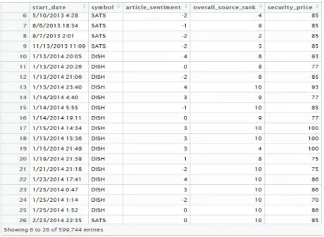
Accern ­ Actionable Trading Analysis is a company that provides a big data media        analytics and they have a public sentiment data stream for free for the time period of 2013­2014.        Accern gets its feed from 20 million data sources which are mainly news & blogs, and fetches       

about 5 million articles in a given day [1]. Accern filters out the irrelevant news sources and        claims to have 97% accuracy rate. 

Accern’s database comes with an interesting pool of variables which can be of utter        importance for coming up with a buy/selling strategy.  

Harvested at:This is a timestamp of when Accern has fetches a data source into its feed.        This can be used to map the data into the market history data       so that we don’t have the_​        information beforehand and thus avoid signal bias. 

Entity Ticker:   Ticker of the public company. This can be used to map financial data        with the company.  

First Mention:     A field with a 0 or 1 value which signifies if story is being mentioned for        the first time in the given story. 

Article Sentiment:   Accern uses a fairly complex 3 layer approach to find sentiment in an        article. In first layer they calculate the sentiment using deep learning mechanism. Then in second        layer it uses bag of words which is basically comparing the words against differently rated or        weighted positive and negative words. In the final layer n­gram is used where phrases or        particular parts of text are identified. These 3 layers give a combined linearly weighted sentiment        score within the range of ­1 to +1. 

Event Impact Score Entity:       The impact is what Accern thinks if the story has any        chance of affecting the stock price by more than 1% at the end of the trading day.  

Event Impact Score Overall:       The same is event impact score entity, but it finds the        same relationship for the event that is occurring. This can also work as filtering mechanism. An        article with higher impact score has more readership, hence can influence more people. 

Event Source Rank:     Event source rank provides information on the trustworthiness of        the news source. This can help us filtering the news articles we might want to ignore. 

Average Day Sentiment:     This provides a sentiment score within the range of ­1 to 1        based on the aggregated sentiment of the stories related to the company in a day. 

  Table 3.1: Sample data from Accern’s Sentiment Analysis. 

Sentdex is another organization that works on sentiment analysis. They pull their stories        and articles from 20 different sources like Reuters, Bloomberg, WSJ, Yahoo Finance among        many. By using “Named Entity Recognition”, it finds named entities which can tell the system        about the subject/subjects being talked about in the article. Then Sentdex applies Natural        Language Processing which involves chunking the data into many pieces which is then        compared against the adverbs, adjectives that were used to find out how the author presented the        article or named entity as ­ positively or negatively [20]. Sentdex’s sentiment score is a little        different. It’s value ranges from ­3 to +6, while ­3 would mean strongly negative sentiment, +3        means strongly positive sentiment. 0 represents neutral sentiment. Sentdex’s dataset also comes       

up with moving average of sentiment for last 100, 250, 500 and 5000 days. The timeline of the        database is Oct, 2012 to June 15, 2015. 

3.5

Pre­processing of Data 

The final dataset of both Accern and Sentdex is huge. Accern’s database has 599,744        rows and has a size of 72.16 MB, while Sentdex’s dataset has 12,242,062 rows with a total size        of 1.029 GB. Our backtest engine Quantopian does not allow to upload any csv (comma        separated value) file that takes more than 360 seconds to upload. To compress the size of our        database we removed the rows that we were not using. Even then Accern’s database could not be        uploaded. We, therefore decided to divide the Accern’s database into a chunk of companies and        worked with XLK holdings only. 

For Sentdex’s data we divided the database by the year datestamp. We had two full years of data        2013­2014 and 2014­2015 and have run our algorithm on the backtesting engine for both year        sessions. 

CHAPTER 4 

4.1

Financial Dataset 

To get the daily security price historic data, we used yahoo finance. A complex query can        fetch data for a company for the given timespan. 

http://real­chart.finance.yahoo.com/table.csv?s=YHOO&a=03&b=01&c=2013&d=01&e=28& f=2015&g=d&ignore=.csv 

The above url fetches a csv from yahoo finance, that downloads daily data stream from April 01,        2013 to February 08, 2015. By changing the company ticker, we can download historical daily        security price for any available company. 

4.2

Market Price of Stocks 

Historic price of securities are available from a few online sources, but they are always        daily based, if free. Historic price data in minutely interval is not available for free in any public        domain, which is a major setback for our system design. Since, our databases provide        information in a minute based way (for example Accern’s database has a timestamp that provides        the time of the day the article was uploaded in the Accern Data Stream), if we fail to use the        minute data we are already losing a major advantage to act upon the gained information on the        market. Currently, we stop feeding data to the system before market opens about any given date.        Even if we have information at 12 am about a major story regarding a company which might       

have significant impact on the stock price, we cannot do anything about it until the next trading        day starts.  

Our backtesting platform Quantopian supports minute based backtesting, but it does not allow to        download its security pricing data. This handicap of not getting minute data has deprived us of        further testing our analogy, propositions and ideas in a minute based frame. 

4.3

Data Mapping 

While Accern’s database has multiple fields that can be of use, it does not contain        security price data. To address it, first we downloaded daily security price data from Yahoo        Finance. Using python, we selected each individual row’s timestamp and company ticker value,        then we queried into the downloaded price data and put the value of that particular stock of that        day into the file. Sentdex’s data already had a security price data in it. Therefore it did not need        any further data mapping. 

4.4

Backtesting Engine: Quantopian 

Quantopian is our backtesting engine. It is a website that enables its user to test their        algorithm in its system. The system provides the option to run the data in daily or minute based        frame.  

Quantopian has two important methods where most of the work is done. In the ‘initialize’        method, we declare the list of companies we are interested to have in our portfolio. It defines our        universe of the companies. Also in this method we define any variables that we might be        interested to use in the code. 

Another method ‘handle_data’ gives us access to an object ‘data’, which gives us access        to all the information of companies defined in our universe in the ‘initialize’ method. It provides        us a snapshot of the defined universe on the stated time. The time interval can be set to daily and        minutely. ‘Daily’ would mean ‘handle_data’ would be called once per day and ‘minutely’ would        mean, the ‘handle_data’ method would be called in every minute of the trading day. 

Quantopian also supports uploading a csv file which can be matched against the portfolio        data using timestamp and company ticker. With the csv we can import outside information and        feed the system according to the timestamp to avoid signal bias. 

One of the drawbacks of Quantopian is that it might result in timeout error if the system        fails to fetch a csv file within 360 seconds. Since the datasets we are working with quite big, this        has been a constant hassle and major limitation to run our algorithms at its full strength. Even a        simple algorithm such as moving average takes about 4 to 5 minutes to run a backtest of 3/4        years. 

A backtest in Quantopian shows us the return over the provided time span. It also gives        us access to some very important metrics regarding the result of the implemented strategy like ­        total return, benchmark return, alpha, beta, sharpe ratio, sortino, information ratio, volatility, max        drawdown. Behavioral economics points that humans are loss averse [?]. Risk metrics can        indicate the various risk assessments that were done on the backtest and point out to the        strategies that were less risky, but achieved consistent gain. 

  Table 4.2: Risk metrics of Quantopian. 

Alpha indicates the performance return of the company compared to a benchmark, beta        indicates how much the algorithm acted against the market. Sharpe, a widely used risk        assessment indicator helps to compare an strategy to another to to find the safer risk free        approach. A sharpe ratio of more than 1 usually desirable, while a sharpe score of more than 3        would be very attractive risk adjusted return. 

Sortino ratio is similar to sharpe ratio, however it takes into account the difference        between harmful volatility and general volatility by including the standard deviation of negative        asset returns. Sortino ratio focuses more on the negative return of the portfolio than the volatility        of the approach. 

Information ratio takes into account of that fact that how consistently a strategy has        beaten the benchmark. The higher the ratio, the more is the consistency which is desirable.  

CHAPTER 5 

5.1

Attribute Dependency 

Before moving to set up the buying and selling strategy, we looked for the statistical        relations between the market price and different attributes that can possibly play a vital role for        security forecasting. Sentiment value of a specific ticker against the market value of its unit        security in a day was the main focus point. Market price's dependency on the outgoing moving        average also broaden the depth of our analysis. As a result, an initial assumption about the        impact of the these attributes was drawn to build up the further market strategy. To calculate the        dependency between the attributes, we followed two of the most conventional manners –        Pearson’s Correlation Coefficient and Linear Regression.    

5.2

Pearson’s Correlation Coefficient 

-1 ≤ _​r_​ ≤ 1

A value of ­1 indicates the negative relation between two variables which means if the value of        one variable increases then the value of other one has a tendency to decrease. On the other hand,        +1 value of      _​r _​points to the positive relation between two variables which refers that if the value       

of one variable increase, it draws same effect to the other one. However, a value of zero exhibits        no relation between the given variables. According to Pearson’s model, the formula to compute        the correlation between two variables is dividing the covariance of those variables by their        standard deviations. For instance, if the variables are       x_​ and_​  y_​ along with_​    n_​ number of rows, then_​         the correlation _​r_​ between _​x _​and _​y_​ is going to be, 

To begin with, the central idea was to observe the impact of article sentiment of a specific        ticker to operate its security price. As a continuation, after mapping the market price against the        each day’s sentiment value, we examined the correlation between these two attributes of data.        The generated result is understandably not satisfactory at all. 

Pearson’s product-moment correlation data: tmp$article_sentiment and tmp$security_price t = 45.816, df = 599640, p-value < 2.2e-16

alternative hypothesis: true correlation is not equal to 0 95 percent confidence interval:

0.05654010 0.06158456 sample estimates:

cor 0.05906271

The output of Pearson’s Correlation with the size of data frame 599,640 is denoted here        by _​cor _​which values precisely 0.05906271. A result tends to absolute zero is inferring that the        points are plotted with a wide variation instead of following the best fit line. To be specific,        Pearson’s model estimates numerically unstable correlation with large number of data as input.        Moreover, outliers in data are also one of main reasons to compromise the stability in output. For        instance, sentiment value is moving without any fraction from ­3 to 6 whereas security price has       

no fixed upper or lower bound. As a consequence, there is an abnormal distance in values of this        two attributes. In addition, the value of article sentiment is rounded to an absolute value which        also causes truncation error. In case of smaller volume of data, it would not have a huge effect on        the output but in this case, we are working on a large sample space which has a length nearly        three years with every day update. 

Furthermore, to calculate the correlation under a comparatively stable system we decided        to select the moving average of both sentiment analysis and security price of last 100 days. In        this approach, there is a fractional sentiment value available for each security price of an event.        Though, large outlier in data is still available but the truncation error is well handled through this        process. As a result, large input dataset will cause effectively less harm than before. The        following outcome of correlation is precisely 0.4056169 which is comparatively acceptable. 

Pearson’s product-moment correlation data: tmp$value_MA100 and tmp$close_MA100 t = 239.63, df = 291590, p-value < 2.2e-16

alternative hypothesis: true correlation is not equal to 0 95 percent confidence interval:

0.4025799 0.4086448

sample estimates: cor

0.4056169  

Another initial assumption about the fluctuation of ongoing market price of securities was        the impact of outgoing moving average on it. To get a more appropriate understanding, a        correlation matrix has been formed where sentiment value has been plotted against the moving        average of price which was preset in different time length. For this purpose, moving average of        last 100, 250, 500, 5000 days have been taken accordingly to observe the relation in between. 

The impact of sentiment value over the moving average of price does not seem much        stronger as we expected but the moving average certainly has a good grasp on the current market        price. At this point, the results of correlation indicate that the sentiment value cannot entirely        follow the movement of the current market but along with moving average of security prices, it        can surely be considerable to upgrade the trading strategies. 

5.3

Linear Regression Analysis 

Linear regression is another statistical convention to identify the linear relation between        two variables. Firstly, one variable is considered as explanatory or independent variable and the        other one is considered as dependent variable. For example, let       X_​ be the independent variable or_​          cause of an event and       _​ybe the dependent variable of the effect of an event. To find the regression        line, the equation would be,         y = a + bX._​         In addition, the plotted points in the graph give a best fit_​        line which represents the strength of the relation between       X_​ and_​  y_​ where_​  a_​ is the intercept and_​       b_​ 

is the slope of that line. Both the variables _​X _​and _​y _​can be explained as, 

The best fit line is determined by using the least square regression line (LSRL) which is a        method to predict a certain event following the regression model without any other given        parameters. A scatterplot of the event data provides the opportunity for better observation of        regression analysis. In this case, as we are concerned about the impact of article sentiment on the        price of the security, those value can be plotted in the graph for a better understanding. From the        huge scale of data, we have taken a partial amount to operate regression analysis and compute        the residuals to plot them against sentiment value in another graph. Scatterplot of sentiment        value against the every day opening price of the security gives a visually more efficient output of        the relation between them. 

  Figure 5.1: Scatterplot to find the statistical regression line. 

Moreover, regression analysis has few other properties such as coefficient of        determination, standard error and residual value that also help to determine the dependency of        given parameters. For the starters, coefficient of determination is basically the correlation        coefficient that we have analyzed before. Then, standard error of the regression line is the        fluctuation between the actual value of dependent variable and the predicted value according to        the analysis. In regression analysis, residual is the numerical difference between the value of        dependent variable and the upcoming predicted value. For each day, along with the sentiment        value and market price of the security, there is one residual available of the data point. Residual       

CHAPTER 6 

6.1

Portfolio Management 

We are using S&P 100 companies as our selected companies for the portfolio. Some of        the listed companies are Apple, McDonald's, Facebook, Gamestop, MSI, Caterpillar, Luluemon,        Nvidia, Lockheed Martin etc. The sector of the selected company ranges from Information        Technology, Industrial companies to Health Care.  

In the portfolio, we keep track of the current available cash. We also declare the default        investment size. In an list, we keep track of the securities we are shorting, so that we can always        keep track of those companies. After each buy or sell, the cash gets updated to the new value. 

The initial capital is set to 1M USD.   

6.2

Buying Strategy 

When moving average of price is incorporated into the algorithm, we buy when the        moving average of last fixed number of days is bigger compared to moving average of larger        value of days. For strategies that involve sentiment score, we went in for the buy when the        sentiment score is +6 (for Sentdex database, range of sentiment score: ­3 to +6) and +0.25 (for        Accern, the sentiment score is in between (­1 to +1). Sentdex’s data also comes up with the        moving average of sentiments for 100 and 300 days.  

           For Accern’s database, we bought stocks of the company if the sentiment score was        above 0.25 with a source rank more than 8 and impact score of 90. Our results are in line with        the findings of Accern [1] who used similar condition to produce a result. 

if data[stock]['article_sentiment'] > 0.25 and

data[stock]['event_impact_score_entity_1'] > 90 and data[stock]['overall_source_rank'] > 8 :

# consider to buy some position of this security

Another approach went for an aggressive buy if the story was first mentioned in the article.  Strategies where we had a machine learning agent giving an output of ­1 and +1 based on        the training data of sentiment score, we bought if the output was +1 and we hand no security        position of the company. 

6.3

Selling Strategy 

For strategies where only moving average is implemented, we sold if moving average of        longest period is greater than moving average of shorter period of days. For strategies involving        machine learning agent, we sold if the output was ­1 and we had any security position of the       

We also used a stop order percentage to minimize our chance of losing. A stop loss order        helped us to to limit the amount we could lose from a single security. 

For Sentdex, which has a sentiment output range [­3, +6 ], we exit our positions of the        security if the sentiment score is lower than ­1. For Accern, the sentiment score is less than or        equal to ­0.25 and overall source rank of 8 to prove the validity of the article. 

6.4

Short Position 

For sentiment analysis, when our system predicts a lower sentiment score and we have no        position in the company, we short a fixed amount of cash. Again, when the system predicts a        significantly better sentiment score we buy back the share. 

In the strategies, where machine learning is implemented, we append the stocks into        shorted stock list if machine learning agent gives a score ­1 (the output of the agent is ­1 and +1),        we have previously bought securities of the company and sentiment score is less than ­1.  

CHAPTER 7 

7.1

Machine Learning Approach 

Machine learning focuses on the constant development of the system by pattern        recognition through the informed data analysis. This process is tightly related to the        computational statistics where system does data extraction and search for the match. However,        instead of the human understanding, machine learning provides this observation to the system to        acquire an explicit perception on that case. To assist the prediction, machine learning can be        implemented using different strategies. Mainly, Machine learning is classified into three different        types – Supervised Learning, Unsupervised Learning, Reinforcement Learning. For the        upcoming prediction of price in our analysis, we used supervised learning to acquire the ongoing        market pattern. 

7.2

Supervised Learning 

Supervised Learning is one of the models of Machine Learning to predict the upcoming        outcome determined by training data. To begin with, this model gathers example data of given        specific attribute which refers to a set of real­world valuation. Precision in system’s observation        depends on the accuracy and length of the training examples. In our case, we trained the system        with security price of the ongoing last 100 days which is divided into the window size of 10 at a        time. This is the representation of feature vector or the object description. The amount of        description should not be too large to handle and it should contain enough indexes to compute       

accurate prediction. To generate the learning, there are two categories – Classification,        Regression. Among the multiple sets of classifiers we used Linear Support Vector Clustering        (Linear SVC), Nu­Support Vector Clustering (NuSVC) from Support Vector Machine (SVM)        and Logistic Regression to fit the features against label to compute the prediction out of the        system. As the system needs to have a proper perception the recent environment of the market,        we started to invest the cash from the portfolio after 100 days of training. As we observed that        the system performance is very unstable in first 100 days phase and it improves when training is        complete.    Figure 7.1: Initial performance of  the untrained system.  After losing most of the cash in first 100 days the system could not really get back to the  market to make profit but it more or less followed the market for the rest of the timeline. On the  other hand, with all the other variables set constant, if the investments are made on the market 

after initial training we can see a completely different scenario.   Figure 7.2: Start investing after the system is initially trained.  System runs with rise and fall almost similar to the market and makes profit of 51% out  of its capital. One more point to be noted, max drawdown is stunningly improved this time than  the untrained investment.   

7.3

Feature Window

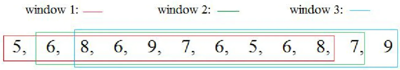
To help the system to perceive the current environment of the market, we selected the        security price of last 100 days as historical bars and set the feature window to 10. After rounding        up the differences among prices of each day in the current window we can determine if the price        is increasing or decreasing than previous window. For example, if the ongoing prices of a given        security are: 

Figure 7.3: Selecting the feature window from the security prices. 

The beginning price of every window is one shorter than the beginning price of previous window        and one more than the ending price of the last window. With the set of lists, system calculates a        feature for every window and sets the label to 1 if the ending price is greater than the beginning        price. Thus, system generates two independent sets of data – Feature & Label. For training        dataset D, 

Xi _​is the feature which has the limit from greater than or equal ­1 to less than or equal 1.        Furthermore, using different supervised learning classifiers our algorithm fits those list of        indexes to compute the prediction with the value ­1, 0 and 1. In this case, Market stability is        denoted by 0 whereas prediction 1 refers to the upcoming increment of ticker price and ­1 points        to the opposite. 

7.4

Support Vector Machines (SVM) 

Support Vector Machines (SVM) are one of the methods to perform supervised learning        using its different classifiers to predict the ups and downs of the market. In our case, in compare        to dimension of the data we have a huge amount of sample. As a consequence, the outlier       

detection should be more precise and efficient. We used python Scikit to cluster the trained data        with Linear SVC and NuSVC. 

Linear Support Vector Clustering (Linear SVC) and NuSVC are almost identical where        NuSVC is only required one more parameter to complete the calculation according to the        formula. We compared the outcomes of the investment according to both the classifiers. For        Linear SVC,  

Given the formula,         is the vector of the features of the current price list and       yi_​is the  vector of individual price label which is set by the comparison of ending price and beginning        price of the window which values ­1 and 1. 

  Figure 7.4: Total return according to the prediction of Linear SVC. 

On the other hand, NuSVC introduces a new parameter       _​which controls the support        vector and improves the training by identifying the errors in pattern. From limit 0 to 1, upper        bound of      _​indicates the training error and lower bound represents the fraction of support        vectors. As a result, max drawdown according to NuSVC is less than the Linear SVC.  

  Figure 7.5: Total return according to the prediction of NuSVC. 

However, total returns from the capital is around 5% less than the Linear SVC. In short,        in spite of the satisfactory drawdowns on both the cases, none of the total returns according to        the prediction by these classifiers can beat the benchmark returns. 

7.5

Logistic Regression 

​

To survive in the market, two of the most important decisions to make are when to

acquire and sell positions which in this case is decided the system according to the training. In        logistics regression model, the system analyses one or more independent variables to predict the       

outcome which can be either continuous or categorical and the outcome is only expressed in a        positive or negative manner. With an expression from a dependent binary variable, every time        the algorithm either goes for acquiring the position or selling the acquired position.   

  Figure 7.6: Total returns according to the prediction of Logistic regression. 

Although, the total returns according to the Logistic Regression is no improvement compared to        the Linear SVC and NuSVC but it most certainly adds a dimension to the prediction. 

7.6

Combined Prediction of Multiple Classifiers

As none of classifiers could not beat the benchmark return of the market, in spite of        achieving the market pattern, we thought of combining all the predictions together to see if the        outcomes get any better. To begin with, system gathers all predictions from the Linear SVC,        NuSVC and Logistic Regression with the same given parameters which are features and label. If        the outputs of every classifier is a common case and positive then the system goes for acquiring        the position of that specific security. In this case, prediction has results ­1, 0 and 1 given the fact        that all the other variables remain constant. One other very important parameter that we added       

that threshold the system exits that position immediately. Investing according to the new        combined prediction of the classifiers that the system used earlier, we observed that the result of        the total return gets significantly better time to time and eventually beats the benchmark.  

        Figure 7.7: Total return according to the combined prediction of the classifiers. 

Given the fact that the max drawdown decreases and alpha has now a better value that previous.        Though, total return can vary depending on the investment size and the starting portfolio cash. 

CHAPTER 8 

8.1

Moving Average 

We started off with a very simple approach, which calculates the moving average of        stock price for last 100 and 300 days. Moving average is an widely used indicator which helps        filtering price fluctuations. In this case, if we compare the moving average of 100 days and 300        days, we can see if the market is expanding or shrinking. The strategy is pretty simple ­ if        moving average of a company for last 100 days is higher, we buy stocks of that company with        10% of our total available cash. We start with 1M USD as capital, and run the backtest from        January 1, 2013 to February 28, 2014.  

  Figures 8.1: Total return using simple moving average. 

Even this simple approach gets us about 54.5% percent return with 0.90 beta and sharpe        1.57. Even though this approach initially beats the benchmark, but later fails to live up to it and        underperforms compared to the benchmark (SPY) for several months. 

8.2

Sentdex’s Sentiment Data

Then we introduced Sentdex’s sentiment data to our system. Sentdex indexes its streams        to provide a sentiment of score of an article about a company in the day of the availability of the        article. It’s sentiment score as we have discussed before is within the range or ­3 to +6.  

Our buying strategy is that If we find a sentiment score of a company, we check if the        sentiment is 6 (which means strongly positive sentiment) and we have no previous shares of this        company, we buy shares of this company with 10% worth of our available money. If our        sentiment for a company’s stock is less than or equal to ­1 and we have previously bought shares        of this company, we sell the shares. 

  Figure 8.2: Backtest using Sentdex’s sentiment data. 

This algorithm was really successful with a great return with very low beta score and a        strong sharpe score. As the algorithm picks up good stocks with positive sentiment, it starts get       

the benefit of the shares in the long run. Drawdown of just 14.8% further confirms the legitimacy        of this approach. 

8.3

Accern’s Sentiment Data

Accern’s sentiment data comes with many information field regarding the article. We        experimented with mainly four data fields ­ article sentiment, overall source rank, impact score        on entity and first mention. Article sentiment is the sentiment of the article, source rank gives a        score on the validity of the article source, impact score gives us Accern’s output of it if they        think the article has any chance of affecting the stock price of the company. First mention gives        information if the article was first to mention a story. 

If sentiment score is above .25 and source rank more than 8 with an impact score more        than 90, we get a similar return compared to the backtest using Sentdex’s sentiment data. Our        findings are in line with similar work using Accern’s data[1].        Figure 8.3: Backtest using Accern’s sentiment analysis data.     

CHAPTER 9 

9.1

Comparison of Different Strategies 

As we have established the models of our testing scenarios, we have seen some clear        results. A combined machine learning approach trained can follow the market and beat basic        strategies like moving average by a good margin. A quick comparison between these two        approaches show that the return of machine learning is 72.23% higher comparatively. It also has        53.39% less max drawdown.      Figure 9.1: Backtest of Moving Average.   

We have used the same strategy for two different sentiment analysis data, which has        given us very similar return with good risk assessment. We can see, till March 2015 (where the        timeline ends for Accern), we have the output for both graphs and till then both performs very        similarly. Accern has been consistently better from the start, but as Sentdex peaks up the pace        around, May of 2014, it has steadily performed ever since. Sharpe for both of them is more than        2.3 and Accern’s one hovers around 3 which is really good. Using Accern’s database however        has resulted in a far better sortino score & beta. It also has overperformed compared to the        benchmark (SPY) from the beginning. 

9.2

Impact of Investment Size 

We found that a change of investment size can result in a significant change in return.        When testing the result of the combined strategy, we saw that our algorithm found the pattern of        the and could follow the market movement. However, it was still underperforming, because it        wasn’t buying enough. 

Figure 9.5: Total returns in respect of investment size. 

Upon changing the investment size to a bigger one, we quickly beat the market and could stay on        top of it and follow the market. 

9.3

Merging Sentiment with Machine Learning 

In our research we have experimented with various approaches to predict the market and        tried to follow it. While some of the approaches has been more successful than the other, the        reasoning of the output told us where we could focus to improve in the next iteration. Machine        learning algorithms individually were not particularly successful, however a combination of        them has been able to garner a standard return that has consistently beaten the market. The        reasoning of this can be argued as that ­ financial market is volatile, which is why it can be taken       

advantage of. Different machine learning agents have been able to identify different volatility of        the market. When they were combined and we went for the most common prediction, we could        identify the volatility and ride with the market. Sentdex and Accern has been able to beat the        benchmark by 63.9% and 64.2% respectively, which suggests that both of the sentiment analyzed        dataset had similar output about the market. And as they have beaten the market by a large        margin, we can argue that sentiment data is reliable and accurate. 

In addition, we used both sentiment analysis (Sentdex) and machine learning in a system        to decide buying and selling strategies in the market. In this case, if the combined prediction of        machine learning agent and sentiment analysis score gives any positive signs about the price of        that security then the system goes for buy. On the other hand, If any of the model indicates        upcoming fall in price then the system exits the position of that security.   

  Figure 9.6: System performance using both Sentiment Analysis & Machine Learning. 

Besides, security position is left when any of the identifiers shows negative sign about the        upcoming situation which means the system does not take any risk at all. It considers all the        possible facts in our sample space before taking a decision. As a result, in spite of having an        impressive drawdown percentage, we did not find this approach much profitable in comparison        to single identifier approach.